Solution techniques for the vorticity-streamfunction formulation of two-dimensional ... ·...

INTERNATIONAL JOURNAL FOR NUMERICAL METHODS IN FLUIDS, VOL. 11, 515-539 (1990)

SOLUTION TECHNIQUES FOR THE VORTICITY-STREAMFUNCTION FORMULATION

OF TWO-DIMENSIONAL UNSTEADY INCOMPRESSIBLE FLOWS

T. E. TEZDUYAR, J. LIOU, D. K. GANJOO AND M. BEHR Department of Aerospace Engineering and Mechanics, and Minnesota Supercomputer Institute, Uniuersity of Minnesota,

Minneapolis, M N 55455 U.S.A.

SUMMARY A review of our solution techniques for the vorticity-streamfunction formulation of two-dimensional incompressible flows is presented. While both the viscous and inviscid cases are considered, the derivation of the proper finite element formulations for multiply connected domains is emphasized. In all formulations associated with the vorticity transport equation, the streamline upwind/Petrov-Galerkin method is used. The adaptive implicit-explicit and grouped element-by-element solution strategies are employed to maximize the computational efficiency. The solutions obtained in all test cases compare well with solutions from previously published investigations. The convergence and benchmark studies performed in this paper show that the solution techniques presented are accurate, reliable and efficient.

KEY WORDS Vorticity-streamfunction Unsteady incompressible flows

1. INTRODUCTION

In this paper we present a review of our solution techniques for the vorticity-streamfunction formulation of two-dimensional incompressible flows. We consider both the viscous and inviscid cases.

The advantages in using the vorticity-streamfunction formulation for two-dimensional computations are well known. The difficulties in this formulation are associated with the convection term in the vorticity transport equation, lack of boundary condition for the vorticity at no-slip boundaries, and determination of the value of the streamfunction at the internal boundaries for multiply connected domains.

For viscous flow problems, at no-slip boundaries corresponding to solid surfaces the variational equations needed to determine the value of the vorticity at such boundaries can be derived from the Poisson equation for the streamfunction.' This subject was also addressed in References 2-5. In problems involving multiply connected domains, an additional variational equation is needed for each internal boundary to determine the value of the streamfunction at that boundary. These additional equations can be derived by integrating the equation of motion in the velocity-pressue formulation along each internal boundary and combining the result with the variational formulation of the vorticity transport equation.' Formulations of this type can also be found, for steady problems, in References 6-8.

For inviscid flows there is no need for boundary conditions for the vorticity at solid surfaces. However, in the case of multiply connected domains the value of the streamfunction at the internal

0271-2O91/90/1305 15-25$12.50 0 1989 by John Wiley & Sons, Ltd.

Received 6 February 1989 Revised 14 April 1989

516 T. E. TEZDUYAR ET AL.

boundaries must still be determined as part of the overall solution. The additional equations needed can, again, be derived by integrating the equation of motion in the velocity-pressure formulation along each internal boundary and combining the result with the variational formulation of the Poisson equation for the streamfunction.’ Of course, whether the flow is viscous or inviscid, these difficulties related to solid boundaries do not exist for computations based on velocity-pressure formulations.10.

In all finite element formulations corresponding to the vorticity transport equation we employ the streamline upwind/Petrov-Galerkin (SUPG) method. The vorticity transport equation involves convection terms which become dominant as the Reynolds number increases. It is well known that, owing to such dominant convection terms, especially in the presence of sharp layers in the solution, regular (Bubnov-) Galerkin finite element and classical centred finite difference methods lead to spurious oscillations in the solution. The SUPG scheme minimizes such oscillations, yet introduces minimal numerical diffusion. Schemes of this type have been successfully applied to various fluid dynamics and convection-diffusion-reaction problems. ’ *, ’

In the formulations described above, implicit time integration of the spatially discretized vorticity transport equation and spatial discretization of the Poisson equation for the streamfunction lead to linear equation systems with large global matrices. For most problems of practical interest, management of these large matrices places a heavy demand on the CPU time and memory resources of the computational environment. Sometimes this demand can become too heavy even for the largest and fastest computers of our time. The two alternative solution strategies reviewed in this paper are the adaptive implicit+xplicit (AIE) solution scheme and the grouped element-by-element (GEBE) iteration method.

The implicit+xplicit algorithm proposed by Hughes and Liu14 for solid mechanics and heat transfer problems involves static allocation of the implicit and explicit elements based on stability and accuracy considerations. In Tezduyar and Liou’ the same static approach was applied to fluid mechanics problems and the AIE scheme was presented in its preliminary stage.

The AIE method is based on dynamic grouping of the elements into the implicit and explicit subsets as dictated by the element level stability and accuracy considerations. For this purpose the algorithm continuously monitors, for all elements, the Courant number and the level of variations in the solution. In this approach we can have implicit elements only where they are needed; elsewhere in the domain computations can be performed explicitly, and this of course results in substantial reductions in the computational cost involved.

The dynamic grouping involved in the AIE scheme does not have to be based on the distinction between implicitly and explicitly treated elements. The concept can be extended to other cases in which the letters ‘I’ and ‘ E in ‘AIE refer to any two procedures; and the reason for favouring one procedure over another could be based on any factor, such as the cost efficiency, the type of spatial or temporal discretizations, the differential equations used for modelling, etc. Examples of such AIE approaches can be found in Reference 16.

The GEBE method is a variation of the element-by-element (EBE) iteration method and is based on arrangement of the elements into groups with no inter-element coupling within each group. In the EBE iteration method the preconditioning matrix is chosen to be sequential product of the element level matrices. Consequently the need for the formation, storage and factorization of large global matrices is eliminated. Element level matrices can be either stored or recomputed. In the case where the element level matrices are stored, the storage need is still only linearly proportional to the number of elements. The EBE implementations in computational fluid dynamics were first reported, in the context of compressible Euler equations, by Hughes et al.” Applications to convection-diffusion equations and incompressible flows can be seen in Tezduyar et al.’* Hughes and F e r e n c ~ ’ ~ proposed EBE schemes which are based on Crout and

2D UNSTEADY INCOMPRESSIBLE FLOWS 517

Gauss-Seidel factorizations. The EBE method was also employed in conjunction with the GMRES method” by Hughes and Shakib.’l

The GEBE method has some common ground with the operator-splitting and domain decomposition methodsz2 The GEBE preconditioner is a sequential product of the element group matrices with the condition that no two elements in the same group can be adjacent. This grouping is achieved by a simple algorithm which is applicable to arbitrary meshes.23 In this form, vectorization and parallel implementation of the EBE method become very clear. To minimize the overhead associated with synchronization in parallel computations we try to minimize the number of groups.

The governing equations and the finite element formulation are given in Sections 2 and 3. The AIE and GEBE methods are described in Sections 4 and 5. We present our numerical tests and conclusions in Sections 6 and 7.

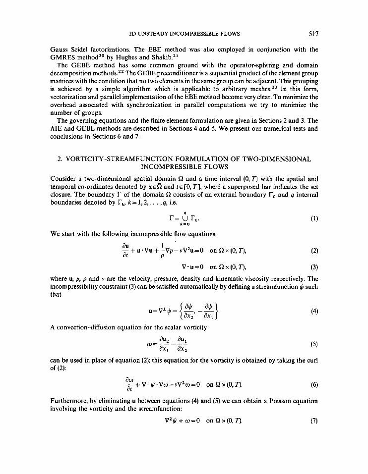
2. VORTICITY-STREAMFUNCTION FORMULATION OF TWO-DIMENSIONAL INCOMPRESSIBLE FLOWS

Consider a two-dimensional spatial domain R and a time interval (0, T ) with the spatial and temporal co-ordinates denoted by x €0 and t E [O, TI, where a superposed bar indicates the set closure. The boundary r of the domain R consists of an external boundary To and q internal boundaries denoted by rk, k = 1,2,. . . , q, i.e.

4

k = O r= u rk.

We start with the following incompressible flow equations:

au 1 - + u Vu + -Vp- vVzu=O on R x (0, T), at P

V-u=O on Rx(O,T) , (3) where u, p , p and v are the velocity, pressure, density and kinematic viscosity respectively. The incompressibility constraint (3) can be satisfied automatically by defining a streamfunction I,$ such that

A convection-diffusion equation for the scalar vorticity

w = - - L auz au ax, ax,

can be used in place of equation (2); this equation for the vorticity is obtained by taking the curl of (2):

(6) am at -++L~.Vw-vVzo=O onRx(0 ,T) .

Furthermore, by eliminating u between equations (4) and ( 5 ) we can obtain a Poisson equation involving the vorticity and the streamfunction:

518 T. E. TEZDUYAR ET AL

Remarks

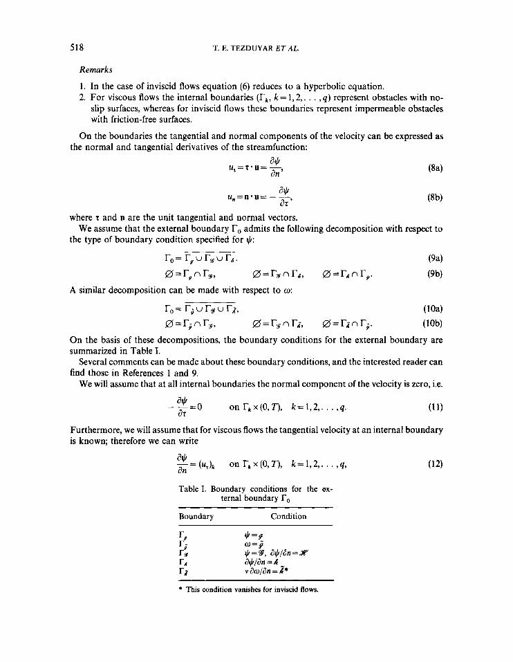
1 . In the case of inviscid flows equation (6) reduces to a hyperbolic equation. 2. For viscous flows the internal boundaries (rk, k = 1 , 2 , . . . , q ) represent obstacles with no-

slip surfaces, whereas for inviscid flows these boundaries represent impermeable obstacles with friction-free surfaces.

On the boundaries the tangential and normal components of the velocity can be expressed as the normal and tangential derivatives of the streamfunction:

where t and n are the unit tangential and normal vectors.

the type of boundary condition specified for $: We assume that the external boundary To admits the following decomposition with respect to

ro=r,ur,urR. (94 0 = r, n r,, (9b)

r,,=riurgurz, (W 0 = ri n r,, (lob)

On the basis of these decompositions, the boundary conditions for the external boundary are summarized in Table I.

Several comments can be made about these boundary conditions, and the interested reader can find those in References 1 and 9.

We will assume that at all internal boundaries the normal component of the velocity is zero, i.e.

0 = r, n r r , 0 = r, n rB. A similar decomposition can be made with respect to w:

/zr = r, n l-2, 0 = I-,- n Ti .

Furthermore, we will assume that for viscous flows the tangential velocity at an internal boundary is known; therefore we can write

Table I. Boundary conditions for the external boundary To

Boundary Condition

* This condition vanishes for inviscid flows.


where ( u ~ ) ~ is the given tangential velocity for the internal boundary k. From equation (11) we know that the value of the streamfunction is invariant along each

internal boundary; however, we do not know what that value is and therefore we need to determine it as part of the overall solution. Whether the flow is viscous or inviscid, to determine such unknown values of the streamfunction we first need to write equation (2) along each internal boundary, i.e.

au, au, 1 a p au - + + u , - + - - + v - = O on rkx(o,T), k=l ,2 , . . . , q . at 87 pi37 an (13)

lrk u,dr + :( 1.: + :)dT + v Irk Z d T = 0 on (0, T) , k = 1,2,. . . ,q. (14)

Assuming that 4.: + p/p is single-valued, the second integral on the left-hand side of equation (14) vanishes; consequently we get

From this equation we can obtain the additional equation needed to determine the unknown value of the streamfunction at an internal boundary. For viscous flows, assuming that (u,)k is invariant along r,, equation (15) leads to

where sk is the length of the boundary rk. For inuiscidflows, from (15) we get

u,dT = (constant), on (0, T), k = 1,2,. . . ,4. (17) I r k

For time-dependent problems the constants in (1 7) are evaluated from the given initial condition, whereas for steady state problems they must be given.

Finally, the initial condition for this problem consists of specification of the initial distribution of the vorticity, i.e.

o(x, 0) = wo(x) on a,. (18)

where wo(x) is a given function,

3. THE FINITE ELEMENT FORMULATION

Let 8 denote the set of all elements resulting from the finite element discretization of the computational domain Q into subdomains sz', e = 1,2,. . . ,n,,, such that

e = 1 e = l

where a,, is the number of elements. Let re denote the boundary of zz'. Let ag and Bk, k = 1,2,. . . , q, denote the set of elements adjacent to the boundaries r, and rk, k = 1,2,. . . , q, i.e.

&g={ne~ne~8, renr, # 0}, (20) &k = {ne 1 ~ ~ ~ 8 , re n r; z 01, (21) k = 1,2,. . . , 4.


We associate to 8 the following finite-dimensional space:

H ' h = { p 1 4 h E CO(Q), @I*. E P'VR"€ 8},

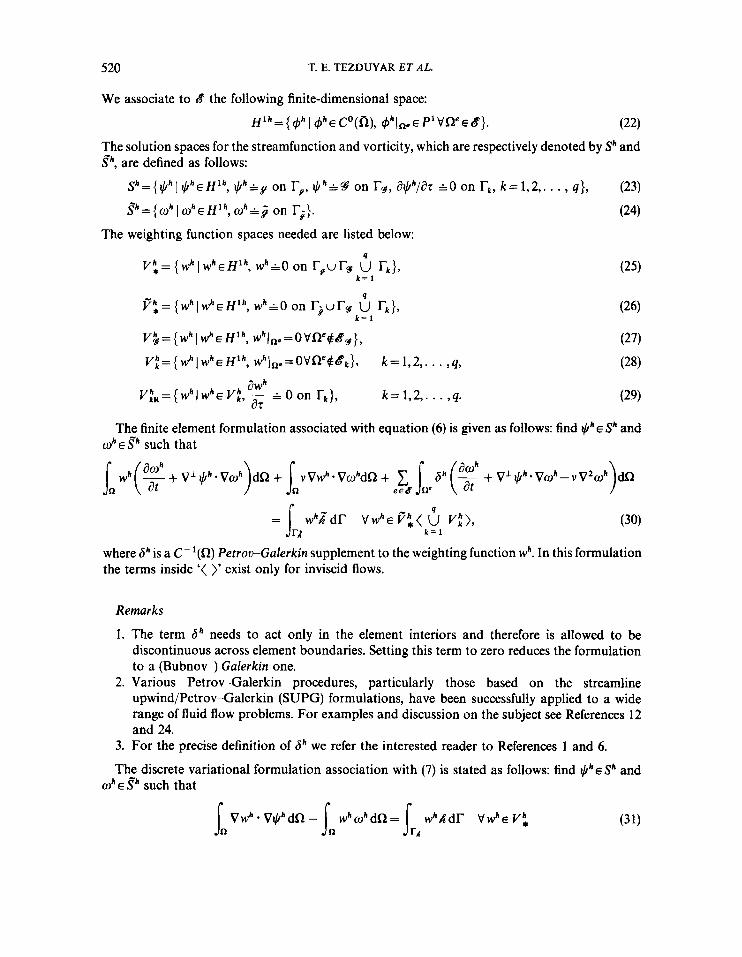
The solution spaces for the streamfunction and vorticity, which are respectively denoted by Sh and fh, are defined as follows:

~ ~ = ( * ~ ~ * ~ ~ ~ ~ ~ , l ~ l ~ = ~ o n r , , l C l ~ = ~ o n r ~ , a * ~ / a ~ e O o n r k , k = l , 2 , . . . , q} , (23)

S " h = { ~ h l ~ h ~ ~ l h , ~ h = j i on r;}. (24)

The weighting function spaces needed are listed below:

(29) awh

~ : , = { w ~ I w ~ E V : , ~ G o o n rk}, k = l , 2 , . . . ,q.

The finite element formulation associated with equation (6) is given as follows: find lLheSh and uh E fh such that

where ah is a C-'(n) Petrou-Galerkin supplement to the weighting function wh. In this formulation the terms inside '( )' exist only for inviscid flows.

Remarks

1. The term a h needs to act only in the element interiors and therefore is allowed to be discontinuous across element boundaries. Setting this term to zero reduces the formulation to a (Bubnov-) Galerkin one.

2. Various Petrov-Galerkin procedures, particularly those based on the streamline upwind/Petrov-Galerkin (SUPG) formulations, have been successfully applied to a wide range of fluid flow problems. For examples and discussion on the subject see References 12 and 24.

3. For the precise definition of ah we refer the interested reader to References 1 and 6.

The discrete variational formulation association with (7) is stated as follows: find lLh E Sh and ah E fh such that

snVwh*VtjhdQ- whAdr V W ~ E V ~ (31)


and

where the terms inside ‘< >>’ exist only for viscous flows. For viscous flows, to derive the additional variational formulations needed to determine the

values of the streamfunction at the internal boundaries, we use equation (6) and the function spaces given by (29). These variational formulations are stated as follows: find $h E Sh and mh E fh such that

- at + VL$”Bwh)dR+jR vVwh.VohdR+ e e 8 k c Jne6h($+V1$h.Voh-vVz~h)dR

Because wh is invariant along r k , the right-hand side of (33) can be obtained from (16); therefore we get

= - W h ( r k ) S k T V W ~ E V ~ R , k=l ,2 , . . . , 4 . (34)

For inviscid flows, the additional variational formulations needed are obtained by using the same function space given by (29) but in conjunction with equation (7). This leads to the following finite element formulation: find t,hh E Sh and oh E s”” such that

jR Vwh * Vl(lh dR - V W ~ E ViR, k=l ,2 , . . . , 4 . (35)

Again because wh is invariant along r k we can rewrite (35) as r r r

and by using (17) we get r r

J V W ~ * V $ ~ ~ R - J w”ohdR=wh(rk)(constant), VW~EV:!, k=l ,2 , . . . ,q. (37) n n

Now we have the complete set of equations needed to solve for all the unknowns of the problem whether the flow is viscous or inviscid. For further details of the spatial discretization and the description of the temporal discretization procedure see References 1 and 9.

The fully discretized equations can be solved in various ways. In this work we solve them either in their fully coupled form or by employing a block iteration technique. Solving them in their fully coupled form is quite straightforward and needs no explanation. The block iteration method, which is described in detail in Reference 1, requires, at every iteration, solution of mainly


two linear equation systems. These equation systems, after hiding all the subscripts and superscripts denoting the time step and iteration count, can be written as follows:

M A v = R, (38)

K d = F , (39) where the vectors v and d contain the unknown nodal values of the vorticity and streamfunction respectively. The matrices M and K are formed by assembling their element level contributors, i.e.

M = 1 Me, e ~ 8

K = 1 K'. e e 8

The right-hand-side vectors R and F, which are known at a given iteration step, are also formed by the assembly of their element level contributors.

Remarks

1. The matrix Me has the same dimensions as the global matrix M but only very few non-zero entries (e.g. 4 x 4 for a two-dimensional quadrilateral element with a scalar unknown).

2. The matrix K is symmetric and positive-definite. A particular version of the Petrov-Galerkin method employed results in M also being symmetric and positive-definite; however, we will assume that in general M is not symmetric and positive-definite.

4. THE ADAPTIVE IMPLICIT-EXPLICIT (AIE) METHOD

Let 8, and 8, be the subsets of 8 corresponding to the implicit and explicit elements, respectively, such that

b=bP, u 8,, 0 = 81 n 8,. (41)

Consequently, from equation (40a) we get

M = M'+ c M'. e e d , ' € 8 ,

(42)

The AIE schemeis based on modifying M by replacing Me( V e E gE) with its lumped mass matrix part,

M = 1 M + c Mt eeB, eeB,

(43)

The grouping given by (41) is achieved dynamically (adaptively) on the basis of stability and accuracy considerations.

The stability criterion is in terms of the element Courant number CAt which is defined as

where h is the element length.' Any element with its Courant number greater than the stability limit of the explicit method should belong to the implicit group


For the accuracy criterion we use a quantity which we expect to be a fair representative of the dimensionless wave number. O n the basis of the observations from our numerical tests we select the accuracy criterion as

0‘

(Js 0% = T, (454

where

Here 4 is a generic symbol for the dependent variable, whilef, andf, are the fluxes corresponding to directions x1 and x,. The dimensionless element level ‘jump’j‘(4) is defined as

where a is the element node number and 4: is the value of the dependent variable at node a of the element e. The instantaneous maximum and minimum values of 4 are denoted by 4,,,ax and 4min. This definition ofF(4) represents the magnitude of the variation of the solution across an element. The elements with 0% greater than a predetermined value belong to group 8,.

Borrowing from the adaptive mesh refinement technique^,,^ we also experimented with the accuracy indicator in terms of the 9,-norm of the residual r :

with

Note that all expressions are based on the ‘previous solution’. The ‘previous solution’ can come from the previous time step, non-linear iteration or pseudo-time-step iteration, whichever is appropriate.

The implementation of the AIE scheme is straightforward. A global search is performed over the entire set of elements. With this search, on the basis of the two critical parameters given by (44) and (45a) (or (46a)), the elements are grouped into the subsets 8, and 8,. Compared to having all the elements treated implicitly, this grouping results in substantial savings in CPU time and memory.

For the solution of (39) we use a preconditioned conjugate gradient method.26 In conjunction with the AIE scheme employed for equation (38), we define our preconditioning matrix P to be

P = 1 K“ + diag(K‘), e e l , e E l ,

(47)

where K‘ is the element contribution matrix of K. If gE = 0 then P= K, and the solution technique


becomes a direct one. If 8, = 0 then the method becomes a Jacobi iteration.26 Other definitions for P are of course possible; the one given by (47) is simple to implement and reflects the expectation that there may be a correlation between the solution procedures for (38) and (39).

Remarks

It is important to note that the grouping does not have to be only with respect to implicit and explicit treatments. In the acronym ‘AIE, the letter ‘I’ can refer to the ‘I-elements’ subject to some ‘I-procedure’, while the letter ‘E’ can refer to the ‘E-elements’ subject to some other ‘E-procedure’. We can employ the ‘I-procedure’ where it is neededldesired and the ‘E-procedure’ elsewhere. For further discussions and comments as well as other possible ‘I/E procedures’ see Reference 16. In the AIE approach one can have a high degree of refinement throughout the mesh and raise the implicit flag only for those elements which need to be treated implicitly. The savings in CPU time and memory can be maximized by performing, as often as desired, an equation renumbering at the implicit zones to obtain optimal bandwidths. Bandwidth optimizers are already available for finite element applications, especially in the area of structural mechanics.

5. THE GROUPED ELEMENT-BY-ELEMENT (GEBE) ITERATION METHOD

The linear equation systems (38) and (39) are both in the form

A x = b .

The iterative solution techniques used to solve (48) are described in this section.

Element grouping

The elements are arranged into ‘parallelizable’ groups in such a way that NPa

8 = u 6 K , K = 1

and such that no two elements within a group are neighbours (being neighbours is defined as having at least one common node). The number of such groups is denoted by Npg. On the basis of this grouping, the matrix A can be written as

where the ‘group matrices’ are defined as

A , = 1 A“, K = 1,2,. . . ,Npg. eeB,

Remarks

1. Because there is no inter-element coupling within each group, computations performed in element-by-element fashion (such as operations performed on a group matrix) do not depend on the ordering of the elements.


2. In parallel computations, before we can start with a new element group we first have to finish with the one that we have already started with. To minimize the overhead associated with this synchronization, we try to minimize the number of groups. A simple element grouping algorithm which serves this purpose is described in Reference 23.

3. To increase the vector efficiency of the computations performed, within each group the elements are processed in packets of ncp elements, where nep is the optimum packet size for a given vector environment (e.g. 64).

GEBE-preconditioned iterative solution method

Equation (48) is solved with a preconditioned iteration method which is built on solving

P Ay,,, =rm (52)

r,,, = b- Ax,,,. (53)

for Ay,,,, where P is the preconditioning matrix and r, is the residual vector defined as

The form of the scaling matrix W depends on the properties of A. If A is symmetric and positive- definite, one obvious choice is

W = diag A. (544 The alternative choice

W = lump M

gives a symmetric and positive-definite scaling matrix even if A is not so. Although the mass matrix comes up usually in the context of time-dependent problems, for scaling purposes it can be introduced also in the context of steady-state problems. In reality, the context in which we use this scaling matrix does not require it to be symmetric and positive-definite; it is sufficient that W is symmetric, and of course non-singular.

Two-pass GEBE preconditioner (2P-GEBE)

In this method the preconditioning matrix is defined as 1

P = fi (EKW-l) W n (W-’EK), K = l K=N, ,

(55 )

where

EK=W+$BK, K=1,2,. . . ,NPg, (56)

B,=AK-W,, K=l,2, . . . ,NPg, (574

BK=AK, K = 1,2,. . . , Npg. (57b)

with

or

The choice given by (57a) leads to ‘Winget regularization’. For comments on the relationship between the GEBE and three regular EBE methods see Reference 23.

In the next two subsections we describe the GEBE versions of the Crout- and Gauss-Seidel- factorization-based EBE preconditioners.”


Crout-factorization-based GEBE preconditioner (Crout-GEBE)

Based on the Crout factorization

W+BK=LKDKUK, K=1,2,. . . ,NPB,

the preconditioning matrix is defined as

Gauss-Seidel-factorization-based GEBE preconditioner (GS-GEBE)

Consider the following lower triangulardiagonal-upper triangular decomposition:

A , = A i + A ; + A ; , K=1,2,. . . , N , , .

Based on this decomposition the preconditioning matrix is given as

Updating the vector x,

gradient method with the preconditioners as defined in the previous subsections. If the matrix A is symmetric and positive-definite we employ a preconditioned conjugate

If the matrix A is not symmetric and positive-definite then the vector x, is updated as follows:

X m + 1 =xm+sAYm, (62)

where the search parameter s is determined by the formula

which is derived by minimizing ( 1 rm+ ( 1 ’ with respect to s.

vectorization and parallel processing of these algorithms see Reference 23. For further details and discussions on the GEBE algorithms as well as comments on the

6. NUMERICAL EXAMPLES

We have tested the fully coupled and block iterative forms of the formulation together with the AIE and GEBE methods.

Convergence and benchmark studies

Numerous researchers have performed computations for the driven cavity flow problem. We chose this problem for our convergence (based on successive mesh refinement) and benchmark (based on the CPU time and memory requirement) studies. In this test the lid of the cavity has unit velocity; based on this velocity and the dimension of the cavity the Reynolds number is 400.

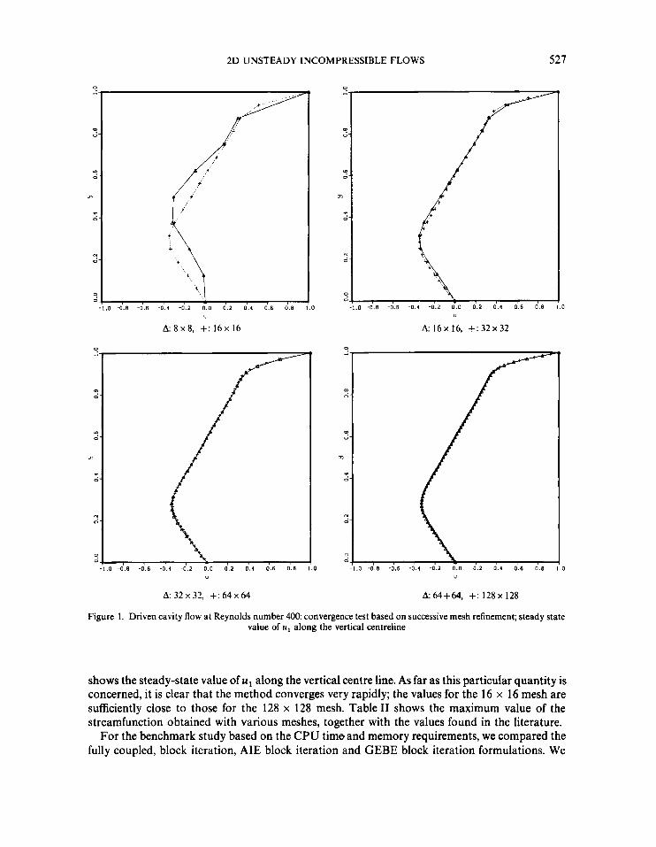
In the convergence study uniform meshes were used; the number of elements are 8 x 8,16 x 16, 32 x 32,64 x 64 and 128 x 128. We employed the GEBE solution method in conjunction with the block iteration form. The steady-state solution obtained with a given mesh was supplied (by interpolation) as the initial condition for the mesh with one level of higher refinement. Figure 1

2 D UNSTEADY INCOMPRESSIBLE FLOWS 527

3 -0.8 -0 6 -0 4 -0.2 0.0 0 2 0 4 0 6 0 8 "

A:8x8. + .16x16

A; 32 x 32, +: 64 x 64

J

0 -0.8 -0.6 -0.4 -0.2 0.0 0.2 0 . 4 0 6 0.8

A: 16 x 16. +: 32 x 32

0

m

m

n

..

N

o

0 0

-1.0 -0.8 -0.6 -0.4 -0.2 0.0 0.2 0.4 0.6 0.8 "

A: 64+64, +: 128 x 128

Figure 1. Driven cavity flow at Reynolds number 400: convergence test based on successive mesh refinement; steady state value of u, along the vertical centreline

shows the steady-state value of u1 along the vertical centre line. As far as this particular quantity is concerned, it is clear that the method converges very rapidly; the values for the 16 x 16 mesh are sufficiently close to those for the 128 x 128 mesh. Table11 shows the maximum value of the streamfunction obtained with various meshes, together with the values found in the literature.

For the benchmark study based on the CPU time and memory requirements, we compared the fully coupled, block iteration, AIE block iteration and GEBE block iteration formulations. We


Figure 2. Driven cavity flow at Reynolds number 400: solution obtained by the AIE method; vorticity, distribution of the implicit elements, and streamfunction at t=2.34, 4.69, 7.03 and 9.38


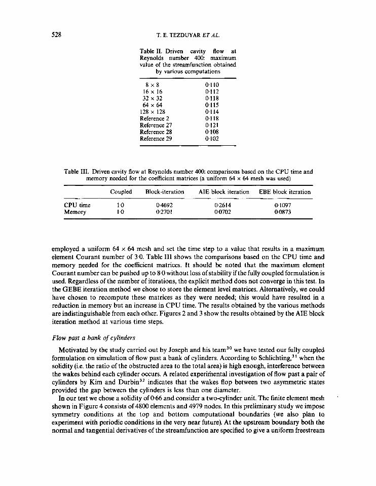
Figure 3. Driven cavity flow at Reynolds number 400: solution obtained by the AIE method; vorticity, distribution of the implicit elements, and streamfunction at t = 11.72, 14.06, 16.41 and 18.75

velocity. At the downstream boundary the normal derivative of both the vorticity and streamfunction is specified to be zero. The Reynolds number based on the freestream velocity and the cylinder diameter is 100.

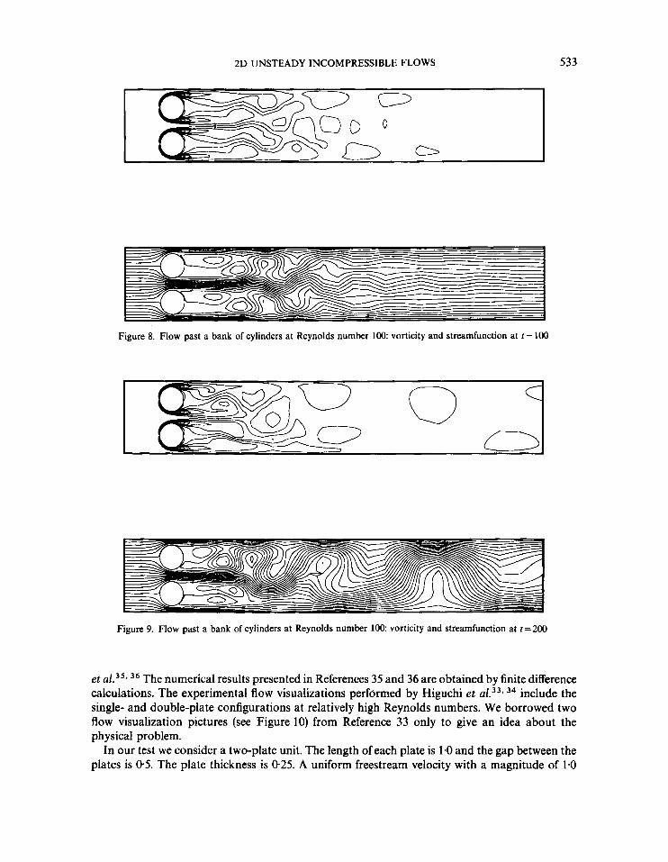
The symmetric solutions at t = 5 and t = 50 are shown in Figures 5 and 6. The steady-state solution is achieved long before t = 50. At t = 5 1, to break the symmetry an external perturbation is applied for a duration of only one time step. Figure 7 shows the solution at t=80, at which time the asymmetry becomes quite visible. The solutions at t = 100 and t=200 are shown in Figures 8 and 9.

Flow past two $at plates

Analysis of wakes behind flat plates has various applications, including the wake of a ribbon parachute and airflow through the slotted dive brakes of an aircraft.33* 34 The problem of wake interference behind two flat plates was examined experimentally and numerically by Hayashi


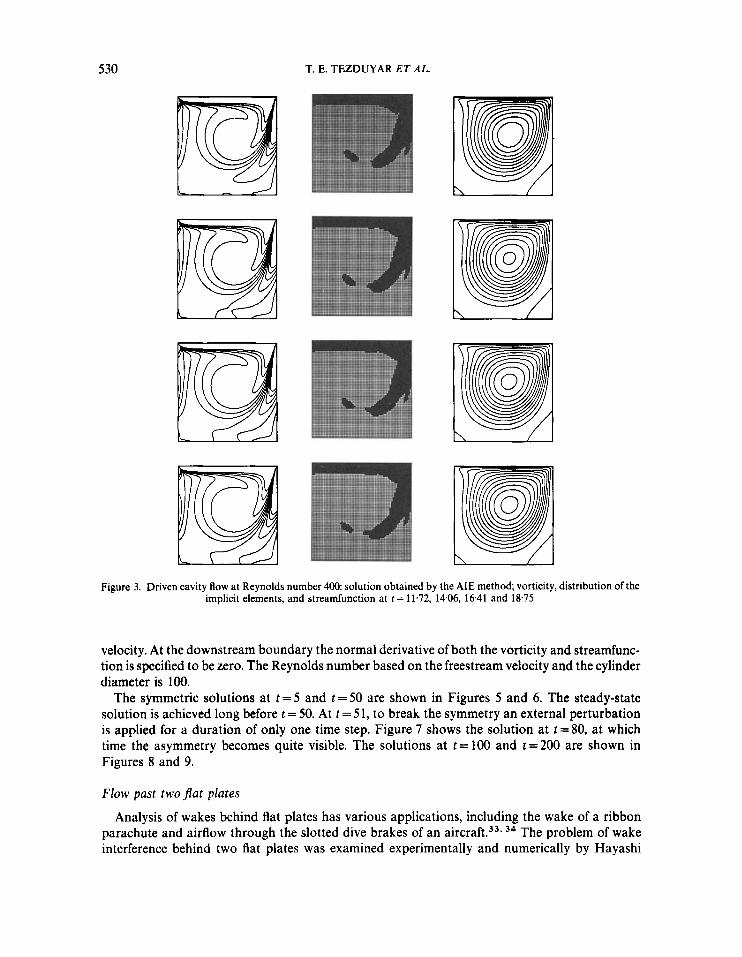
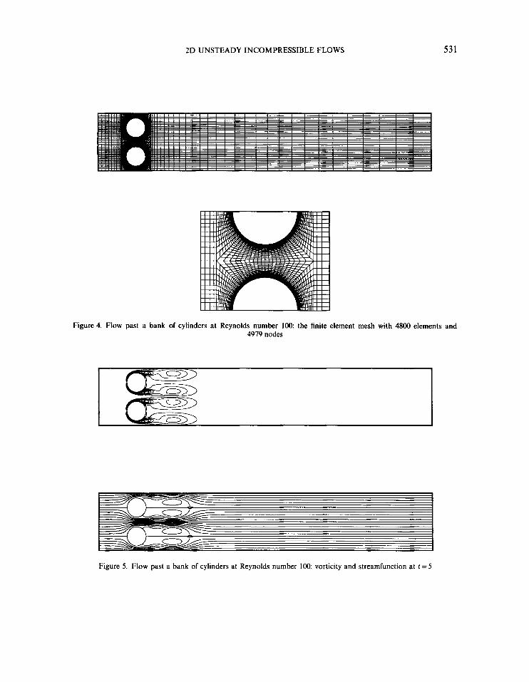
Figure 4. Flow past a bank of cylinders at Reynolds number 100: the finite element mesh with 4800 elements and 4919 nodes

Figure 5. Flow past a bank of cylinders at Reynolds number 100: vorticity and streamfunction at t = 5


I --z. I I

7

Figure 6. Flow past a bank of cylinders at Reynolds number 100: vorticity and streamfunction at t = 50

Figure 7. Flow past a bank of cylinders at Reynolds number 100: vorticity and streamfunction at t=80


Figure 8. Flow past a bank of cylinders at Reynolds number 100: vorticity and streamfunction at t= 100

Figure 9. Flow past a bank of cylinders at Reynolds number 100: vorticity and streamfunction at t=200

et ~ l . ~ ’ . 36 The numerical results presented in References 35 and 36 are obtained by finite difference calculations. The experimental flow visualizations performed by Higuchi et ~ 1 . ~ ~ . 34 include the single- and double-plate configurations at relatively high Reynolds numbers. We borrowed two flow visualization pictures (see Figure 10) from Reference 33 only to give an idea about the physical problem. In our test we consider a two-plate unit. The length of each plate is 1.0 and the gap between the

plates is 05. The plate thickness is 0.25. A uniform freestream velocity with a magnitude of 1.0


Figure 10. Flow visualizations in water for a single plate and for two plates (with gap 1.0) at Reynolds number 1400 (courtesy of H. Higuchi and H. J. Kim3’)


Figure 11. Flow past two plates at Reynolds number 50: the finite element mesh with 4374 elements and 4534 nodes

Figure 12. Flow past two plates at Reynolds number 50: vorticity and streamfunction at t = 10.0


I

Figure 13. Flow past two plates at Reynolds number 50: vorticity and streamfunction at t = 12.5

L Figure 14. Flow past two plates at Reynolds number 5 0 vorticity and streamfunction at t = 145.0


Figure 15. Flow past two plates at Reynolds number 5 0 vorticity and streamfunction at t = 1475

results in a Reynolds number of 50 based on the gap length. A non-uniform mesh consisting of 4374 elements and 4534 nodes was employed (see Figure 11).

Initially the flowfield develops symmetrically as shown in Figure 12. Transition to an asymmetric flow pattern occurs at t !z 12. Following this symmetry breaking, vortex shedding occurs (see Figures 13-1 5). These preliminary results compare well qualitatively with the results obtained by Hayashi et on an 11,528-node grid.

7. CONCLUDING REMARKS

We have presented a review of our solution techniques for the vorticity-streamfunction formulation of two-dimensional incompressible flows. We have emphasized the derivation of the proper finite element formulations for multiply connected domains. These formulations cover both the viscous and inviscid cases. In all finite element formulations corresponding to the vorticity transport equation we employed the streamline upwind/Petrov-Galerkin procedure. This procedure minimizes the spurious oscillations encountered in convection-dominated problems, yet introduces minimal numerical diffusion.

To make our computations efficient we use two solution strategies: the adaptive implicit-explicit (AIE) scheme and the grouped element-by-element (GEBE) iteration method. Such strategies become crucial for large-scale computations.

We have performed several numerical tests. In all cases the results obtained compared well with the previously published results. The convergence study (based on successive mesh refinement) for one of the test problems shows that the formulations presented are accurate and reliable. The


benchmark computations indicate that the AIE and GEBE strategies result in substantial reductions in the computational cost involved.

ACKNOWLEDGEMENTS

This research was sponsored by NASA-Johnson Space Center under contract NAS-9-17892 and by NSF under grant MSM-8796352.

REFERENCES 1. T. E. Tezduyar, R. Glowinski and J. Liou, ‘Petrov-Galerkin methods on multiply-connected domains for the

vorticity-streamfunction formulation of the incompressible Navier-Stokes equations’, Int. j . numer. methodspuids, 8,

2: A. Campion-Renson and M. J. Crochet, ‘On the stream function-vorticity finite element solutions of Navier-Stokes equations’, Int. j . numer. methods eng. 12, 1809-1818 (1978).

3. R. Glowinski and 0. Pironneau, ‘Numerical methods for the first biharmonic equation and for the two-dimensional stokes problem’, SIAM Rev. 21, 167-212 (1979).

4. M. 0. Bristeau, R. Glowinski and J. Periaux, ‘Numerical methods for the Navier-Stokes equations: applications to the simulation of compressible and incompressible viscous flows’, Computer Physics Report, Unioersity of Houston, Research Report UHIMD-4, February 1987.

5. M. F. Peeters, W. G. Habashi and E. G. Dueck, ‘Finite element stream function-vorticity solutions of the incompressible Navier-Stokes equations’, Int. j . numer. methods juids , 7 , 17-27 (1987).

6. V. Girault and P. A. Raviart, Finite Element Approximation of the Navier-Stokes Equations, Springer-Verlag, New York, 1979.

7. A. Mizukami, ‘Short communications: a stream function-vorticity finite element formulation for Navier-Stokes equations in multi-connected domain’, Int. j . numer. methods eng., 19, 1403-1420 (1983).

8. M. D. Gunzburger and R. A. Nicolaides, ‘Algorithmic and theoretical results on computation of incompressible viscous flows by finite element methods’, Comput. Fluids, 13, 361-373 (1985).

9. T. E. Tezduyar, ‘Finite element formulation for the vorticity-stream function form of the incompressible Euler equations on multiply-connected domains’, Computer Methods in Applied Mechanics and Engineering, UMSI 88/94, University of Minnesota Supercomputer Institute, October 1988.

10. P. M. Gresho and R. L. Sani, ‘On pressure boundary conditions for the incompressible Navier-Stokes equations’, R. H. Gallagher, R. Glowinski, P. M. Gresho, J. T. Oden and 0. C. Zienkiewicz (eds), Finite Elements in Fluids, Yo/ . 7, Wiley, New York, 1987, pp. 123-157.

11. P. M. Gresho and S. T. Chan, ‘Semi-consistent mass matrix techniques for solving the incompressible Navier-Stokes equations’, Lawrence Livermore National Laboratory, Preprint UCRL-99503, 1988.

12. A. N. Brooks and T. J. R. Hughes, ‘Streamline upwind/Petrov-Galerkin formulations for convection dominated flows with particular emphasis on the incompressible Navier-Stokes equations’, Comput. Methods Appl. Mech. Eng. 32,

13. T. E. Tezduyar and T. J. R. Hughes, ‘Finite element formulations for convection dominated flows with particular emphasis on the compressible Euler equations’, Proc. AIAA 2lsr Aerospace Science Meeting, Reno, NV, January 1983, AIAA Paper 834125.

14. T. J. R. Hughes and W. K. Liu. ‘Implicit-explicit finite elements in transient analysis: stability theory’, J . Appl. Mech.

15. T. E. Tezduyar and J. Liou, ‘Element-by-element and implicit-explicit finite element formulations for computational fluid dynamics, in R. Glowinski, G. H. Golub, G. A. Meurant and J. Periaux (eds), Proc. 1st Int. Symp. on Domain Decomposition Methods for Partial DifSerential Equations, SIAM, Philadelphia, PA, 1988, pp. 281-300.

16. T. E. Tezduyar and J. Liou, ‘Adaptive implicit+xplicit finite element algorithms for fluid mechanics problems’, in T. E. Tezduyar and T. J. R. Hughes (eds), Recent Developments in Computational Fluid Dynamics, AMD Vol. 95, ASME, New York, 1988, pp. 163-184.

17. T. J. R. Hughes, J. Winget, I. Levit and T. E. Tezduyar, ‘New alternating direction procedures in finite element analysis based upon EBE approximation factorizations’, in S. N. Atluri and N. Perrone (eds), Computer Methodsfor Nonlinear Solids and Mechanics, AMD Vol. 54, ASME, New York, 1983, pp. 75-110.

18. T. E. Tezduyar, J. Liou, T. Nguyen and S. Poole, ‘Adaptive implicit+xplicit and parallel element-by-element iteration schemes’, in T. F. Chan, R. Glowinski, J. Periaux and 0. B. Widlund (eds), Domain Decomposition Methods, SIAM, Philadelphia, PA, 1989, pp. 443-463.

19. T. J. R. Hughes and R. M. Ferencz, ‘Fully vectorized EBE preconditioners for nonlinear solid mechanics: applications to large-scale three-dimensional continuum, shell and contact/impact problems’, in R. Glowinski, G. H. Golub, G. A. Meurant and J. Periaux (eds), Proc. 1st Int. Symp. on Domain Decomposition Methods for Partial Differential Equations, SIAM, Philadelphia, PA, 1988, pp. 261-280.

1269-1290 (1988).

199-259 (1982).

45, 371-374 (1978).


20. Y. Saad and M. H. Schultz, GMRES: a generalized minimal residual algorithm for solving nonsymmetric linear

21. T. J. R. Hughes and F. Shakib, private communications, 1988. 22. R. Glowinski, Q. V. Dinh and J. Periaux, ‘Domain decomposition methods for nonlinear problems in fluid dynamics’,

Comput. Methods Appl. Mech. Eng. 40, 27-109 (1983). 23. T. E. Tezduyar and J. Liou, ‘Grouped element-by-element iteration schemes for incompressible flow computations’,

Computer Physics Communications, UMSI 88/95, University of Minnesota Supercomputer Institute, October 1988. 24. T. J. R. Hughes, ‘Recent progress in the development and understanding of SUPG methods with special reference to

the compressible Euler and Navier-Stokes equations’, in R. H. Gallagher, R. Glowinski, P. M. Gresho, J. T. Oden and 0. C. Zienkiewicz (eds), Finite Elements in Fluids, Vol. 7, Wiley, New York, 1987, pp. 273-287.

25. G. F. Carey and J. T. Oden, Finite Elements: Computational Aspects, Vol. 3, Prentice-Hall, Englewood Cliffs, NJ, 1984. 26. R. Glowinski, Numerical Methods for Nonlinear Variational Problems, Springer-Verlag, New York, 1984. 27. M. D. Olson and S. Y. Tuann, ‘Primitive variables versus stream function finite element solutions of the Navier-Stokes

28. S. Ozawa, ‘Numerical studies of steady flow in a two dimensional square cavity at high Reynolds numbers’, J . Phys.

29. 0. C. Burggraf, ‘Analytical and numerical studies of the structure of steady separated flows,’ J . Fluid Mech., 24,

30. P. Singh, P. Caussignac, A. Fortes, D. D. Joseph and T. Lundgren, ‘Stability of Periodic arrays of cylinders across the

31. H. Schlichting, Boundary-Layer Theory, 7th edn., McGraw-Hill, New York, 1979, pp. 744-745. 32. H. J. Kim and P. A. Durbin, ‘Investigation of the flow between a pair of circular cylinders in the flopping regime’,

J . Fluid Mech., 196, 431-448 (1988). 33. H. Higuchi and H. J. Kim, ‘Flow visualizations and mean pressure and velocity measurements behind the grid models’,

Sandia Report 48-2215, Department of Aerospace Engineering and Mechanics, University of Minnesota, April 1986. 34. H. Higuchi and F. Takahashi, ‘Flow past two-dimensional parachute models,’ J. Aircraji; also AIAA Paper 88-2524,

1988. 35. M. Hayashi, A. Sakurai and Y. Ohya, ‘Numerical and experimental studies of wake interference of two normal flat

plates at low Reynolds numbers’, Mem. Fac. Eng., Kyushu Unio., 43, 165-177 (1983). 36. M. Hayashi, A. Sakurai and Y. Ohya, ‘Wake interference of a row of normal flat plates arranged side by side’, J . Fluid

Mech., 164, 1-25 (1986).

systems’, Research Report YALEU/DCS/RR-254, 1983.

equations’, Finite Element Methods in Flow Problems, S. Margherita Ligure, 1976, pp. 5 7 4 8 .

SOC. Japan, 38, 889-895 (1975).

113-151 (1966).

stream by direct simulation of steady flow’, J . Fluid Mech., in the press.

Date post:	23-Jun-2018
Category:	Documents
Upload:	vokhuong
View:	220 times
Download:	0 times

Solution techniques for the vorticity-streamfunction formulation of two-dimensional ... ·...

Documents