Solved with COMSOL Multiphysics 5.2 1 | HEAT SINK Heat Sink Introduction This example is intended as a first introduction to simulations of fluid flow and conjugate heat transfer. It shows the following important points: • How to draw an air box around a device in order to model convective cooling in this box. • How to set a total heat flux on a boundary using automatic area computation. • How to display results in an efficient way using selections in data sets. The application is also described in detail in the book Introduction to the Heat Transfer Module. An extension of the application that takes surface-to-surface radiation into account is also available; see Heat Sink with Surface-to-Surface Radiation. Figure 1: The application set-up including channel and heat sink. Base surface Inlet Outlet
Transcript
Solved with COMSOL Multiphysics 5.2
Hea t S i n k
Introduction
This example is intended as a first introduction to simulations of fluid flow and conjugate heat transfer. It shows the following important points:
• How to draw an air box around a device in order to model convective cooling in this box.
• How to set a total heat flux on a boundary using automatic area computation.
• How to display results in an efficient way using selections in data sets.
The application is also described in detail in the book Introduction to the Heat Transfer Module. An extension of the application that takes surface-to-surface radiation into account is also available; see Heat Sink with Surface-to-Surface Radiation.
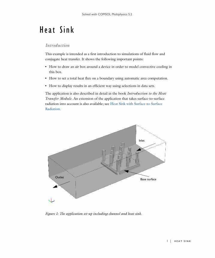
Figure 1: The application set-up including channel and heat sink.
Base surface
Inlet
Outlet
1 | H E A T S I N K
Solved with COMSOL Multiphysics 5.2
2 | H E A
Model Definition
The modeled system consists of an aluminum heat sink for cooling of components in electronic circuits mounted inside a channel of rectangular cross section (see Figure 1).
Such a set-up is used to measure the cooling capacity of heat sinks. Air enters the channel at the inlet and exits the channel at the outlet. The base surface of the heat sink receives a 1 W heat flux from an external heat source. All other external faces are thermally insulated.
The cooling capacity of the heat sink can be determined by monitoring the temperature of the base surface of the heat sink.
The model solves a thermal balance for the heat sink and the air flowing in the rectangular channel. Thermal energy is transported through conduction in the aluminum heat sink and through conduction and convection in the cooling air. The temperature field is continuous across the internal surfaces between the heat sink and the air in the channel. The temperature is set at the inlet of the channel. The base of the heat sink receives a 1 W heat flux. The transport of thermal energy at the outlet is dominated by convection.
The flow field is obtained by solving one momentum balance for each space coordinate (x, y, and z) and a mass balance. The inlet velocity is defined by a parabolic velocity profile for fully developed laminar flow. At the outlet, the normal stress is equal the outlet pressure and the tangential stress is canceled. At all solid surfaces, the velocity is set to zero in all three spatial directions.
The thermal conductivity of air, the heat capacity of air, and the air density are all temperature-dependent material properties.
You can find all of the settings mentioned above in the predefined multiphysics coupling for Conjugate Heat Transfer in COMSOL Multiphysics. You also find the material properties, including their temperature dependence, in the Material Browser.
T S I N K
Solved with COMSOL Multiphysics 5.2
Results
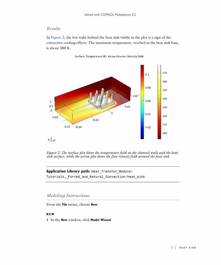
In Figure 2, the hot wake behind the heat sink visible in the plot is a sign of the convective cooling effects. The maximum temperature, reached at the heat sink base, is about 380 K.
Figure 2: The surface plot shows the temperature field on the channel walls and the heat sink surface, while the arrow plot shows the flow velocity field around the heat sink.
2 In the Select physics tree, select Heat Transfer>Conjugate Heat Transfer>Laminar Flow.
3 Click Add.
4 Click Study.
5 In the Select study tree, select Preset Studies for Selected Physics Interfaces>Stationary.
6 Click Done.
G E O M E T R Y 1
The model geometry is available as a parameterized geometry sequence in a separate MPH-file. If you want to build it from scratch, follow the instructions in the section Appendix: Geometry Modeling Instructions. Otherwise load it from file with the following steps.
1 On the Geometry toolbar, click Insert Sequence.
2 Browse to the application’s Application Library folder and double-click the file heat_sink_geom_sequence.mph.
The application’s Application Library folder is shown in the Application Library path section immediately before the current section. Note that the path given there is relative to the COMSOL Application Library root, which for a standard installation on Windows is C:\Program Files\COMSOL\COMSOL52\Multiphysics\applications.
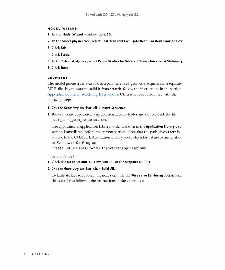
Import 1 (imp1)1 Click the Go to Default 3D View button on the Graphics toolbar.
2 On the Geometry toolbar, click Build All.
To facilitate face selection in the next steps, use the Wireframe Rendering option (skip this step if you followed the instructions in the appendix):
T S I N K
Solved with COMSOL Multiphysics 5.2
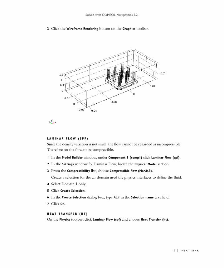
3 Click the Wireframe Rendering button on the Graphics toolbar.
L A M I N A R F L O W ( S P F )
Since the density variation is not small, the flow cannot be regarded as incompressible. Therefore set the flow to be compressible.
1 In the Model Builder window, under Component 1 (comp1) click Laminar Flow (spf).
2 In the Settings window for Laminar Flow, locate the Physical Model section.
3 From the Compressibility list, choose Compressible flow (Ma<0.3).
Create a selection for the air domain used the physics interfaces to define the fluid.
4 Select Domain 1 only.
5 Click Create Selection.
6 In the Create Selection dialog box, type Air in the Selection name text field.
7 Click OK.
H E A T TR A N S F E R ( H T )
On the Physics toolbar, click Laminar Flow (spf) and choose Heat Transfer (ht).
5 | H E A T S I N K
Solved with COMSOL Multiphysics 5.2
6 | H E A
Heat Transfer in Fluids 11 In the Model Builder window, under Component 1 (comp1)>Heat Transfer (ht) click
Heat Transfer in Fluids 1.
2 In the Settings window for Heat Transfer in Fluids, locate the Domain Selection section.
3 From the Selection list, choose Air.
M A T E R I A L S
Next, add materials.
A D D M A T E R I A L
1 On the Home toolbar, click Add Material to open the Add Material window.
2 Go to the Add Material window.
3 In the tree, select Built-In>Air.
4 Click Add to Component in the window toolbar.
M A T E R I A L S
Air (mat1)1 In the Model Builder window, under Component 1 (comp1)>Materials click Air (mat1).
2 In the Settings window for Material, locate the Geometric Entity Selection section.
3 From the Selection list, choose Air.
A D D M A T E R I A L
1 Go to the Add Material window.
2 In the tree, select Built-In>Aluminum 3003-H18.
3 Click Add to Component in the window toolbar.
M A T E R I A L S
Aluminum 3003-H18 (mat2)1 In the Model Builder window, under Component 1 (comp1)>Materials click Aluminum
3003-H18 (mat2).
2 Select Domain 2 only.
A D D M A T E R I A L
1 Go to the Add Material window.
T S I N K
Solved with COMSOL Multiphysics 5.2
2 In the tree, select Built-In>Silica glass.
3 Click Add to Component in the window toolbar.
M A T E R I A L S
Silica glass (mat3)1 In the Model Builder window, under Component 1 (comp1)>Materials click Silica glass
(mat3).
2 Select Domain 3 only.
3 On the Home toolbar, click Add Material to close the Add Material window.
Material 4 (mat4)1 In the Model Builder window, under Component 1 (comp1) right-click Materials and
choose Blank Material.
2 In the Settings window for Material, type Thermal Grease in the Label text field.
3 Locate the Geometric Entity Selection section. From the Geometric entity level list, choose Boundary.
4 Select Boundary 34 only.
5 Click to expand the Material properties section. Locate the Material Properties section. In the Material properties tree, select Basic Properties>Thermal Conductivity.
6 Click Add to Material.
7 Locate the Material Contents section. In the table, enter the following settings:
G L O B A L D E F I N I T I O N S
Parameters1 In the Model Builder window, expand the Global Definitions node, then click
Parameters.
2 In the Settings window for Parameters, locate the Parameters section.
3 In the table, enter the following settings:
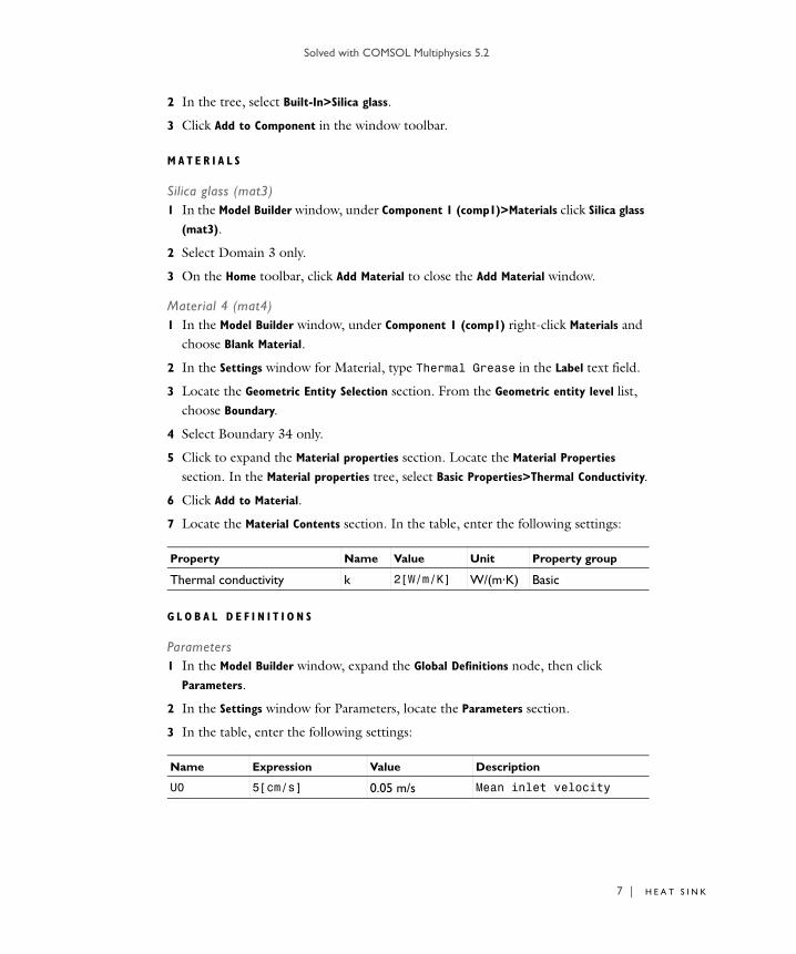
Property Name Value Unit Property group
Thermal conductivity k 2[W/m/K] W/(m·K) Basic
Name Expression Value Description
U0 5[cm/s] 0.05 m/s Mean inlet velocity
7 | H E A T S I N K
Solved with COMSOL Multiphysics 5.2
8 | H E A
Now define the physical properties of the model. Start with the fluid domain.
L A M I N A R F L O W ( S P F )
On the Physics toolbar, click Heat Transfer (ht) and choose Laminar Flow (spf).
The no-slip condition is the default boundary condition for the fluid. Define the inlet and outlet conditions as described below.
1 In the Model Builder window, under Component 1 (comp1) click Laminar Flow (spf).
Inlet 11 On the Physics toolbar, click Boundaries and choose Inlet.
2 Select Boundary 121 only.
3 In the Settings window for Inlet, locate the Boundary Condition section.
4 From the list, choose Laminar inflow.
5 Locate the Laminar Inflow section. In the Uav text field, type U0.
Outlet 11 On the Physics toolbar, click Boundaries and choose Outlet.
2 Click the Zoom Extents button on the Graphics toolbar.
3 Select Boundary 1 only.
H E A T TR A N S F E R ( H T )
Thermal insulation is the default boundary condition for the temperature. Define the inlet temperature and the outlet condition as described below.
1 In the Model Builder window, under Component 1 (comp1) click Heat Transfer (ht).
Temperature 11 On the Physics toolbar, click Boundaries and choose Temperature.
2 Select Boundary 121 only.
3 In the Settings window for Temperature, locate the Temperature section.
4 In the T0 text field, type T0.
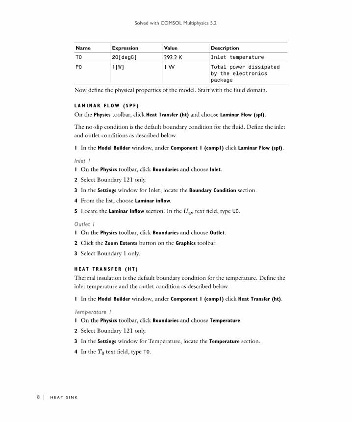
T0 20[degC] 293.2 K Inlet temperature
P0 1[W] 1 W Total power dissipated by the electronics package
Name Expression Value Description
T S I N K
Solved with COMSOL Multiphysics 5.2
Outflow 11 On the Physics toolbar, click Boundaries and choose Outflow.
2 Select Boundary 1 only.
Next, use the P0 parameter to define the total heat source in the electronics package.
Heat Source 11 On the Physics toolbar, click Domains and choose Heat Source.
2 Select Domain 3 only.
3 In the Settings window for Heat Source, locate the Heat Source section.
4 Click the Overall heat transfer rate button.
5 In the P0 text field, type P0.
Finally, add the thin thermal grease layer.
Thin Layer 11 On the Physics toolbar, click Boundaries and choose Thin Layer.
2 Select Boundary 34 only.
3 In the Settings window for Thin Layer, locate the Thin Layer section.
4 In the ds text field, type 50[um].
M E S H 1
1 In the Model Builder window, under Component 1 (comp1) click Mesh 1.
2 In the Settings window for Mesh, locate the Mesh Settings section.
3 From the Element size list, choose Extra coarse.
4 Click the Build All button.
To get a better view of the mesh, hide some of the boundaries.
5 Click the Click and Hide button on the Graphics toolbar.
6 Click the Select Boundaries button on the Graphics toolbar.
9 | H E A T S I N K
Solved with COMSOL Multiphysics 5.2
10 | H E
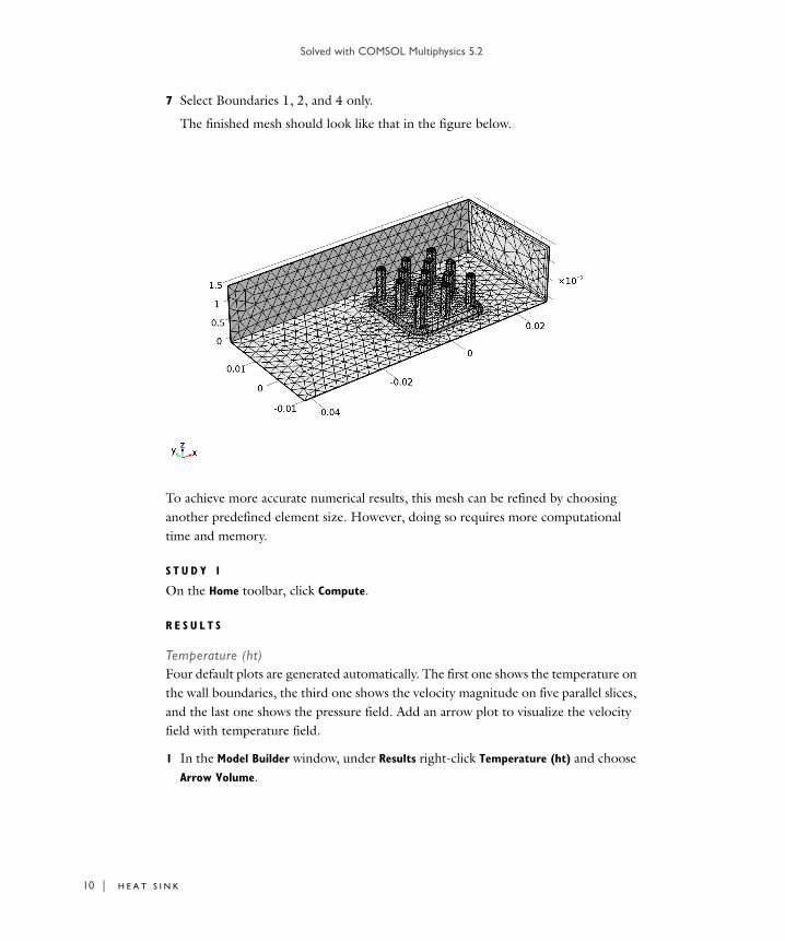
7 Select Boundaries 1, 2, and 4 only.
The finished mesh should look like that in the figure below.
To achieve more accurate numerical results, this mesh can be refined by choosing another predefined element size. However, doing so requires more computational time and memory.
S T U D Y 1
On the Home toolbar, click Compute.
R E S U L T S
Temperature (ht)Four default plots are generated automatically. The first one shows the temperature on the wall boundaries, the third one shows the velocity magnitude on five parallel slices, and the last one shows the pressure field. Add an arrow plot to visualize the velocity field with temperature field.
1 In the Model Builder window, under Results right-click Temperature (ht) and choose Arrow Volume.
A T S I N K
Solved with COMSOL Multiphysics 5.2
2 In the Settings window for Arrow Volume, click Replace Expression in the upper-right corner of the Expression section. From the menu, choose Component 1>Laminar
Flow>Velocity and pressure>u,v,w - Velocity field.
3 Locate the Arrow Positioning section. Find the x grid points subsection. In the Points text field, type 40.
4 Find the y grid points subsection. In the Points text field, type 20.
5 Find the z grid points subsection. From the Entry method list, choose Coordinates.
6 In the Coordinates text field, type 5[mm].
7 Right-click Results>Temperature (ht)>Arrow Volume 1 and choose Color Expression.
8 In the Settings window for Color Expression, click Replace Expression in the upper-right corner of the Expression section. From the menu, choose Component
1>Laminar Flow>Velocity and pressure>spf.U - Velocity magnitude.
9 On the Temperature (ht) toolbar, click Plot.
Global Evaluation 1On the Results toolbar, click Global Evaluation.
Derived Values1 In the Settings window for Global Evaluation, type Net Energy Rate in the Label
text field.
2 Click Replace Expression in the upper-right corner of the Expression section. From the menu, choose Component 1>Heat Transfer>Global>Net powers>ht.ntefluxInt -
Total net energy rate.
3 Click the Evaluate button.
TA B L E
Go to the Table window.
R E S U L T S
Global Evaluation 2On the Results toolbar, click Global Evaluation.
Derived Values1 In the Settings window for Global Evaluation, type Heat Source in the Label text
field.
11 | H E A T S I N K
Solved with COMSOL Multiphysics 5.2
12 | H E
2 Click Replace Expression in the upper-right corner of the Expression section. From the menu, choose Component 1>Heat Transfer>Global>Heat source powers>ht.QInt -
Total heat source.
3 Click the Evaluate button.
TA B L E
1 Go to the Table window.
The total rate of net energy and heat generation should be close to 1 W.
Appendix: Geometry Modeling Instructions
R O O T
On the Home toolbar, click Add Component and choose 3D.
G L O B A L D E F I N I T I O N S
First define the geometry parameters.
Parameters1 On the Home toolbar, click Parameters.
2 In the Settings window for Parameters, locate the Parameters section.
3 In the table, enter the following settings:
G E O M E T R Y 1
Build the geometry in three steps. First, import the heat sink geometry from a file.
Import 1 (imp1)1 On the Home toolbar, click Import.
2 In the Settings window for Import, locate the Import section.
3 Click Browse.
Name Expression Value Description
L_channel 7[cm] 0.07 m Channel length
W_channel 3[cm] 0.03 m Channel width
H_channel 1.5[cm] 0.015 m Channel height
L_chip 1.5[cm] 0.015 m Chip size
H_chip 2[mm] 0.002 m Chip height
A T S I N K
Solved with COMSOL Multiphysics 5.2
4 Browse to the application’s Application Library folder and double-click the file heat_sink.mphbin.
5 Click Import.
6 Click the Wireframe Rendering button on the Graphics toolbar.
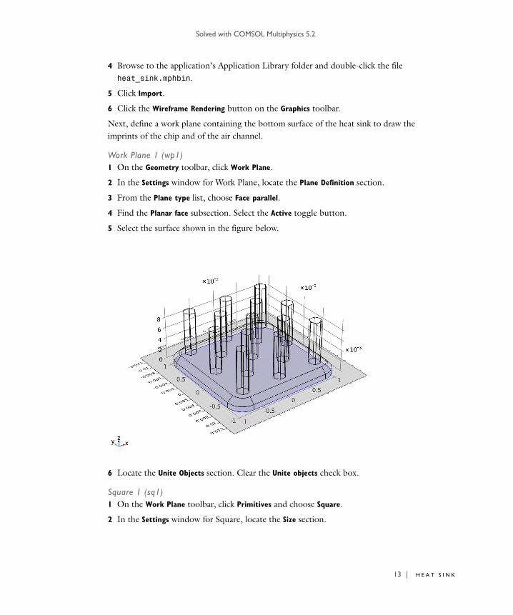
Next, define a work plane containing the bottom surface of the heat sink to draw the imprints of the chip and of the air channel.
Work Plane 1 (wp1)1 On the Geometry toolbar, click Work Plane.
2 In the Settings window for Work Plane, locate the Plane Definition section.
3 From the Plane type list, choose Face parallel.
4 Find the Planar face subsection. Select the Active toggle button.
5 Select the surface shown in the figure below.
6 Locate the Unite Objects section. Clear the Unite objects check box.
Square 1 (sq1)1 On the Work Plane toolbar, click Primitives and choose Square.
2 In the Settings window for Square, locate the Size section.
13 | H E A T S I N K
Solved with COMSOL Multiphysics 5.2
14 | H E
3 In the Side length text field, type L_chip.
4 Locate the Position section. From the Base list, choose Center.
5 Right-click Square 1 (sq1) and choose Build Selected.
6 Click the Zoom Extents button on the Graphics toolbar.
Rectangle 1 (r1)1 On the Work Plane toolbar, click Primitives and choose Rectangle.
2 In the Settings window for Rectangle, locate the Size and Shape section.
3 In the Width text field, type L_channel.
4 In the Height text field, type W_channel.
5 Locate the Position section. In the xw text field, type -45[mm].
6 In the yw text field, type -W_channel/2.
7 Right-click Rectangle 1 (r1) and choose Build Selected.
Now extrude the chip imprint to define the chip volume.
Extrude 1 (ext1)1 On the Geometry toolbar, click Extrude.
2 Select the object wp1.sq1 only.
3 In the Settings window for Extrude, locate the Distances from Plane section.
4 In the table, enter the following settings:
5 Right-click Extrude 1 (ext1) and choose Build Selected.
6 Click the Zoom Extents button on the Graphics toolbar.
To finish the geometry, extrude the channel imprint in the opposite direction to define the air volume.
Extrude 2 (ext2)1 On the Geometry toolbar, click Extrude.
2 Select the object wp1.r1 only.
3 In the Settings window for Extrude, locate the Distances from Plane section.
Distances (m)
H_chip
A T S I N K
Solved with COMSOL Multiphysics 5.2
4 In the table, enter the following settings:
5 Select the Reverse direction check box.
6 Click the Build All Objects button.
7 Click the Zoom Extents button on the Graphics toolbar.