ORIGINAL RESEARCH PAPER Solvency II solvency capital requirement for life insurance companies based on expected shortfall Tim J. Boonen 1 Received: 16 March 2015 / Revised: 22 May 2017 / Accepted: 10 July 2017 / Published online: 14 October 2017 Ó The Author(s) 2017. This article is an open access publication Abstract This paper examines the consequences for a life annuity insurance company if the solvency II solvency capital requirements (SCR) are calibrated based on expected shortfall (ES) instead of value-at-risk (VaR). We focus on the risk modules of the SCRs for the three risk classes equity risk, interest rate risk and longevity risk. The stress scenarios are determined using the calibration method proposed by EIOPA in 2014. We apply the stress-scenarios for these three risk classes to a fictitious life annuity insurance company. We find that for EIOPA’s current quantile 99.5% of the VaR, the stress scenarios of the various risk classes based on ES are close to the stress scenarios based on VaR. Might EIOPA choose to calibrate the stress scenarios on a smaller quantile, the longevity SCR is relatively larger and the equity SCR is relatively smaller if ES is used instead of VaR. We derive the same conclusion if stress scenarios are determined with empirical stress scenarios. Keywords Solvency II Solvency capital requirement Expected shortfall Value-at-risk 1 Introduction Solvency II is the new supervisory framework that is in force from 2016 for insurers and reinsurers in Europe. It puts demands on the required economic capital, risk management, and reporting standards of insurance companies. Solvency II focuses on an enterprize risk management approach towards required capital standards. Its & Tim J. Boonen [email protected]1 Amsterdam School of Economics, University of Amsterdam, Roetersstraat 11, 1018 WB Amsterdam, The Netherlands 123 Eur. Actuar. J. (2017) 7:405–434 https://doi.org/10.1007/s13385-017-0160-4
Transcript
ORIGINAL RESEARCH PAPER
Solvency II solvency capital requirement for lifeinsurance companies based on expected shortfall
Tim J. Boonen1
Received: 16 March 2015 / Revised: 22 May 2017 / Accepted: 10 July 2017 /
Published online: 14 October 2017
� The Author(s) 2017. This article is an open access publication
Abstract This paper examines the consequences for a life annuity insurance
company if the solvency II solvency capital requirements (SCR) are calibrated
based on expected shortfall (ES) instead of value-at-risk (VaR). We focus on the
risk modules of the SCRs for the three risk classes equity risk, interest rate risk and
longevity risk. The stress scenarios are determined using the calibration method
proposed by EIOPA in 2014. We apply the stress-scenarios for these three risk
classes to a fictitious life annuity insurance company. We find that for EIOPA’s
current quantile 99.5% of the VaR, the stress scenarios of the various risk classes
based on ES are close to the stress scenarios based on VaR. Might EIOPA choose to
calibrate the stress scenarios on a smaller quantile, the longevity SCR is relatively
larger and the equity SCR is relatively smaller if ES is used instead of VaR. We
derive the same conclusion if stress scenarios are determined with empirical stress
scenarios.
Keywords Solvency II � Solvency capital requirement � Expectedshortfall � Value-at-risk
1 Introduction
Solvency II is the new supervisory framework that is in force from 2016 for insurers
and reinsurers in Europe. It puts demands on the required economic capital, risk
management, and reporting standards of insurance companies. Solvency II focuses
on an enterprize risk management approach towards required capital standards. Its
main objective is to ensure that insurance companies hold sufficient economic
capital to protect the policyholders as it aims to reduce the risk that an insurer is
unable to meet its financial claims (see, e.g., [17]). The required capital is based on
the risks that the insurer faces. This capital requirement is called the solvency
capital requirement (SCR) and covers all the risks that an insurer faces. EIOPA [25]
defines the SCR of an insurance or reinsurance company as the value-at-risk (VaR)
of the basic own funds subject to a confidence level of 99.5% on a 1-year period. In
this paper, we base our model on the solvency II calibrations of EIOPA [25, 26].
The value-at-risk is a widely used risk measure and can be described as the
maximum loss within a certain confidence level. In the case of the SCR, the
confidence level of 99.5% tells us that the company can expect to lose no more than
VaR in the next year with 99.5% confidence, so, on average, only once every
200 years the VaR loss level will be exceeded. The value-at-risk is however
criticized for not being sub-additive [4]. Sub-additivity of a risk measure ensures
that diversification is rewarded. Besides not being sub-additive, the VaR does also
not consider the shape of the tail beyond the confidence level. This means that the
VaR does not take into account what happens beyond the confidence level, so it
does not consider the worst case scenarios. This is discussed by Acerbi and Tasche
[3] and Yamai and Yoshiba [46]. The fact that VaR is not sub-additive and that it
does not consider the tail beyond the confidence level might make it less suitable to
calculate capital requirements.
Coherent risk measures are sub-additive, and consider the shape of the tail
beyond the confidence level. A risk measure is called coherent if it satisfies the
axioms translation invariance, sub-additivity, positive homogeneity, and mono-
tonicity [4]. The most popular coherent risk measure is the expected shortfall (ES).
This risk measure is equal to the expected value of the loss, given that the loss is
larger than the value-at-risk, therefore the expected shortfall also depends on the
quantile used. Two other regulatory frameworks for financial institutions, the Swiss
Solvency Test and the Basel III framework, use the expected shortfall as risk
measure.
The contribution of this paper is not to claim that the expected shortfall is a better
risk measure than the value-at-risk. Instead, we exemplary analyze the effects on
three main risk factors of the total SCR for a fictitious life annuity insurer if the
solvency II SCR calibration is based on expected shortfall instead of value-at-risk.
The use of expected shortfall for insurance stress testing is also suggested by
CEIOPS [12], Sandstrom [40], and Wagner [45]. We hereby consider this
hypothetical change in regulation for three major risk classes: equity risk, interest
rate risk, and longevity risk. Moreover, we analyze what happens if all SCRs are
determined via empirical stress scenarios.
The standard model of solvency II explicitly assumes a Gaussian distribution for
returns in some risk classes. If a return is Gaussian, the value-at-risk, as prescribed
by solvency II, and expected shortfall provide similar information (e.g., [46]). If
returns are non-Gaussian, which is observed for the most important classes of risk,
the use of value-at-risk might lead to a mismatch of the SCR and the underlying
riskiness. In this paper, we examine what the effects are of using such a standard
model when risks are calibrated using the expected shortfall instead. We find that
406 T. J. Boonen
123
for EIOPA’s current quantile 99.5% of the value-at-risk, the stress scenarios of the
various risk classes based on expected shortfall are close to the stress scenarios
based on value-at-risk. We show that if EIOPA aims to keep the solvency capital
requirement the same if it would switch to v, it should set the confidence level at
approximately 98.8%. So, applying a 99% confidence level for the expected
shortfall leads to an increase in the solvency capital requirement. Moreover, might
EIOPA choose to calibrate the stress scenarios on a smaller quantile, the longevity
SCR is relatively large and the equity SCR is relatively small if expected shortfall is
used instead of value-at-risk.
This paper is set out as follows. Section 2 defines the risk measures value-at-risk
and expected shortfall. Section 3 introduces the part of the solvency II regulations
that we use in this paper. Section 4 states our methodology, and shows the stress
scenarios for the solvency capital requirements under the two risk measures.
Section 5 shows the main results, and a sensitivity analysis. Section 6 illustrates our
results in relations to other regulatory frameworks, and Sect. 7 concludes.
2 Risk measures to calibrate solvency capital
Risk measures are used to determine the amount of economic capital to be kept in
reserve in order to protect a company for any negative risky impacts that may arise
in the future. A risk measure maps random variables into real numbers. In this paper
we discuss two well known risk measures: the value-at-risk (VaR) and the expected
shortfall (ES), where we refer to McNeilet al. [36] for more details about these two
risk measures.
The value-at-risk with confidence level a 2 ð0; 1Þ is the a-quantile, i.e.,
VaRaðXÞ ¼ inffx 2 IR : PðX[ xÞ� 1� ag; ð1Þ
for all random variables X (a loss).
Coherence of risk measures is introduced by Artzner et al. [4]. A risk measures qis coherent if it satisfies the four axioms translation invariance, sub-additivity,
positive homogeneity, and monotonicity. The relevance of these properties is widely
discussed by Artzner et al. [4]. Particularly, sub-additivity of a risk measure implies
that the risk measure weakly decreases if risks are pooled. It also implies that there
is no incentive for a company to split its risk into pieces and evaluate them
separately.
The expected shortfall (ES) is given by
ESaðXÞ ¼1
1� a
Z 1
aVaRsðXÞds; ð2Þ
for all a 2 ½0; 1Þ, and all random variables X (a loss), whenever the integral con-
verges. If the integral does not converge, ES equals infinity. An infinite value of a
risk measure is useless for practical purposes. If the random variable X is contin-
uously distributed, the ES may be even more intuitively expressed as conditional
VaR or the tail conditional expectation:
Solvency II solvency capital requirement for life insurance companies... 407
123
ESaðXÞ ¼ EðX j X�VaRaðXÞÞ: ð3Þ
For numerical convenience, the expression in (3) is often used in historical simu-
lations. For the same reason, we use (3) as definition of expected shortfall in this
paper.
The use of expected shortfall gained popularity (see, e.g., [1, 20]). The main
argument is based on the fact that ES considers the size of worst case events,
whereas the VaR uses only a quantile. A quantile provides insight in the frequency
of worst case events, where the ES considers both the frequency and size. For this
reason, the interpretation of the ES is not straightforward. Other arguments in favor
of the ES are based on stability and robustness (see, e.g., [33]). Danielsson et al. [16]
show that the sub-additivity may be violated if historical simulations are used.
Historical simulations are used in the calibration of solvency II. Other authors that
claim that the ES is more appropriate to determine capital buffers are Beder [10],
Acerbi and Tasche 3, [44], Frey and McNeil [28], Yamai and Yoshiba [46], and
Wagner [45]. CEIOPS [12] acknowledges the theoretical advantages of using the
expected shortfall to calculate the SCR.
On the other hand, backtesting of the VaR is relatively straightforward compared
to the ES (see, e.g., [2]). Kellner and Rosch [32] show that the ES is more sensitive
to model risk than the VaR. Koch-Medina and Munari [34] show that the ES does
not protect the policyholders sufficiently. Moreover, in the literature, the relevance
of coherence (and sub-additivity) is criticized as well (see, e.g., [9, 35]). To
summarize, there is no clear argument whether the ES is better than the VaR. This
paper does not aim to provide a justification for either of the two risk measures, but
seeks to compare them quantitatively in the solvency II context.
When returns are Gaussian, the same information is given by the value-at-risk
and expected shortfall. In particular, the value-at-risk and expected shortfall are
multiples of the standard deviation for zero-mean Gaussian random variables. For
example, VaR at 99.5% confidence level is approximately 2.58 times the standard
deviation, while expected shortfall at the same confidence level is approximately
2.89 times the standard deviation.1 The assumption that financial returns are
Gaussian is often criticized and it may lead to an underestimation of the risk being
faced (see, e.g., [40]). It is a well-known (e.g., [14]) that asset returns are fat-tailed,
asymmetric and, therefore, not Gaussian.
3 Solvency II
We describe the solvency II regulations in Sect. 3.1. In Sect. 3.2, we specify all
formulas of the solvency capital requirements (SCR) according to EIOPA [25] for
three relevant risk classes.
1 As shown by Yamai and Yoshiba [46], it holds that if the random variable X is Gaussian with mean land standard deviation r, then VaRaðXÞ ¼ lþ qar and EShðXÞ ¼ lþ ½/ðqhÞ=ð1� hÞ�r, where qa is thequantile-function of a standard Gaussian distribution, and / is the density function of a standard Gaussian
distribution.
408 T. J. Boonen
123
3.1 Introduction
Solvency II is a regulatory framework that is in force since 2016 for the European
insurance industry and puts demands on the required economic capital, risk
management and reporting standards of insurance companies. The underlying
quantitative regulation mechanism is that insurers should hold an amount of capital
that enables them to absorb unexpected losses and meet the obligations towards
policyholders at a high level of equitableness. In the European Union, there are on-
going discussions about applying such a framework to all European pension funds
as well [23]. For instance, see Doff [17], Eling et al. [19], Sandstrom [40], Steffen
[43], and Wagner [45] for an overview and critical discussion of the solvency II
framework.
This paper focusses on the first pillar of the solvency II framework. This pillar
prescribes the quantitative requirements which an insurer must meet. It contains the
SCR, which is to be calculated by using the standard formula or an internal model or
a combination of the two. These quantitative requirements are supported by the so-
called quantitative impact studies (QIS). For internal models, it is also not clear how
the SCR is precisely defined [11] and therefore we focus on the standard formula in
this paper.
EIOPA [25] describes how the assets and liabilities of an insurer should be
valued. Assets should be valued at the amount for which they could be exchanged
between knowledgeable willing parties in an arm’s length transaction. Liabilities
should be valued at the amount for which they could be transferred, or settled,
between parties in an arm’s length transaction. Valuing assets on a market-
consistent basis is generally straightforward. Generally, perfect replication of
expected cash flows is not possible for the liabilities of an insurer. The quantitative
impact study 5 (QIS 5) prescribes to use the best estimate and the risk margin to
value the liabilities. The best estimate of the liabilities (BEL) is the present value of
the expected future liability payments. The risk margin is the cost of holding an
amount of basic own funds equal to the SCR over the lifetime of the insurance
liabilities.
EIOPA [25] prescribes that the SCR should correspond to the value-at-risk of the
basic own funds of an insurer subject to a confidence level of 99.5% on a 1-year
period. The principle of the standard formula is to apply a set of shocks to certain
risk drivers, and to calculate the impact on the basic own funds for various risks.
These shocks are calibrated using the VaR with a confidence level of 99.5%. The
standard formula of the SCR is divided into risk modules. Predefined correlation
matrices are used to aggregate the SCRs for all risks to the total SCR.
We do not consider operational risk, and the adjustment for the risk absorbing
effects of technical provisions and deferred taxes. Moreover, we only consider
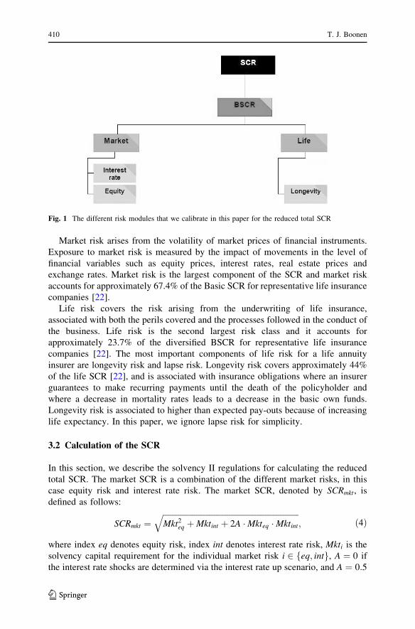
equity risk, interest rate risk and longevity risk. In Fig. 1, we provide an overview of
our reduced total SCR calculation and its different risk modules. Market risk and
life risk account together for approximately 91.1% of the basic SCR for life
insurance companies [22]. Moreover, EIOPA [24] shows that the market risk
predominantly consists of equity and interest rate risk.
Solvency II solvency capital requirement for life insurance companies... 409
123
Market risk arises from the volatility of market prices of financial instruments.
Exposure to market risk is measured by the impact of movements in the level of
financial variables such as equity prices, interest rates, real estate prices and
exchange rates. Market risk is the largest component of the SCR and market risk
accounts for approximately 67.4% of the Basic SCR for representative life insurance
companies [22].
Life risk covers the risk arising from the underwriting of life insurance,
associated with both the perils covered and the processes followed in the conduct of
the business. Life risk is the second largest risk class and it accounts for
approximately 23.7% of the diversified BSCR for representative life insurance
companies [22]. The most important components of life risk for a life annuity
insurer are longevity risk and lapse risk. Longevity risk covers approximately 44%
of the life SCR [22], and is associated with insurance obligations where an insurer
guarantees to make recurring payments until the death of the policyholder and
where a decrease in mortality rates leads to a decrease in the basic own funds.
Longevity risk is associated to higher than expected pay-outs because of increasing
life expectancy. In this paper, we ignore lapse risk for simplicity.
3.2 Calculation of the SCR
In this section, we describe the solvency II regulations for calculating the reduced
total SCR. The market SCR is a combination of the different market risks, in this
case equity risk and interest rate risk. The market SCR, denoted by SCRmkt, is
where an implicit assumption is that the correlation between ‘‘global’’ and ‘‘other’’
equity is 0.75.
To determine the solvency capital requirement for interest rate risk, an upward
and a downward shock are given to the interest term structure. The altered term
structures are given by maxfð1þ supm Þ � rm; rm þ 1%g and ð1þ sdownm Þ � rm, where rmis the current interest rate with maturity m, and supm and sdownm are the up- and down-
shocks to the interest rates with maturity m. These shocks to the interest rates are
expressed as the relative amounts compared to the current interest rates. So, in
addition to the calibration of the relative stress factor, a minimum shock of 1% is
applied for the interest rate in the upward scenario [26]. Using an alternative term
structure results in a change of the value of the assets and liabilities. The solvency
capital requirements for the downward and upward shock are determined by the
changes in the BOF if the shocked interest rate curve is used instead of the nominal
term structure. The interest rate shock is the worst of the up and down shock. This
leads to the following definitions:
Mktup;int ¼ MBOFjupshock; ð7Þ
Mktdown;int ¼ MBOFjdownshock; ð8Þ
Mktint ¼ maxfMktup;int;Mktdown;int; 0g: ð9Þ
In this paper, we only consider longevity risk in the class of life risk, i.e., the life
SCR equals longevity SCR. The longevity SCR is determined by the change in net
2 Adding a risk margin (based on the total SCR) would lead to a circular argument. This is noted by
Coppola and D’Amato [15].
Solvency II solvency capital requirement for life insurance companies... 411
123
value of assets minus liabilities after a permanent percentage decrease in mortality
rates for all ages. This decrease resembles the risk that people live longer than
expected and this leads to an increase in the present value of the liabilities from
annuity products. This shock therefore leads to a decrease in the value of BOF. The
where SCRi is the solvency capital requirement for the individual risk class
i 2 fmkt; lifeg, and where an implicit assumption is that the correlation between
market risk and life risk is 0.25.
The structure of the solvency capital requirements in solvency II is partially
derived from a formula developed by the German Insurance Association (see, e.g.,
[19, 41]). The structure of a square-root formula as in (4), (6) and (11) is derived
from the assumption that the individual returns are Gaussian and the dependence is
linear. In general, linear dependence is sufficient to describe dependencies between
elliptical distributions. However, there arise problems with this formula if the
individual returns are not Gaussian, or dependencies are non-linear. For instance,
skewness or excess kurtosis of the marginal distributions may lead to very irregular
outcomes (see [40]). Moreover, even if the different returns have Gaussian marginal
distributions, their influence on the aggregate loss may not be closely related to a
square-root formula (see [7]). Non-linear dependence structures may yield situations
where the square-root formula severely underestimates the total risk (see [38]). A
more accurate approach instead of the square-root formula may require nested
simulations, and is therefore substantially more complex (see [8]). In this paper, we
do not analyze alternative risk aggregation methods.
4 Methodology
In this section, we calibrate the SCR stress scenarios for the three risk classes based
on the VaR and the ES following the calibration methods used in solvency II. We
calculate the SCR with stress scenarios calibrated with VaR or ES for a fictitious life
annuity insurer. To show the impact of the stress scenarios on this life annuity
insurer, we first specify the insurer in Sect. 4.1. In Sect. 4.2, we introduce the
method we use to compare the stress scenarios based on VaR with the stress
scenarios based on ES. In Sect. 4.3, we show the stress scenarios for all three risk
classes.
412 T. J. Boonen
123
4.1 Calibrating the fictitious life annuity insurer
The liability portfolio of the fictitious insurer consists of (deferred) life annuity
products only. The portfolio is normalized such that it consists of 100,000 male
policyholders. The policyholders in this portfolio have an average age of 50 years.
In Table 7 in Appendix 1, we provide details of the liability portfolio.
The single-life annuity will be paid at the end of every year starting from age 65
if alive. So, for policyholders younger than age 65, it is a deferred annuity. For the
youngest age cohort 21, the yearly amount paid out after age 65 is equal to 0.067.
This amount increases linearly over the age cohorts up to 1 for age cohorts of 65
years old and older. The increasing trend accounts for the fact that younger cohorts
have paid less premiums in the past. Here, we use age 65 as a retirement age, where
the retirement benefits are normalized to 1 for every retired individual. We refer to
Hari et al. [29] for an overview of the actuarial valuation of the annuity liabilities.
To discount cash flows and determine the bond prices, we use the nominal
interest rate term structure of the European central bank and a Smith–Wilson
extrapolation [42] towards an ultimate forward rate (UFR) for interest rates after 20
years (see Fig. 7 in Appendix 1).3 We set the present at December 31st, 2014.
We assume that the fictitious insurer has no BOF, so the asset value is equal to
the value of the liabilities. The asset portfolio consists of 25% in ‘‘global’’ equity
and 75% in bonds. To construct the bond portfolio, we pick 5- and 30-year bonds.4
The 5-year bond has 2.13% coupons, and the 30-year bond has 3.45% coupons.5 We
determine the bond portfolio as follows. The duration of the bonds equals 50% of
the duration of the liabilities. Since 75% of the assets is invested in bonds, this
coincides with a duration of the assets of 75%� 50% ¼ 37:5% of the duration of
the liabilities. Via this duration, we determine the amount invested in the 5- and
30-year bonds. For both the characteristics of the portfolio and the composition of
the asset portfolio, we will later perform a sensitivity analysis. We use the mortality
table of the Dutch Actuarial Society: AG 2012-2062,6 developed in 2012, which
contains a longevity trend. Note that there is no risk involved in equity, interest rates
and longevity other then the stress scenarios.
4.2 Matching the total SCR value
For the fictitious life annuity insurer, we denote the SCR based on stress scenarios
calibrated on VaR and ES by SCR(VaRa) and SCR(ESh), for different parameters aand h. We focus on the relative impact on the SCR for the three risk classes.
3 See http://www.toezicht.dnb.nl/en/binaries/51-226788.pdf (last accessed: November 9th, 2016) or [13]
for more information on the procedure to calibrate the interest rate term structure.4 For EEA government bonds that have a AAA credit rating, an insurer is not required to hold an SCR for
spread risk by EIOPA [21].5 The coupon rates are based on the 5- and 30-year UK Gilt bonds on December 31st, 2014.6 For the detailed mortality table that we use, see http://www.ag-ai.nl/download/14127-
Prognosetafel?AG2012-2062.xls (last accessed: May 4th, 2017).
Solvency II solvency capital requirement for life insurance companies... 413
Therefore, to compare the SCR(VaRa) properly with the SCR(ESh), the confidence
level for the ES, h, is chosen based on matching the reduced total SCR value, i.e.,
SCRðVaRaÞ ¼ SCRðEShÞ: ð12Þ
In this way, we define the function h : ½95%; 100%� ! ½0; 1� as a strictly increasing
function such that (12) is satisfied for all a 2 ½95%; 100%�. For instance, we find thathð99:5%Þ � 98:78% and hð98:5%Þ � 97:00% if we calibrate the SCR risk scenarios
as we will specify in Sect. 4.3. We display the function h in Fig. 2. We get that the
function h is not affine, which is due to non-Gaussianity of the returns.7
Using the function h in (12), we compare the stress scenarios for equity risk,
interest rate risk and longevity risk. Those stress scenarios lead to three SCRs,
which are then used to determine the reduced total SCR as described in Sect. 3.2.
We denote the vector of the SCRs for all three risk classes as an allocation.
4.3 Calibrating the SCR stress scenarios
In this section, we calibrate stress scenarios for equity risk, interest rate risk, and
longevity risk based on the value-at-risk and the expected shortfall. After we
calibrate the distribution of the risks, we derive stress scenarios based on the VaR
and ES. These stress scenarios will be applied to the representative life annuity
insurer in Sect. 5. EIOPA [26] proposes stress scenarios given by a shock of the
Fig. 2 The function h as defined in Sect. 4.2
7 If all returns were Gaussian, we would have hð99:5%Þ � 98:71%. A commonly used rule of thumb is
that VaRa ¼ ESh, where h � 1� 2:5ð1� aÞ for large values of a. The Basel III regulation moves for
instance from a VaR with a ¼ 99% to an ES with h ¼ 97:5%. In Fig. 2, we see that this relation holds for
smaller quantiles a, but the factor 2 (instead of 2.5) provides a better representation for large quantiles.
So, if an ES with h ¼ 99% is used instead of a VaR with a ¼ 99:5%, the reduced total SCR increases.
414 T. J. Boonen
123
underlying risk. This risk may be multi-dimensional, which is the case for interest
rate risk. Interest rate SCR is calculated via shocks for every duration (see (7)–(9)).
In line with this approach of EIOPA, we assume that the SCR for a risk is given by
shocki ¼ qðriskiÞ; i ¼ 1; . . .; I;
SCR ¼ DBOFjshock;
where q is the risk measure VaR or ES, and the dimension of the risk is I. The data
we use in this paper to calibrate the distribution of the risks is similar to the data
used of CEIOPS [13] and EIOPA [26], except that we modify the horizons.
The calibration method for equity risk is discussed by CEIOPS [13]. The
empirical distribution of annual holding period returns is derived from the Morgan
Stanley Capital International (MSCI) World Developed (Market) Price Equity
Index. The data from Bloomberg consists of daily returns for a period of 41 years,
starting in June 1973 until June 2014. We convert this into annual holding period
returns for every working day, with an overlapping horizon. The empirical VaR and
the empirical ES serve as the stress shock for ‘‘global’’ equity. We follow the
technical specifications of EIOPA [25] with an adjustment of 7.5% to increase the
equity risk shock. With this symmetric adjustment included, the stress rates for
equity risk are provided in Table 1. Recall that the function hðaÞ is fixed such that
the reduced total SCR remains the same. If a ¼ 99:5%, the differences between
using VaR and ES are small. When the quantile a ¼ 98:5% is chosen, the use of
VaR leads to a larger equity risk shock.
For the calibration method for interest rate risk, we use the following four
datasets as also used by CEIOPS [13] and EIOPA [26], but with shifted horizons in
order to include more recent data:
• Euro area government bond yield curve, with maturities from 1 to 15 years,
spaced out in annual intervals. The daily data spans a period of approximately
10 years and runs from September 2004 to July 2014. The data is from the
European Central Bank;8
• the UK government liability curve. The data is daily and is from the Bank of
England.9 The data covers a period from January 1998 to June 2014, so that the
longer maturities (i.e., beyond 15 years) are all available. It contains rates of
maturities starting from 1 year up until 20 year whilst the in between data points
are spaced on annual intervals;
• Euro vs Euribor IR swap rates. The daily data is downloaded from Datastream
and covers a period from 1999 to 2014. The data contains the 1–10 year rates
spaced out in 1-year intervals, as well as the 12, 15 and 20 year rates;
• UK (GBP) 6m IRS swap rates. The daily data is downloaded from Datastream
and covers a period from 1999 to 2014. The data contains the 1–10 year rates
spaced out in 1-year intervals, as well as the 12, 15 and 20 year rates.
8 See https://www.ecb.europa.eu/stats/services/sdmx/html/index.en.html (last accessed: May 4th, 2017).9 See http://www.bankofengland.co.uk/statistics/yieldcurve/archive.htm (last accessed: May 4th, 2017).
Solvency II solvency capital requirement for life insurance companies... 415
The data sets represent the most liquid markets for interest rate-sensitive
instruments in the European area. These four datasets are used to determine the
risk in interest rates, that we will use to determine the stress scenarios.
We calibrate the stress interest rate scenarios using principal component analysis
(PCA) as prescribed by EIOPA [26]. To transform the principal components and
eigenvectors into a VaR and an ES, we use the method described by Fiori and
Iannotti [27]. We describe and discuss the method we use in Appendix 2. For every
dataset, we derive a shock scenario for the annualized interest rate returns. So, we
have four stress shocks for every maturity from 1 to 20 years. For each maturity, the
overall interest rate shock is the average of the four stress shocks.
In Table 2, we provide the resulting stress scenarios of interest rates with
quantiles a ¼ 98:5; 99:5% for various maturities. Similar as for equity risk, the
differences between using VaR and ES are small when a ¼ 99:5%. Even though the
differences are small, calibrating with VaR leads to larger stress rates. When the
quantile a ¼ 98:5% is chosen, the differences are larger. We get for the fictitious
insurer that the down-shock is more harmful than the up-shock. This is partially due
to the fact that duration is not fully hedged.10 Hence, the down-shock is generally
used for the interest rate SCR.
We follow the calibration method for longevity shocks as introduced by CEIOPS
[13]. From the Human Mortality Database, we use unisex mortality tables from
1992 until 2009 with age bands of 5 years from nine countries. These nine countries
are Denmark, France, England and Wales, Estonia, Italy, Sweden, Poland, Hungary,
and Czech Republic. We calibrate the longevity stress scenarios by assuming that
annual mortality rate improvements follow a Gaussian distribution as prescribed by
CEIOPS [13]. The same shock in mortality rates is used for all different ages.
Annual mortality rate changes are calculated per country, per age band and per
year based on the data from the Human Mortality Database. We compute the means
and standard deviations of the annual mortality rate improvements, and we assume
that all annual mortality rate improvements have a Gaussian distribution. In this
case we have 198 Gaussian distributions, since we have nine countries and 22
different age bands. CEIOPS [13] determines per age cohort an average longevity
shock over all nine countries. This is than summarized into a longevity shock for all
age cohorts. We propose to determine the average of all age cohorts to determine the
age-independent longevity shock. So, we take the average of all VaRs or ESs. Due
to the Gaussian distribution of mortality improvements, we could define hanalytically for every a such that SCRlifeðVaRaÞ ¼ SCRlifeðEShÞ for any insurance
Table 1 Stress scenarios for ‘‘global’’ equity risk derived from the VaR and ES, where a fixed symmetric
adjustment of 7.5% is included
a (%) VaRa (%) EShðaÞ (%)
99.5 - 51.66 - 51.69
98.5 - 46.75 - 45.22
10 If the fictitious life annuity insurer applies duration matching, we still find that the down-shock is more
harmful than the up-shock.
416 T. J. Boonen
123
portfolio. Differences in the longevity SCR are due to the function h which may
differ from h.We display the stress scenarios for longevity risk in Table 3. For both quantiles
a ¼ 98:5; 99:5%, calibrating with ES leads to fiercer shock rates. The effect is larger
when the quantile a ¼ 98:5% is used.
When we apply the stress scenarios, we obtain that the reduced total SCR of the
fictitious life annuity insurer is approximately 23:24% of the BEL. The allocation of
this SCR(VaR99:5%) to the three different risk classes in shown in Table 4. In Fig. 3
we display SCR(VaRa) and SCR(ESa). By construction, it holds that
SCRðVaRaÞ� SCRðESaÞ.
Table 2 Interest rate stress scenarios supm and sdownm for maturities m ¼ 1; . . .; 20, calibrated with VaR99:5%,
The stress scenarios are then applied to the assets and liabilities of the fictitious life annuity insurer as
described in Sect. 3.2
Table 3 Stress rates for longevity risk derived from the VaR and ES
a (%) VaRa (%) EShðaÞ (%)
99.5 - 18.78 - 18.90
98.5 - 16.19 - 16.90
Solvency II solvency capital requirement for life insurance companies... 417
123
5 Results
In Sect. 5.1, we compare the allocation of SCR(VaRa) with the allocation of
SCR(EShðaÞ for a fictitious life annuity insurer. In Sect. 5.2, we provide some
sensitivity analysis and show that the results of Sect. 5.1 are robust to changes to the
asset and liability portfolio of the fictitious life annuity insurer.
5.1 Comparing the SCR(VaRa) with the SCR(EShðaÞ) for the fictitious life
annuity insurer
In this section, we compare the SCR(VaRa) with the SCR(EShðaÞ) for the fictitious
life annuity insurer. Recall that h is chosen such that SCR(VaRa) equals SCR(ESh).
Therefore, we focus on the allocation of the reduced total SCR for the three risk
classes: equity SCR, interest rate SCR and longevity SCR. By comparing these
allocations for VaR and ES, we can see whether the current method, which uses
VaR, underestimates or overestimates certain risks. This is done for different
quantiles a used for the VaR.
Table 4 The allocation of this SCR(VaR99:5%) for the fictitious life annuity insurer
Reduced total SCR 23.24%
Interest rate SCR 10.05%
Equity SCR 14.85%
Market SCR 21.70%
Longevity SCR 4.49%
All SCRs are expressed in percentage of the BEL
Fig. 3 Comparing SCR(VaRa) with SCR(ESa) of the fictitious life annuity insurer for various a
418 T. J. Boonen
123
5.1.1 The changes in allocation of the reduced total SCR
Figure 4 shows the change in allocation of the reduced total SCR for the three
different risk classes when ES is used to calibrate the shock scenarios instead of
VaR. The stress scenarios used to determine the SCR are derived as prescribed by
EIOPA, that means that the interest rate stress scenarios are calibrated using PCA
and the longevity stress scenarios are calibrated assuming Gaussian distributions.
We call this the base case.
Figure 4 shows for the quantile a ¼ 99:5% that the differences in allocation are
small. When the quantile a decreases to 98.5%, the differences become more
significant. By using ES to determine the shocks, the longevity risk and the interest
rate shocks are more harmful and the equity risk shock is milder. When we use ES
instead of VaR to determine the stress shocks for a ¼ 98:5%, the longevity SCR
grows with 4.22%, the interest rate SCR increases with 2.27%, and the equity SCR
decreases with 1.77%.
These changes do not add up to zero since the amounts of SCR for the different
risk measures differ. Therefore, a decrease of 2% for the equity SCR leads to a
larger change in the actual amount of SCR than an increase of 2% for the interest
rate SCR, because the equity SCR is larger than the interest rate SCR. When the
quantile a is smaller than 98.5%, the differences are smaller. For values of a smaller
than 97.5%, we get that the equity SCR is relatively large. This follows from the
observation that the tails for equity returns are fat (see, e.g., [14]), but the extreme
events are worse for the interest rate shocks. We get that relative effects are fairly
constant when a gets smaller, as tail risk events will have a smaller impact on both
the ES as the VaR.
Fig. 4 Comparing the allocation of SCR(VaRa) with the allocation of SCR(EShðaÞ) for the fictitious life
annuity insurer, when the stress scenarios are determined in a similar way as EIOPA prescribes (basecase). The horizontal axis represents the quantile a used for VaR in the calibration method. The verticalaxis represents the change in allocation of the SCR when the stress scenarios are calibrated with ESinstead of VaR
Solvency II solvency capital requirement for life insurance companies... 419
123
5.1.2 The changes in allocation of the reduced total SCR with empirical stress
scenarios
Historical simulation is a popular method in practice. The empirical performance of
historical simulation has been examined by, e.g., Beder [10], Hendricks [30], and
Pritsker [39]. Historical simulation is a resampling method which does not assume
any distribution about the underlying risk process. For this non-parametric model,
we assume that the distribution of past returns is a perfect representation of the
expected future returns. The advantage is that we do not impose any assumptions
about the underlying probability distributions. Historical simulation is heavily
sensitive to the length of the sample of past returns (see, e.g., [39]).
If we apply historical simulation to the three risk classes, the equity SCR remains
unchanged as the equity shock was already determined empirically. For the interest
rate SCR, we use the annualized absolute interest rate changes of the four datasets as
described in Sect. 4.3. Per dataset and for each maturity, we calculate the empirical
VaR and ES and this leads to a vector of absolute up and down shocks. The
percentage interest rate stress vectors per dataset are then computed by dividing it
by the average interest rates for each maturity. Since the swap rates are not defined
for all maturities between 1 and 20 years, linear interpolation is used to determine
the swap rates for these maturities. The average of the four up and down shock
vectors has been taken to determine the overall up and down shock vector. For the
longevity SCR, we aggregate all annual mortality rate changes for the nine countries
used by EIOPA (see Sect. 4.3) and all age cohorts for the period 1992–2009. For
this dataset, we calculate an empirical VaR and an empirical ES. The empirical VaR
or the empirical ES serve as the stress rate for longevity risk for all age cohorts.
The SCR(VaR99:5%) increases from approximately 23:24% of the BEL under the
EIOPA standard model to approximately 24:40% if the stress scenarios for the three
risk classes are determined empirically. We show the differences of the SCR of all
classes of risk in Table 5. From this table we get that the longevity shocks are more
harmful if the SCR is determined empirically. This effect dominates the increase in
the reduced total SCR. The interest rate SCR decreases by approximately 13:09% if
it is determined empirically.
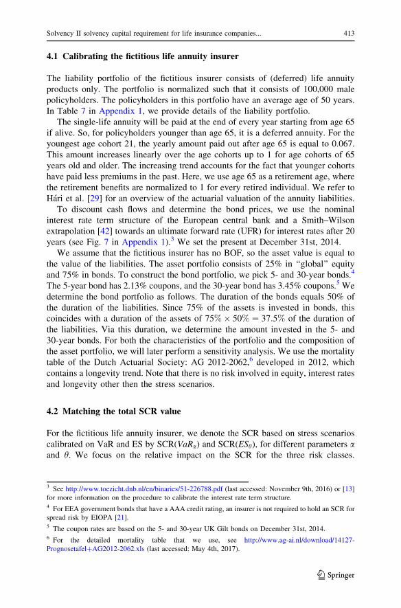
Figure 5 shows the change in allocation of the reduced total SCR for the three
different risk classes when ES is used to calibrate the shock scenarios instead of
VaR. The stress scenarios used to determine the SCR are this time determined
empirically. Similar as when EIOPA stress scenarios are used, the difference in
individual risk modules is small when a = 99.5%. Again, the differences are largest
when a is approximately 98.5%. At the quantile a ¼ 98:5%, the differences are
considerably larger compared to the base case, since the longevity SCR is
approximately 11:26% higher and the equity SCR is approximately 2:85% lower for
SCR(EShðaÞ) when compared with SCR(VaRa). For smaller values of the quantile auntil approximately 97.5% we see that the differences are getting smaller. The
changes in interest rate SCR differ substantially when empirical stress scenarios are
used compared to when EIOPA stress scenarios are used. For values of the quantile
a smaller than 97.5%, we see that the differences are stable, and differences in the
420 T. J. Boonen
123
interest rate SCR are smallest. We also see this in Fig. 4 in Sect. 5.1.1, where
EIOPA stress scenarios are used.
Comparing Figs. 4 and 5, we get that the differences in the SCR allocation when
ES is used instead of VaR are considerably larger when the stress scenarios are
calibrated empirically. The longevity SCR will increase more when ES is used
instead of VaR and when the quantile a is below 99%. This increase is at the
expense of a lower interest rate SCR.
For both using EIOPA stress scenarios and empirical stress scenarios we see that
the changes in allocation of the reduced total SCR are small for the quantile a ¼99:5% as used in solvency II. When the quantile a decreases, the differences
between the SCR allocation when ES is used instead of VaR get larger. We get that
by using ES to determine the shocks, longevity risk is more harmful and equity risk
is milder, particularly at the quantile a ¼ 98:5%. When we decrease the quantile auntil approximately 97.5%, these effects are getting smaller.
Table 5 Overview of the SCR changes of different risk classes using VaR99:5%, if we switch from PCA
analysis for interest shocks and the Gaussian approximations for longevity shocks to empirical interest
and longevity shocks
Change reduced total SCR 5:01%
Change interest rate SCR � 13:09%
Change equity SCR 0:00%
Change market SCR � 4:82%
Change longevity SCR 96:11%
All changes in SCR are expressed as percentage of the BEL
Fig. 5 Comparing the allocation of SCR(VaRa) with the allocation of SCR(EShðaÞ) for the fictitious life
annuity insurer, when the stress scenarios are determined empirically. The horizontal axis represents thequantile a used for VaR in the calibration method. The vertical axis represents the change in allocation ofthe SCRs when the stress scenarios are calibrated with ES instead of VaR
Solvency II solvency capital requirement for life insurance companies... 421
123
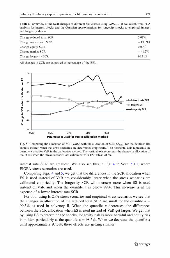
By comparing the empirical distribution of the tail of the data used for equity risk
and longevity risk we can explain why the differences are largest at approximately
98.5%. The downside tails of the data used for equity risk and longevity risk are
shown in Fig. 6. In this figure, both graphs have two horizontal axis. The first
horizontal axis represents the annual holding period return for equity risk and the
annual mortality rate changes for longevity risk. On the second horizontal axis, we
display the survival distribution (1—cumulative distribution).
One of the main characteristics of the VaR is that it does not consider the shape
of the tail. When the distribution has a heavy tail beyond the VaR level, then this
might lead to an underestimation of the risk. In Fig. 6, we see that the distribution of
longevity has a heavy tail and that the distribution of equity returns has a less heavy
tail. This explains why the longevity SCR is smaller and the equity SCR is larger if
we use VaR. To understand why the difference is largest for a � 98:5%, we focus
Fig. 6 The left tail (smallest 5%) of the empirical distribution for the data used in this paper for theequity returns (upper graph) and the mortality rate changes (lower graph). The first horizontal axisrepresents the annual holding period return of equity (upper graph) or the annual longevity changes(lower graph). For the second horizontal axis, we display the survival distribution (1—cumulativedistribution) of the empirical distribution. This helps us to determine the quantiles of the distribution. Thevertical axes represent the frequency
422 T. J. Boonen
123
on the empirical survival distribution. For equity risk the VaR98:5% is situated in the
middle of the heavy tail, therefore the equity SCR is relatively big when VaR is
used. For longevity risk, however, the VaR98:5% is situated just before the start of the
heavy tail, and this leads to a much smaller longevity SCR when VaR is used.
5.2 Sensitivity analysis
In this section, we study the sensitivity of our results. We do this by changing the
composition of the asset portfolio and the liability portfolio of the fictitious life
annuity insurer.
5.2.1 Changing the asset portfolio
As described in Sect. 4.1, the fictitious life annuity insurer has an asset portfolio
which consists of 25% in equity, and the remainder is invested in bonds. To test if
our results are sensitive to the composition of the asset portfolio we vary with the
percentage of equity in the portfolio and compare the allocation of SCR(VaRa) with
the allocation of SCR(EShðaÞ).
We analyze the following asset portfolios:
• 100% equity;
• 50% equity and 50% bonds;
• 25% equity and 75% bonds (base case);
• 10% equity and 90% bonds;
• 100% bonds.
When the asset portfolio contains bonds, the amounts invested in the 5- and 30-year
bonds are determined by matching the duration of the bond portfolio with 50% of
the duration of the liabilities. Hence, the duration is matched better when the insurer
invests more in bonds than in equity.
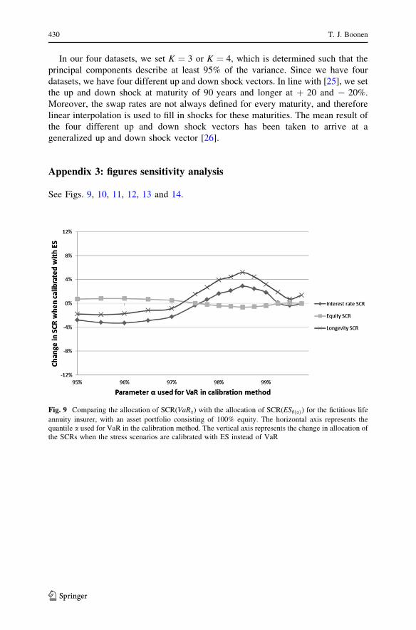
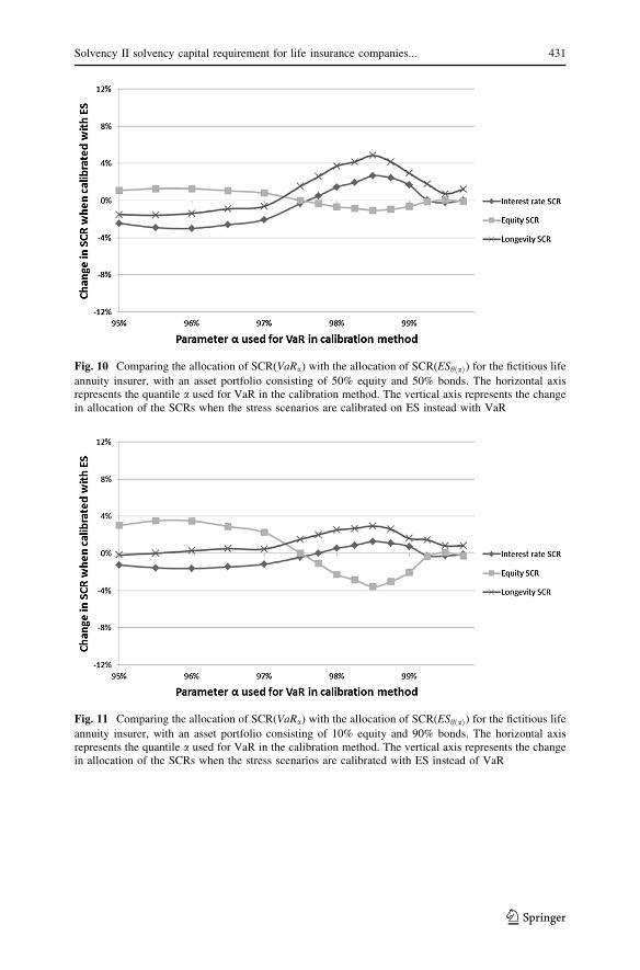
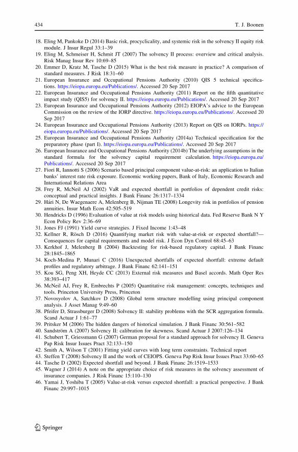
Figures 9, 10, 11 and 12 in Appendix 3 show the change in allocation of the
reduced total SCR for the three different risk classes when ES is used to calibrate
the shock scenarios instead of VaR for the different asset portfolios. To see how
sensitive our results are to the composition of the asset portfolio we can compare
these figures with Fig. 4.
When the equity holdings in the portfolio increase, we find a similar trend as in
the base case. The changes in allocation of the reduced total SCR are again small for
a ¼ 99:5%, i.e., using VaR or ES leads to similar stress scenarios for all three risk
classes. When the quantile a decreases, this difference becomes more significant and
is largest for a � 98:5%. For this quantile, the longevity SCR and the interest rate
SCR are larger and the equity SCR is smaller when the SCR is based on ES. When
we decrease the value a even more until 97.5%, the differences are getting smaller.
Figure 11 displays a similar trend as the base case, except for one difference. The
similarity with the base case is that the change in allocation of the reduced total SCR
is small for the quantile a ¼ 99:5%, is largest for the quantile a � 98:5%, and if we
decrease the quantile a until 97.5% the differences are getting smaller again. This
Solvency II solvency capital requirement for life insurance companies... 423
123
figure differs from the base case if we consider the percentage change in SCR per
risk class. When an asset portfolio of 10% equity and 90% bonds is used, the largest
percentage change is for the equity SCR. Whereas the relative change in equity SCR
grows in comparison with the base case, the change in longevity SCR and interest
rate SCR decreases in comparison with the base case. Overall, we still conclude that
the longevity SCR is larger and the equity SCR is smaller when ES is used.
Figure 12 looks somewhat different. In this case, the asset portfolio consists of
100% in bonds, so that there is no equity risk. We see however that the interest rate
SCR is smaller for all quantiles when ES is used.
From comparing Figs. 4, 10 and 11, we get that for different asset portfolios it
still holds that the differences in the SCR allocation are largest at a � 98:5% and
that the longevity SCR is larger and the equity SCR is smaller when ES is used. The
percentage change per risk class differs if the equity holdings change in the
portfolio, but the main trends remain similar.
5.2.2 Changing the liability portfolio
To test if our results are sensitive to the composition of the liability portfolio, we
vary with the distribution of the policyholders and compare the allocation of
SCR(VaRa) with the allocation of SCR(EShðaÞ). We show this comparison for the
following liability portfolios:
• young life annuity insurer: policyholders with an average age of 35;
• base case life annuity insurer: policyholders with an average age of 50;
• old life annuity insurer: policyholders with an average age of 65.
All other assumptions made in Sect. 4 still hold. For a precise description of the
liability portfolios, see Table 7 in Appendix 1. The number of policyholders per
liability portfolio is chosen based on matching the BEL to the BEL of the base case.
Similar to the base case, the asset portfolio consists of 25% in equity and 75% in
bonds. We again match 37:5% of the duration of the liabilities to determine the
amounts invested in the 5- and 30-year bonds.
We find that for the old life annuity insurer, the reduced total SCR is relatively
large compared to the BEL. The value of SCR(VaR99:5%) is 20.98% of the BEL,
compared to 23.24% for the baseline company. However, the longevity SCR for the
old company is 5.53%, and so larger than for the baseline company. The interest rate
SCR for the old company is however 6.42%, which is much smaller than 10.05% for
the baseline company. So, interest rate risk dominates the effect on the total SCR.
These findings for the young life annuity insurer are qualitatively similar.
Figures 13 and 14 in Appendix 3 show the change in allocation of the reduced
total SCR for the three different risk classes when ES is used to calibrate the shock
scenarios instead of VaR for the different liability portfolios. To see how sensitive
our results are to the composition of the liability portfolio we can compare Figs. 13
and 14 with Fig. 4. For all liability portfolios, the change in allocation of the
reduced total SCR is small when a ¼ 99:5%. This difference is largest for
a � 98:5%; for smaller a the differences are getting smaller until approximately
424 T. J. Boonen
123
97:5%. We observe that for all liability portfolios that the longevity SCR is larger
and the equity SCR is smaller when ES is used. For the value a ¼ 98:5%, it holds
for all three different liability portfolios that the longevity SCR increases with
approximately 4% and the equity SCR decreases with approximately 2:5% if ES
was used instead of VaR. If we compare Figs. 13 and 14 we get that relative interest
rate SCR changes are amplified for an older composition of the liability portfolio.
6 Other regulatory frameworks
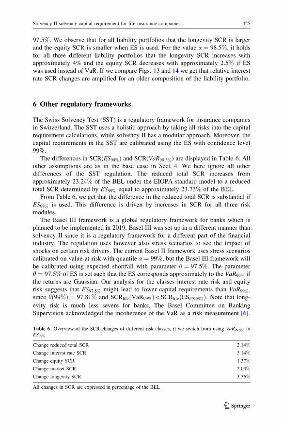
The Swiss Solvency Test (SST) is a regulatory framework for insurance companies
in Switzerland. The SST uses a holistic approach by taking all risks into the capital
requirement calculations, while solvency II has a modular approach. Moreover, the
capital requirements in the SST are calibrated using the ES with confidence level
99%.
The differences in SCR(ES99%) and SCR(VaR99:5%) are displayed in Table 6. All
other assumptions are as in the base case in Sect. 4. We here ignore all other
differences of the SST regulation. The reduced total SCR increases from
approximately 23:24% of the BEL under the EIOPA standard model to a reduced
total SCR determined by ES99% equal to approximately 23:73% of the BEL.
From Table 6, we get that the difference in the reduced total SCR is substantial if
ES99% is used. This difference is driven by increases in SCR for all three risk
modules.
The Basel III framework is a global regulatory framework for banks which is
planned to be implemented in 2019. Basel III was set up in a different manner than
solvency II since it is a regulatory framework for a different part of the financial
industry. The regulation uses however also stress scenarios to see the impact of
shocks on certain risk drivers. The current Basel II framework uses stress scenarios
calibrated on value-at-risk with quantile a ¼ 99%, but the Basel III framework will
be calibrated using expected shortfall with parameter h ¼ 97:5%. The parameter
h ¼ 97:5% of ES is set such that the ES corresponds approximately to the VaR99% if
the returns are Gaussian. Our analysis for the classes interest rate risk and equity
risk suggests that ES97:5% might lead to lower capital requirements than VaR99%,
since hð99%Þ ¼ 97:81% and SCRlifeðVaR99%Þ\SCRlifeðEShð99%ÞÞ. Note that long-
evity risk is much less severe for banks. The Basel Committee on Banking
Supervision acknowledged the incoherence of the VaR as a risk measurement [6].
Table 6 Overview of the SCR changes of different risk classes, if we switch from using VaR99:5% to
ES99%
Change reduced total SCR 2:14%
Change interest rate SCR 3:14%
Change equity SCR 1:37%
Change market SCR 2:03%
Change longevity SCR 3:36%
All changes in SCR are expressed in percentage of the BEL
Solvency II solvency capital requirement for life insurance companies... 425
123
7 Conclusion
This paper examines the consequences for a life annuity insurer if the solvency II
SCR calibration is based on expected shortfall (ES) instead of value-at-risk (VaR).
First, we calibrate the SCR stress scenarios for equity risk, interest rate risk and
longevity risk based on value-at-risk and expected shortfall. Thereafter, we compare
the SCR(VaRa) with the SCR(EShðaÞ) for a fictitious life annuity insurer.
Since we define hðaÞ such that SCR(VaRa) equals SCR(EShðaÞ), we focus on the
allocation of the reduced total SCR for the three risk classes: equity SCR, interest
rate SCR and longevity SCR. For the quantile a ¼ 99:5%, as used in solvency II, the
difference in allocation is small between SCR(VaRa) with the SCR(EShðaÞ), i.e., the
equity SCR, interest rate SCR and longevity SCR differ little is we use the VaR or
ES. Of course, this only applies if the confidence level hð99:5%Þ ¼ 98:78% is
applied for determining the expected shortfall. When a � 98:5%, the differences are
largest. If we use the ES instead of the VaR to determine the shocks, the longevity
SCR is larger and equity SCR is smaller. For smaller values of a, the differences
become smaller.
These results are robust in terms of variation with the composition of the asset
and liability portfolio of the life annuity insurer. To test the sensitivity of our results
to the calibration methods used by EIOPA, we compare the results with the SCR
allocations when the stress scenarios are determined empirically. We find that when
empirical stress scenarios are used, the reduced total SCR increases due to a higher
longevity SCR. Moreover, the interest rate SCR is smaller compared to when the
calibration methods are as determined by EIOPA [25].
Acknowledgements The author thanks Wouter Alblas for excellent research assistance. Preliminary
results of this article were based on his excellent MSc thesis at the University of Amsterdam under the
author’s supervision. Moreover, the author thanks Vali Asimit, Thomas Post and Sally Shen for valuable
comments. All remaining errors are the author’s responsibility.
Open Access This article is distributed under the terms of the Creative Commons Attribution 4.0
International License (http://creativecommons.org/licenses/by/4.0/), which permits unrestricted use, dis-
tribution, and reproduction in any medium, provided you give appropriate credit to the original
author(s) and the source, provide a link to the Creative Commons license, and indicate if changes were
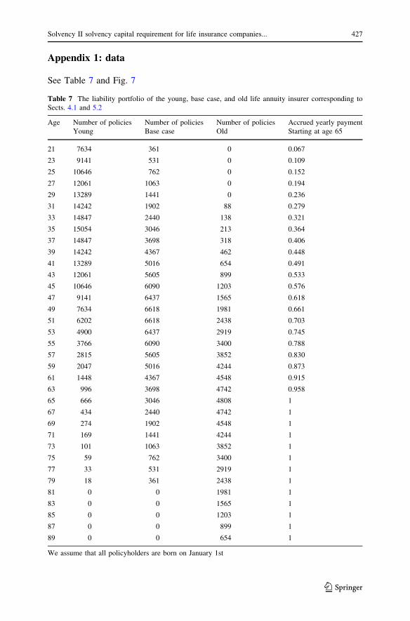
Table 7 The liability portfolio of the young, base case, and old life annuity insurer corresponding to
Sects. 4.1 and 5.2
Age Number of policies
Young
Number of policies
Base case
Number of policies
Old
Accrued yearly payment
Starting at age 65
21 7634 361 0 0.067
23 9141 531 0 0.109
25 10646 762 0 0.152
27 12061 1063 0 0.194
29 13289 1441 0 0.236
31 14242 1902 88 0.279
33 14847 2440 138 0.321
35 15054 3046 213 0.364
37 14847 3698 318 0.406
39 14242 4367 462 0.448
41 13289 5016 654 0.491
43 12061 5605 899 0.533
45 10646 6090 1203 0.576
47 9141 6437 1565 0.618
49 7634 6618 1981 0.661
51 6202 6618 2438 0.703
53 4900 6437 2919 0.745
55 3766 6090 3400 0.788
57 2815 5605 3852 0.830
59 2047 5016 4244 0.873
61 1448 4367 4548 0.915
63 996 3698 4742 0.958
65 666 3046 4808 1
67 434 2440 4742 1
69 274 1902 4548 1
71 169 1441 4244 1
73 101 1063 3852 1
75 59 762 3400 1
77 33 531 2919 1
79 18 361 2438 1
81 0 0 1981 1
83 0 0 1565 1
85 0 0 1203 1
87 0 0 899 1
89 0 0 654 1
We assume that all policyholders are born on January 1st
Solvency II solvency capital requirement for life insurance companies... 427
123
Appendix 2: interest rate risk stress scenarios by using principalcomponent analysis
In this appendix, we describe the principal component analysis (PCA) to calibrate
the interest rate shocks. PCA is used to describe movements of the yield curve and is
explained by Fiori and Iannotti [27] and Barber and Copper [5]. It applies an
orthogonal linear transformation that converts interest rate changes data of
correlated variables into a set of values of linearly uncorrelated variables. For the
m maturities, the relative yield curve change can then be represented exactly as a
linear combination of m vectors:
Xt ¼ ct þ b1;tU1 þ � � � þ bm;tUm ð13Þ
where Xt is the relative change in the annualized yield curve at time t ¼ 1; . . .; T , ctis a time-varying constant, and Uk are time-independent, zero-mean m� 1 vectors
that are orthogonal.
The data is then transformed into a new coordinate system such that the first
coordinate (i.e., the principal component b1;t) explains the largest share of the
variance by any projection of the data, the second coordinate has the second largest
explanation of the variance, etcetera. The objective of PCA is to determine a small
set of components that best explain the total variance of the data. The number of
components is then small K m, but with high explanatory power:
Xt ¼ ct þ b1;tU1 þ � � � þ bK;tUK þ et
where et is a zero-mean error term.
When PCA is used to describe interest rate movements, the factors Uk; k ¼1; . . .;K are the eigenvectors of the covariance matrix of the original data. The first
six components explain between 99.2 and 99.5% of the variance with a 90%
Fig. 7 The nominal interest rate term structure from the European Central Bank of December 31st, 2014,used in Sect. 4.3. Source: http://www.dnb.nl/statistiek/statistieken-dnb/index.jsp (last accessed: May 4th,2017)
confidence interval (cf. [5]). The principal components describe the different yield
curve movements and the first three are interpreted as the shift, twist and butterfly
moves of the yield curve [31, 37]. Figure 8 shows the first three eigenvectors of the
Euro vs Euribor IR swap rates. In this figure, we observe the shift, twist and butterfly
moves.
The principal components are derived via the following matrix multiplication:
bk;t ¼ U0kXt; for k ¼ 1; 2; . . .;K: ð14Þ
To transform the principal components and eigenvectors into VaR and ES based
interests rate stress scenarios, we use a method of Fiori and Iannotti [27]. For a
maturity k, we regress the relative annual percentage rate changes on the principal
components to derive the ‘‘beta’’ sensitivity of each rate to each principal compo-
nent via (14). We use the empirical distribution of each principal component vector
bk. Via historical simulation of the principal components, we derive a down risk
stress scenario and an up risk stress scenario for both VaR and ES as follows:
VaRc ¼ VaRc
XKk¼1
bkUk
!; for c ¼ a; ð1� aÞ; ð15Þ
ESc ¼ EScXKk¼1
bkUk
!; for c ¼ hðaÞ; 1� hðaÞ: ð16Þ
Since the eigenvectors Uk; k ¼ 1; . . .;K are orthogonal, we can randomly draw the
marginal distributions of bk; k ¼ 1; . . .;K and determine the empirical distribution
ofPK
k¼1 bkUk accordingly (see, e.g., [27]). We use 4000 simulations for each
dataset.
Fig. 8 The shift (PC1), twist (PC2) and butterfly (PC3) components of the yield curve of the Euro vsEuribor IR swap rates. The horizontal axis represents the term to maturity and the vertical axis representsthe level of the eigenvector component
Solvency II solvency capital requirement for life insurance companies... 429
123
In our four datasets, we set K ¼ 3 or K ¼ 4, which is determined such that the
principal components describe at least 95% of the variance. Since we have four
datasets, we have four different up and down shock vectors. In line with [25], we set
the up and down shock at maturity of 90 years and longer at þ 20 and - 20%.
Moreover, the swap rates are not always defined for every maturity, and therefore
linear interpolation is used to fill in shocks for these maturities. The mean result of
the four different up and down shock vectors has been taken to arrive at a
generalized up and down shock vector [26].
Appendix 3: figures sensitivity analysis
See Figs. 9, 10, 11, 12, 13 and 14.
Fig. 9 Comparing the allocation of SCR(VaRa) with the allocation of SCR(EShðaÞ) for the fictitious life
annuity insurer, with an asset portfolio consisting of 100% equity. The horizontal axis represents thequantile a used for VaR in the calibration method. The vertical axis represents the change in allocation ofthe SCRs when the stress scenarios are calibrated with ES instead of VaR
430 T. J. Boonen
123
Fig. 10 Comparing the allocation of SCR(VaRa) with the allocation of SCR(EShðaÞ) for the fictitious life
annuity insurer, with an asset portfolio consisting of 50% equity and 50% bonds. The horizontal axisrepresents the quantile a used for VaR in the calibration method. The vertical axis represents the changein allocation of the SCRs when the stress scenarios are calibrated on ES instead with VaR
Fig. 11 Comparing the allocation of SCR(VaRa) with the allocation of SCR(EShðaÞ) for the fictitious life
annuity insurer, with an asset portfolio consisting of 10% equity and 90% bonds. The horizontal axisrepresents the quantile a used for VaR in the calibration method. The vertical axis represents the changein allocation of the SCRs when the stress scenarios are calibrated with ES instead of VaR
Solvency II solvency capital requirement for life insurance companies... 431
123
Fig. 12 Comparing the allocation of SCR(VaRa) with the allocation of SCR(EShðaÞ) for the fictitious life
annuity insurer, with an asset portfolio consisting of 100% bonds. The horizontal axis represents thequantile a used for VaR in the calibration method. The vertical axis represents the change in allocation ofthe SCRs when the stress scenarios are calibrated with ES instead of VaR
Fig. 13 Comparing the allocation of SCR(VaRa) with the allocation of SCR(EShðaÞ) for the young life
annuity insurer. The horizontal axis represents the quantile a used for VaR in the calibration method. Thevertical axis represents the change in allocation of the SCRs when the stress scenarios are calibrated withES instead of VaR
432 T. J. Boonen
123
References
1. Acerbi C (2002) Spectral measures of risk: a coherent representation of subjective risk aversion.
14. Cont R (2001) Empirical properties of asset returns: stylized facts and statistical issues. Quant Financ
1:223–236
15. Coppola M, D’Amato V (2014) Further results about calibration of longevity risk for the insurance
business. Appl Math 5:653–657
16. Danielsson J, Jorgensen BN, Samorodnitsky G, Sarma M, De Vries CG (2013) Fat tails, VaR and
subadditivity. J Econom 172:283–291
17. Doff R (2008) A critical analysis of the solvency II proposals. Geneva Pap Risk Insur Issues Pract
33:193–206
Fig. 14 Comparing the allocation of SCR(VaRa) with the allocation of SCR(EShðaÞ) for the old life
annuity insurer. The horizontal axis represents the quantile a used for VaR in the calibration method. Thevertical axis represents the change in allocation of the SCRs when the stress scenarios are calibrated withES instead of VaR
Solvency II solvency capital requirement for life insurance companies... 433