Solvent effects and more (Part I): Continuum models G´ erald MONARD Th´ eorie - Mod´ eliation - Simulation UMR 7565 CNRS - Universit´ e de Lorraine Facult´ e des Sciences - B.P. 239 54506 Vandœuvre-les-Nancy Cedex - FRANCE http://www.monard.info/
Transcript
Solvent effects and more (Part I):Continuum models
Faculte des Sciences - B.P. 23954506 Vandœuvre-les-Nancy Cedex - FRANCE
http://www.monard.info/
Outline1. Introduction to solvent effects
2. The QM scaling problem
3. The implicit solvent model
4. Models baseds on multipole expansion
5. The Self-Consistent Reaction Field (SCRF)
Introduction to solvent effects
Solvation (IUPAC)Any stabilizing interaction of a solute (or solute moiety) and the solvent[. . . ]. Such interactions generally involve electrostatic forces and van derWaals forces, as well as chemically more specific effects such as hydrogenbond formation.
How to model solvent effects when solute can besmall . . . or large ?
Two kinds of solvent effectsShort range
â e.g. hydrogen bonds, molecular reorientation in the presence of ions,etc .
â Specific solvation mainly concentrated in the first solvation shells.
â Must be described by explicit solvent molecules.
Long range
â or ”macroscopic”, it involves the screening of charges(solvent polarization).
â The long range part is responsible for generating a (macroscopic)dielectric constant different from 1.
â Can be described through the use of a dielectric continuum (implicitinteraction).
â The dielectric continuum only accounts for averaged solvent effects.
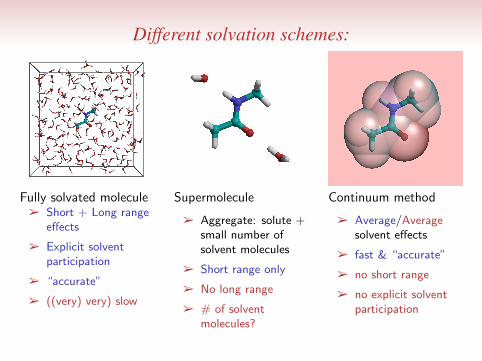
Different solvation schemes:
Fully solvated moleculeâ Short + Long range
effects
â Explicit solventparticipation
â “accurate”
â ((very) very) slow
Supermolecule
â Aggregate: solute +small number ofsolvent molecules
â Short range only
â No long range
â # of solventmolecules?
Continuum method
â Average/Averagesolvent effects
â fast & “accurate”
â no short range
â no explicit solventparticipation
The QM scaling problem
0
500
1000
1500
2000
2500
3000
3500
0 50 100 150 200
wall
clo
ck C
PU
tim
e (
seconds)
number of water molecules
energy of a water cluster (3-21G basis set)
B3LYP/3-21GBLYP/3-21G
CCSD(T)/3-21GMP2/3-21G
HF/3-21G
â (H2O)n water cluster(n from 1 to 216)
â 1 energy calculations
â Gaussian G09.B01(NProcShared=4, Mem=8Gb,MaxDisk=36Gb)
â Wall clock time limit: 1 hour
â Intel(R) Xeon(R) CPU E56202.40GHz (8 cores) 32Gb RAM
0
500
1000
1500
2000
2500
3000
3500
0 50 100 150 200
wall
clo
ck C
PU
tim
e (
seconds)
number of water molecules
energy of a water cluster (6-31G* basis set)
B3LYP/6-31G*BLYP/6-31G*
CCSD(T)/6-31G*MP2/6-31G*
HF/6-31G*
0
500
1000
1500
2000
2500
3000
3500
0 50 100 150 200
wall
clo
ck C
PU
tim
e (
seconds)
number of water molecules
energy of a water cluster (6-311+G** basis set)
B3LYP/6-311+G**BLYP/6-311+G**
CCSD(T)/6-311+G**MP2/6-311+G**
HF/6-311+G**
Quantum Chemistry is CPU intensive
Theoretical CPU scaling order for different QM methods
QM method Scaling
semiempirical O(N3)
DFT O(N3)
ab initio O(N4)
MP2 O(N5)
Full CI O(expN)
The (H2O)n example: n max in 1/2 hour (4 cores)
HF BLYP B3LYP MP2 CCSD(T)
3-21G 216 128 128 32 8
6-31G* 96 96 96 24 4
6-311+G** 32 32 28 16 4
How to solve the QM scaling problem?â Moore’s Law: CPU power doubles every 18 months
+ doubling a molecular system is possible:
3 O(N3) scaling: every 18x3 months = 4.5 years3 O(N4) scaling: every 6 years3 O(N5) scaling: every 7.5 years, etc.
â Parallelism is not a valid option in the long run
3 Good speeds-up are difficult to obtain (Amdahl’s Law)3 non linear scaling of the “standard” algorithms
+ limit the number of atoms: use continuum models
+ change the methods: use approximate quantum methods
Thermodynamic Backgroundâ The Solvation free energy ∆Gsol is the free energy change to
transfer a molecule from vacuum to solvent.
â It can be approximated by:
∆Gsol = ∆Gcav + ∆Gvdw + ∆Gelec
â ∆Gcav is the free energy required to form the solute cavity (> 0);
â ∆Gvdw is the van der Waals interaction between the solute and thesolvent (mainly a dispersive term, < 0);
+ ∆Gcav + ∆Gvdw : steric or non-electrostatic contributions
â ∆Gelec is the electrostatic component.
∆Gsol
Continuum models differ by
â How the size and shape of the cavity is defined(spherical, ellipsoıdal, molecular, etc)
â How the dispersion contributions are calculated
â How the charge distribution of M is represented(multipole expansions, apparent surface charges, etc)
â How the solute is described (QM or MM)
â How the dielectric medium is described
Cavitation energy
The cavity can have different shapes
â Spherical
â Ellipsoıdal
â Molecular: e.g. van der Waals surface, solvent accessible surface(SAS), isodensity surface
Cavitation energy
Experimental fact
â ∆Gcav + ∆Gdis change proportionnaly to the surface area
∆Gcav + ∆Gdis =atoms
∑i
ξiSi
â where ξi are an empirical atomic parameters, and Si are fractionalcontributions to the SAS by atoms i
â Continuum solvation models mainly differs by the way they calculate∆Gelec
The Classical Electrostatic Modelâ Poisson(-Boltzmann) equation:
−ε(r)∇2Φ(r) = 4πρ(r)
ε(r) = 1 for r ∈ Vin (inside the cavity)ε(r) = εs for r ∈ Vout (outside the cavity)ρ(r) = 0 for r ∈ Vout (charge distribution confined in the cavity)Φ(r) the total electrostatic potential
â ∆Gelec is obtained from two independent calculations:
∆Gelec =1
2
∫r∈Vin
ρ(r)[Φsol (r)−Φ0(r)
]Φsol (r) ε = 1 in Vin ε = εs in Vout
Φ0(r) ε = 1 in Vin ε = 1 in Vout
Some Models Based on Multipole Expansion
The Born Model (1920)A charge q inside a spherical cavity of radius a
∆Gelec =−1
2
(1− 1
εs
)q2
a
a the radius of the cavityq the point charge at the center of the cavity
Some Models Based on Multipole Expansion
The Kirkwood Model (1934)
â Generalization to a discrete charge distribution
∆Gelec =−1
2
∞
∑l=0
l
∑m=−l
(1 + l)(εs −1)
(1 + l)εs + 1
(Mml )2
a2l+1
â where Mml is the m component of the multipolar moment of order l
describing the charge distribution, and calculated at the center ofthe spherical cavity.
Some Models Based on Multipole Expansion
The Onsager Model (1936)A dipole moment µ inside a spherical cavity of radius a
∆Gelec =− εs −1
2εs + 1
µ2
a3
(1− εs −1
2εs + 1
2α
a3
)−1
µ the dipole momentα the isotropic dipolar polarizability
Some Models Based on Multipole Expansion
The Generalized Born Approximation (1956 & 1990)
∆Gelec =−1
2
(1− 1
εs
) N
∑i
N
∑j
qiqjfGB
where
fBG =√r2ij + αiαje
−Dij
and
Dij =r2ij
4αiαj
αi : effective radii of atom i
+ SMx models (Cramer & Truhlar) + various MM implementation
Some Models Based on Multipole Expansion
The MPE Model: Rivail et al. (1973)
â MPE: MultiPole Expansion
â Generalization of the Kirkwood model to a quantum wavefunction
∆Gelec =−1
2
∞
∑l=0
l
∑m=−l
∞
∑l ′=0
l ′
∑m′=−l ′
Mml f mm′
ll ′ Mm′l ′
â Mml : components of the charge distribution (multicentered)
â f mm′ll ′ : reaction field factors
they depend only on the shape of the cavity and the dielectricconstant of the solvent.
The Self-Consistent Reaction Field (SCRF)When the solute is polarizable (e.g., when using a QM method):
â The solute charge distribution polarizes the solvent
â A charge surface density is induced along the surface of the cavity:
σ(rs) =(εs −1)
4π
~∇Φout(rs).n(rs) =(εs −1)
4πεs
~∇Φin(rs).n(rs)
rs : a point of the surface of the cavityn(rs): the normal vector to the cavity surface on that point
â This charge surface density polarizes back the solute
â Which in turn polarizes the solvent, etc .
â Self-converging process: the Self-Consistent Reaction Field (SCRF)
The Self-Consistent Reaction Field (SCRF)â Spherical and ellipsoidal cavities −→ analytical solutions
â Molecular shaped cavities −→ numerical solutions
â Perturbation of the molecular hamiltonian:
H = H0 +Vσ
Vσ (r) =∫
σ(rs)
|r− rs |drs
â Iterative procedure + included in the SCF
â Many implementation: PCM (Polarizable Continuum Model),COSMO, . . .
Some SCRF Models in Quantum Chemistry
The PCM Model: Tomasi et al. (1981)
â PCM: Polarizable Continuum Model
â The surface of the cavity is divided into tesserae, each with an area∆Sk containing a charge qk
â Point charges on the cavity surface:
qk =−σ(rk)∆Sk
â qk charges are incorporated into the core hamiltonian
Vσ (r) = ∑k
qk|r− rk |
â Different cavity shapes can be used
Selected Reviewsâ Tomasi, J. and Persico, M., Chem. Rev., 1994, 94, 2027–2094;
Tomasi, J.; Mennucci, B. and Cammi, R., Chem. Rev., 2005, 105,2999–3093
â Cramer, C. J. and Truhlar, D. G., Acc. Chem. Res., 2008, 41(6),760–768;
Klamt, A.; Mennucci, B.; Tomasi, J.; Barone, V.; Curutchet, C.;Orozco, M. and Luque, F. J., Acc. Chem. Res., 2009, 42(4), 489–92;
Cramer, C. J. and Truhlar, D. G., Acc. Chem. Res., 2009, 42(4),493–497
â Monard, G. and Rivail, J.-L., In Handbook of ComputationalChemistry, Leszczynski, J., 2012
Some Illustrative ExamplesCurutchet, C.; Cramer, C. J.; Truhlar, D. G.; Ruiz-Lopez, M. F.; Rinaldi, D.;Orozco, M. and Luque, F. J., J. Comput. Chem., 2003, 24, 284–297Comparison of SCRF Continuum Models
â PCM and MPE behaves quite identically
â Predicted solvation free energies < 0.5kcal/mol compared toexperiment
Cappelli, C.; Corni, S. and Tomasi, J., J. Phys. Chem. A, 2001, 105(48),10807–10815Solvent effects on trans/gauche conformational equilibria of substitutedchloroethanes
Abul Kashem Liton, M.; Idrish Ali, M. and Tanvir Hossain, M., Comput.Theor. Chem., 2012, 999, 1–6pKa calculations for trimethylaminium ion