Universidade Nova de LisboaFaculdade de Ciências e Tecnologia

Departamento de Informática

Dissertação de Mestrado

Mestrado em Engenharia Informática

Solving Colored Nonograms

Luís Pedro Canas Ferreira Mingote(aluno nº 29634)

2º Semestre de 2008/0929 de Julho de 2009

Universidade Nova de LisboaFaculdade de Ciências e Tecnologia

Departamento de Informática

Dissertação de Mestrado

Solving Colored Nonograms

Luís Pedro Canas Ferreira Mingote(aluno nº 29634)

Orientador: Prof. Doutor Francisco de Azevedo

Trabalho apresentado no âmbito do Mestrado em Engen-haria Informática, como requisito parcial para obtenção dograu de Mestre em Engenharia Informática.

2º Semestre de 2008/0929 de Julho de 2009

Acknowledgements

In advance, I would like to thank my wife Marta and my daughters Margarida and Matilefor all their support and patience during the time I spent with this work.

I also would like to thank Prof. Francisco de Azevedo for his time and orientation. I cannotthank him enough for all the patience in reading, understanding and proposing improvementsto my writings.

I also would like to thank Prof. Paula Amaral, from the Mathematics Department, for mak-ing available CPLEX for testing.

I would also like to thank all my family for their support.

v

Resumo

Nesta dissertação aprofundamos o estudo da resolução de nonogramas coloridos utilizandoProgramação Linear Inteira (PLI). As formas conhecidas de resolução deste tipo de problemassão a força-bruta, o método iterativo e PLI.

A nossa aproximação generaliza a utilizada por Robert A. Bosch desenvolvida para, apenas,nonogramas a preto e branco, tornando assim disponível uma solução nova e universal para aresolução de nonogramas utilizando PLI.

Sendo as implementações do método iterativo as que apresentam melhores resultados aonível do desempenho, desenvolvemos também um método híbrido que combina esta aproxi-mação e PLI.

Estes puzzles têm, muitas vezes, várias soluções. A forma de as encontrar pelo modo iter-ativo é uma pesquisa em árvore com retrocesso. De forma a encontrar as restantes soluções nanossa aproximação aplicamos um algoritmo que utiliza um corte binário para excluir soluçõesjá conhecidas.

Para efeito de testes comparativos entre as diversas aproximações ao problema, desenvolve-mos um gerador de nonogramas que permite definir a resolução do puzzle, o seu número decores e a densidade (número de células pintadas vs. resolução).

Finalmente comparamos o desempenho da nossa aproximação para resolver nonogramascoloridos com o da aproximação interativa.

Palavras-chave: Nonograma, pintar-por-números, PLI, Programação Linear Inteira

vii

Abstract

In this thesis we deepen the study of colored nonogram solving using Integer Linear Pro-gramming (ILP). The known methods for solving this kind of problems are the depth-first search(brute-force) one, the iterative one and the ILP one.

Our approach generalizes the one used by Robert A. Bosch which was developed for blackand white nonograms only, thus providing a new universal solution for solving nonograms usingILP.

Since the iterative implementations are the ones that present better performance results, wealso developed a hybrid method that combines this approach and the ILP one.

This puzzles often have more than one solution. The way to find them using the iterativemethod e to make a tree search with backtracking. In order to find the remaining solutions usingour approach, is to apply an algorithm that uses a binary cut to exclude already known solutions.

In order to perform comparative tests between approaches, we developed a nonogram gen-erator that allows us to define the resolution of the puzzle, its number of colors and its density(number of painted cell vs. resolution).

Finally we compare the performance of our approach in solving colored nonograms againstthe iterative one.

Keywords: Nonogram, paint-by-numbers, ILP, Integer Linear Programming

ix

Contents

1 Introduction 11.1 Context 11.2 Problem Description 1

1.2.1 Initial problems 11.2.2 Nonograms 1

1.2.2.1 Black and White Nonograms 21.2.2.2 Colored Nonograms 2

1.3 Scope of work and main contributions 31.4 Document structure 4

2 Nonograms 52.1 Black and white Nonograms 5

2.1.1 Simple boxes 62.1.2 Punctuating 72.1.3 Simple spaces 82.1.4 Mercury 92.1.5 Forcing 92.1.6 Glue 102.1.7 Joining and splitting 10

2.2 Colored Nonograms 112.2.1 Simple boxes 122.2.2 Punctuating 142.2.3 Simple spaces 142.2.4 Mercury 152.2.5 Forcing 162.2.6 Glue 162.2.7 Joining and splitting 17

2.3 Approaches to solving Nonograms 182.3.1 Depth-first search (brute-force) 192.3.2 Iterative approach 192.3.3 Integer Linear Programming approach 21

3 An ILP model for solving Colored Nonograms 233.1 Model Description 23

3.1.1 Notation 233.1.2 Variables 243.1.3 Block constraints 253.1.4 Double Coverage Constraints 26

xi

xii

3.1.5 Objective Function 283.1.6 Pre-conditions 28

3.2 Instantiation to Black and White Nonograms 293.3 Finding Multiple Solutions 293.4 Hybrid model 30

4 Results 334.1 Pure ILP approach 334.2 Nonogram Generator 344.3 Hybrid ILP approach 36

5 Conclusions and Future Work 39

A Full Results 41

B Nonogram File Formats 53B.1 Bosch based file format 53B.2 Olšák file format 58B.3 Hett based file format 59

List of Figures

1.1 Black and white nonogram example (unsolved: left, solved: right) 21.2 Colored Nonogram Example - "Fall" from [2] 3

2.1 Black and white nonogram example 62.2 Example for the method Simple boxes in black and white nonograms 72.3 Example for the method Punctuating 82.4 Example 1 for the method Simple spaces applied to a black and white nonogram 82.5 Example 2 for the method Simple spaces applied to a black and white nonogram 82.6 Example for the method Mercury 92.7 Example for the method Forcing 102.8 Example for the method Glue 102.9 Example for the method Joining and splitting applied to a black and white nono-

gram 112.10 Solving a black and white Nonogram Example 112.11 Solving a black and white Nonogram Example — after last (horizontal) iteration 122.12 Example 1 for the method Simple boxes 132.13 Example for the method Punctuating 142.14 Example 1 for the method Simple spaces 142.15 Example 2 for the method Simple spaces 152.16 Example for the method Mercury 152.17 Example for the method Forcing 162.18 Example for the method Glue 162.19 Example for the method Joining and splitting 172.20 Solving a Colored Nonogram Example — "Fall" from [2] 172.21 Solving a Colored Nonogram Example — "Fall" from [2] 182.22 Solving a Colored Nonogram Example — "Fall" from [2] — After final (hori-

zontal) iteration 192.23 Depth-first search — all possibilities for a line 20

4.1 Generated nonogram 35

xiii

List of Tables

2.1 Experimental Results (in seconds) 22

4.1 Experimental Results (in seconds) 334.2 Results of adding equation (4.1) to ILP (in seconds) 344.3 Number of solved puzzles by method and dimension 374.4 Number of solved puzzles by method and density 374.5 Average time to solve a puzzle by dimension 384.6 Average time to solve a puzzle by density 38

A.1 Full Results (in seconds) 42

xv

1 . Introduction

1.1 Context

The work hereby presented was developed during the Master Program in Computer Sci-ence Engineering (Bologna second cycle), under the original theme "Solving Problems fromCSPLib".

1.2 Problem Description

1.2.1 Initial problems

Initially, the purpose of this work was to solve problems from CSPLib (www.csplib.org), aknown library of problems for modeling and solving. Given the lack of knowledge about themajority of the existing problems and our interest in exploring and solving new problems, thusbroadening our knowledge base, we decided to analyze the following five:

• prob012: Nonograms

• prob020: Darts tournament

• prob022: Bus driver scheduling

• prob032: Maximum density still life

• prob037: Peg solitaire

Although some work was done on problem "prob032 - Maximum density still life", specifi-cally the implementation of the Bucket Elimination algorithm by [11], we decided to deepen thestudy about problem "prob012 - Nonograms" since it appeared to us that there were approachesthat had not been explorer, specially to what concerns colored nonograms.

1.2.2 Nonograms

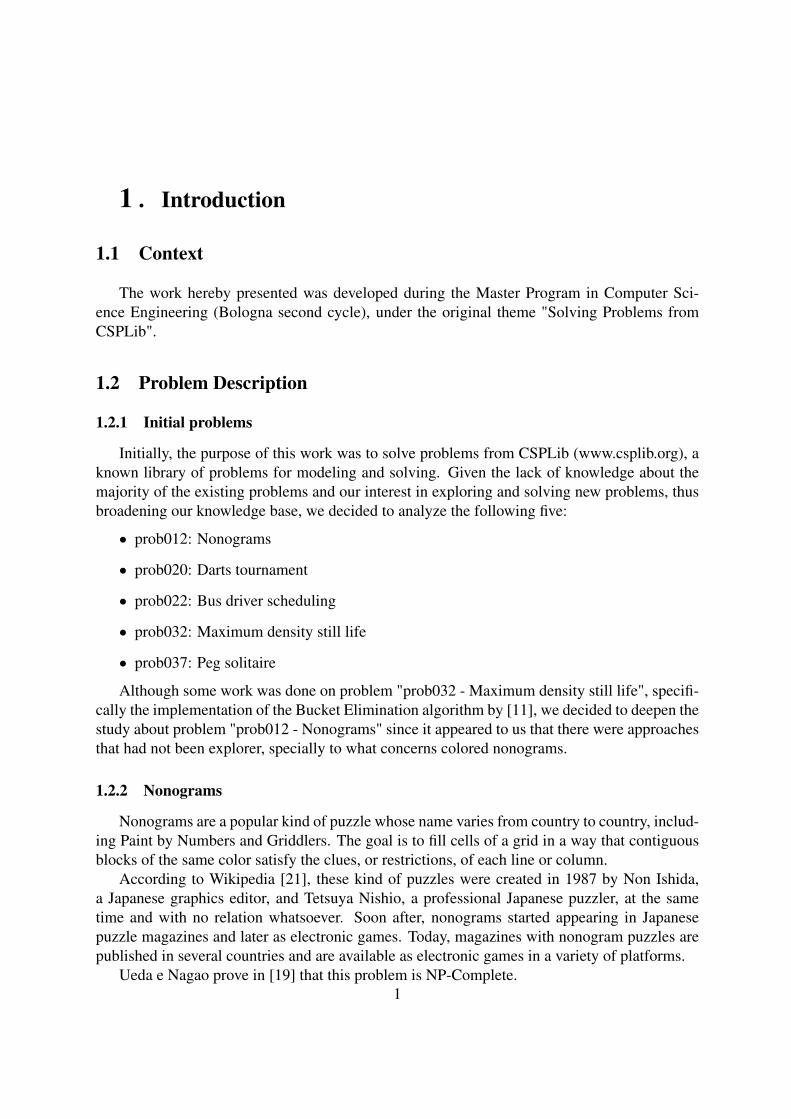
Nonograms are a popular kind of puzzle whose name varies from country to country, includ-ing Paint by Numbers and Griddlers. The goal is to fill cells of a grid in a way that contiguousblocks of the same color satisfy the clues, or restrictions, of each line or column.

According to Wikipedia [21], these kind of puzzles were created in 1987 by Non Ishida,a Japanese graphics editor, and Tetsuya Nishio, a professional Japanese puzzler, at the sametime and with no relation whatsoever. Soon after, nonograms started appearing in Japanesepuzzle magazines and later as electronic games. Today, magazines with nonogram puzzles arepublished in several countries and are available as electronic games in a variety of platforms.

Ueda e Nagao prove in [19] that this problem is NP-Complete.1

2

1.2.2.1 Black and White Nonograms

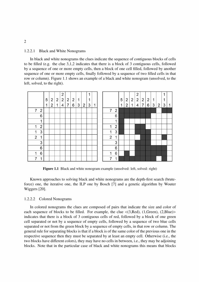
In black and white nonograms the clues indicate the sequence of contiguous blocks of cellsto be filled (e.g. the clue 3,1,2 indicates that there is a block of 3 contiguous cells, followedby a sequence of one or more empty cells, then a block of one cell filled, followed by anothersequence of one or more empty cells, finally followed by a sequence of two filled cells in thatrow or column). Figure 1.1 shows an example of a black and white nonogram (unsolved, to theleft, solved, to the right).

Figure 1.1 Black and white nonogram example (unsolved: left, solved: right)

Known approaches to solving black and white nonograms are the depth-first search (brute-force) one, the iterative one, the ILP one by Bosch [7] and a genetic algorithm by WouterWiggers [20].

1.2.2.2 Colored Nonograms

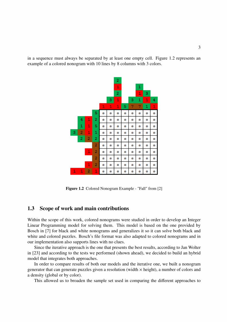
In colored nonograms the clues are composed of pairs that indicate the size and color ofeach sequence of blocks to be filled. For example, the clue <(3,Red), (1,Green), (2,Blue)>indicates that there is a block of 3 contiguous cells of red, followed by a block of one greencell separated or not by a sequence of empty cells, followed by a sequence of two blue cellsseparated or not from the green block by a sequence of empty cells, in that row or column. Thegeneral rule for separating blocks is that if a block is of the same color of the previous one in therespective sequence then they must be separated by at least an empty cell. Otherwise (i.e., thetwo blocks have different colors), they may have no cells in between, i.e., they may be adjoiningblocks. Note that in the particular case of black and white nonograms this means that blocks

3

in a sequence must always be separated by at least one empty cell. Figure 1.2 represents anexample of a colored nonogram with 10 lines by 8 columns with 3 colors.

Figure 1.2 Colored Nonogram Example - "Fall" from [2]

1.3 Scope of work and main contributions

Within the scope of this work, colored nonograms were studied in order to develop an IntegerLinear Programming model for solving them. This model is based on the one provided byBosch in [7] for black and white nonograms and generalizes it so it can solve both black andwhite and colored puzzles. Bosch’s file format was also adapted to colored nonograms and inour implementation also supports lines with no clues.

Since the iterative approach is the one that presents the best results, according to Jan Wolterin [23] and according to the tests we performed (shown ahead), we decided to build an hybridmodel that integrates both approaches.

In order to compare results of both our models and the iterative one, we built a nonogramgenerator that can generate puzzles given a resolution (width × height), a number of colors anda density (global or by color).

This allowed us to broaden the sample set used in comparing the different approaches to

4

solving nonograms thus providing a deeper comparison between them with tests over severalinstances of different dimensions and difficulty.

Our ILP approach was also enhanced in order to obtain more solutions to the same problem,if applicable. This enhancement was accomplished by simplifying a known algorithm that findsmultiple solutions in order to make it more efficient to this specific problem.

In summary, the main contributions of this work are:

• An ILP model for solving colored nonograms;

• A nonogram instance generator;

• An hybrid implementation between the iterative approach and our ILP approach for col-ored nonogram solving.

• A more systematic study of the different nonogram solving approaches

• An adaptation of an algorithm that obtains multiple solutions to an ILP problem, with asimplification that makes it more efficient to specific problems

1.4 Document structure

This document is organized in the following way: In Chapter 2 nonograms (both black andwhite and colored) are described in full and the best known approaches are detailed.

In Chapter 3 the ILP model we developed to solve colored nonograms is described, includ-ing a demonstration that this model corresponds to the one by Bosch in [7] for black and whitenonograms. It is also shown how to apply a simple technique in order to find additional solu-tions in case the first solution obtained for a puzzle is not unique. A description of the hybridapproach between the iterative approach and the hereby presented ILP model is also described.

In Chapter 4 results from the presented solutions are compared to its iterative counterpart.A description of the nonogram generator is also presented.

In Chapter 5 the results of the previous chapter are analyzed and the conclusions of thiswork are presented. We also suggest some future work based on the one presented here.

In appendix A a table with the result of all tests is show.in appendix B an example of each file format used is shown.

2 . Nonograms

In the previous chapter a brief description of nonograms was presented. In this one a moredetailed explanation about nonograms is shown.

Nonograms are a popular kind of puzzle whose name varies from country to country,including Paint by Numbers and Griddlers. The goal is to fill cells of a grid in a way thatcontiguous blocks of the same color satisfy the clues, or restrictions, of each line or column.

According to Wikipedia [21], these kind of puzzles were created in 1987 by Non Ishida,a Japanese graphics editor, and Tetsuya Nishio, a professional Japanese puzzler, at the sametime and with no relation whatsoever. Soon after, nonograms started appearing in Japanesepuzzle magazines and later as electronic games. Today, magazines with nonogram puzzles arepublished in several countries and are available as electronic games in a variety of platforms.

The most common nonograms are black and white, but they exist also in colors. In fact,black and white nonograms are a specialization of colored nonograms, i.e., are two colorednonograms.

Also there is a different kind of nonogram — called triddlers — in which cells are triangles.In this kind of puzzles we have three sets of clues instead of only two. These puzzles can alsoexist in multiple colors.

Ueda e Nagao prove in [19] that the nonogram problem is NP-Complete.

2.1 Black and white Nonograms

In black and white nonograms the clues indicate the sequence of contiguous blocks of cellsto be filled (e.g. the clue 3,1,2 indicates that there is a block of 3 contiguous cells, followedby a sequence of one or more empty cells, then a block of one cell filled, followed by anothersequence of one or more empty cells, finally followed by a sequence of two filled cells in thatrow or column). Figure 1.1 shows an example of a black and white nonogram (unsolved, to theleft, solved, to the right).

According to Wikipedia [21], in order to solve this kind of puzzle it is necessary todetermine which cells will be filled (black) and which will be empty (white). Determiningwhich cells will be empty is as important as determining which will be filled because the formerwill help delimiting the solutions for the blocks of each line or column1.

Simpler puzzles, like the one shown in figure 2.10, can usually be solved by applying thefollowing methods to each line at a time.

1For the sake of simplicity, from this point forward, only lines will be mentioned, since the reasoning is thesame for columns.

5

6

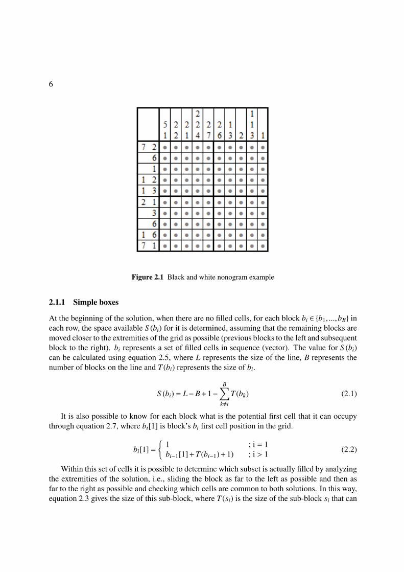
Figure 2.1 Black and white nonogram example

2.1.1 Simple boxes

At the beginning of the solution, when there are no filled cells, for each block bi ∈ {b1, ...,bB} ineach row, the space available S (bi) for it is determined, assuming that the remaining blocks aremoved closer to the extremities of the grid as possible (previous blocks to the left and subsequentblock to the right). bi represents a set of filled cells in sequence (vector). The value for S (bi)can be calculated using equation 2.5, where L represents the size of the line, B represents thenumber of blocks on the line and T (bi) represents the size of bi.

S (bi) = L−B+ 1−B∑

k,i

T (bk) (2.1)

It is also possible to know for each block what is the potential first cell that it can occupythrough equation 2.7, where bi[1] is block’s bi first cell position in the grid.

bi[1] =

{1 ; i = 1bi−1[1] + T (bi−1) + 1) ; i > 1 (2.2)

Within this set of cells it is possible to determine which subset is actually filled by analyzingthe extremities of the solution, i.e., sliding the block as far to the left as possible and then asfar to the right as possible and checking which cells are common to both solutions. In this way,equation 2.3 gives the size of this sub-block, where T (si) is the size of the sub-block si that can

7

be determined for block bi.

T (si) = 2T (bi)−S (bi) (2.3)

In the same way, it is possible to obtain the first cell (consequently the remaining) of thissub-block through equation 2.4, where si[1] is the position of the first cell of sub-block si.

si[1] = bi[1] + S (bi)−T (bi) ; T (si) > 0 (2.4)

Figure 2.2 Example for the method Simple boxes in black and white nonograms

As an example, for the 10th line of the puzzle shown in figure 2.1, L = 10, B = 2, T (b1) = 7and T (b2) = 1. Therefore the space available for the first block is S (b1) = 10− 2 + 1− 1 = 8and S (b2) = 10−2 + 1−7 = 2. The leftmost indexes each can occupy are b1[1] = 1 and b2[1] =

1 + 7 + 1 = 9.As for the sub-blocks of cells that can be filled at this point, T (s1) = 2× 7− 8 = 6 and

T (s2) = 2× 1− 2 = 0, i.e., it is not possible to fill, for now, any cell in respect to the secondblock, but it is possible to fill six cells with respect to the first one. It is yet to determine thestarting cell of the first and second sub-blocks: s1[1] = 1 + 8−7 = 2, i.e., it is possible to fill, atthis point, cells 2 through 7 of that line.

Figure 2.2, from line 10 of the puzzle shown in figure 2.1, exemplifies this method for a size10 line with with two blocks of sizes 7 and 1.

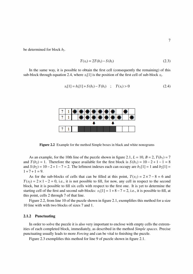
2.1.2 Punctuating

In order to solve the puzzle it is also very important to enclose with empty cells the extrem-ities of each completed block, immediately, as described in the method Simple spaces. Precisepunctuating usually leads to more Forcing and can be vital to finishing the puzzle.

Figure 2.3 exemplifies this method for line 9 of puzzle shown in figure 2.1.

8

Figure 2.3 Example for the method Punctuating

2.1.3 Simple spaces

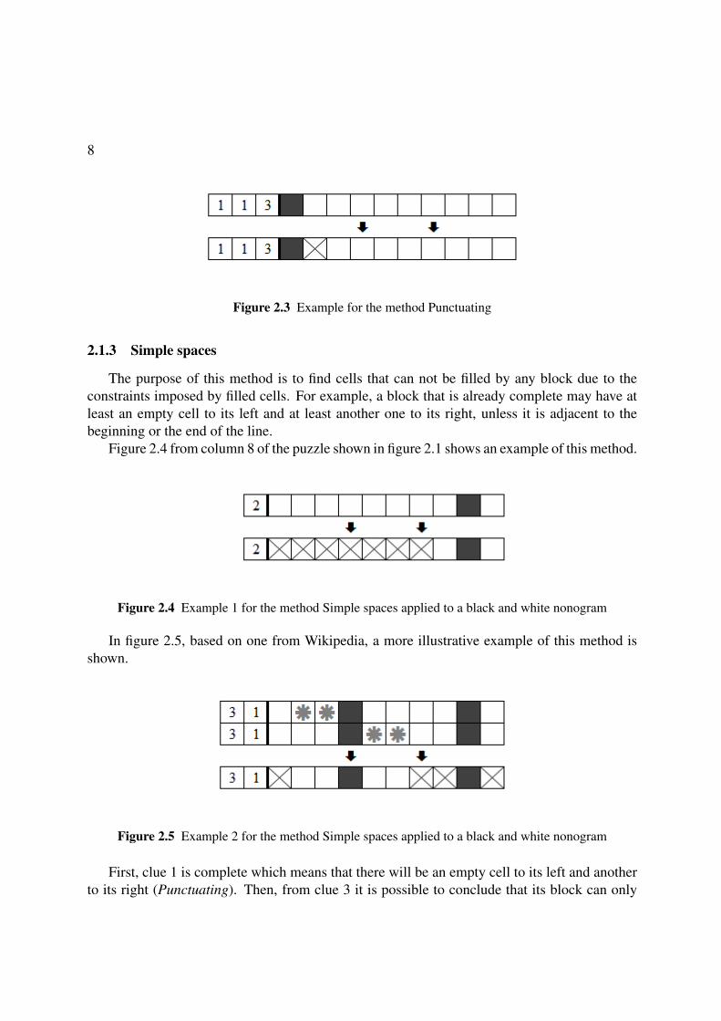
The purpose of this method is to find cells that can not be filled by any block due to theconstraints imposed by filled cells. For example, a block that is already complete may have atleast an empty cell to its left and at least another one to its right, unless it is adjacent to thebeginning or the end of the line.

Figure 2.4 from column 8 of the puzzle shown in figure 2.1 shows an example of this method.

Figure 2.4 Example 1 for the method Simple spaces applied to a black and white nonogram

In figure 2.5, based on one from Wikipedia, a more illustrative example of this method isshown.

Figure 2.5 Example 2 for the method Simple spaces applied to a black and white nonogram

First, clue 1 is complete which means that there will be an empty cell to its left and anotherto its right (Punctuating). Then, from clue 3 it is possible to conclude that its block can only

9

expand between the second and the sixth cell because it has to include the fourth cell. Thismeans that cells 1 and 7 will be empty.

2.1.4 Mercury

Mercury is a special case of Simple spaces. The name comes from the way mercury pulls backfrom the sides of a container.

If there is a filled cell on a line that is at the same distance from the border as the size of thefirst block, then the first cell has to be empty. This is true because the first block would not fitto the left of the filled cell. It will have to spread through that cell leaving the first cell behind.Besides, when the cell is in reality a set with cells more to the right, there will be more spacesat the beginning of the line, determined by applying this method several times.

In figure 2.6, from Wikipedia, an example of this method is shown.

Figure 2.6 Example for the method Mercury

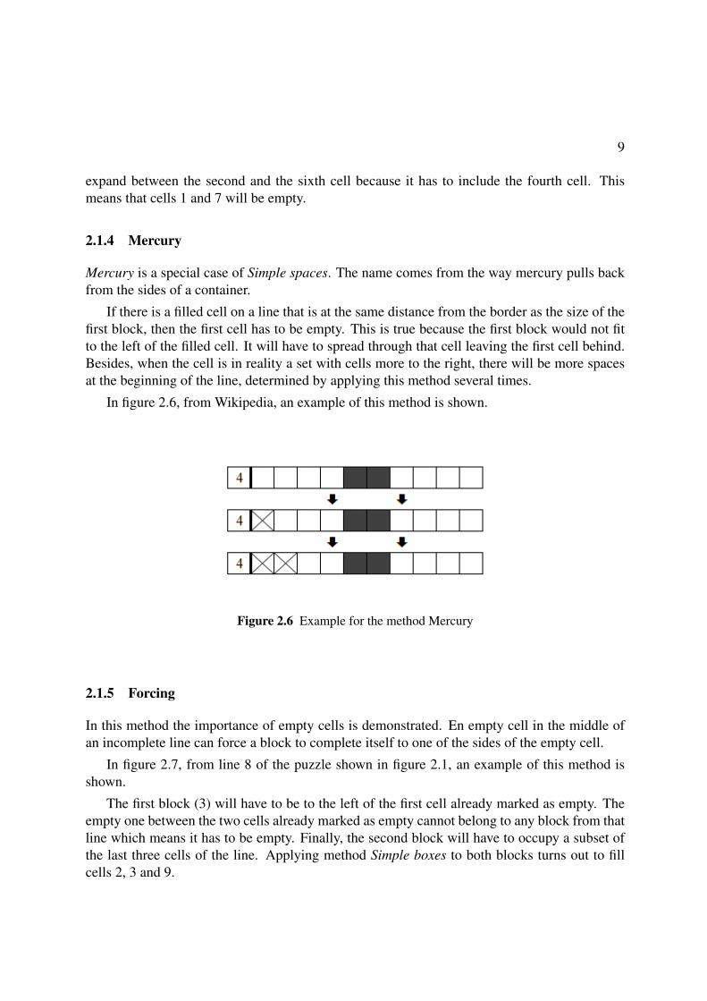
2.1.5 Forcing

In this method the importance of empty cells is demonstrated. En empty cell in the middle ofan incomplete line can force a block to complete itself to one of the sides of the empty cell.

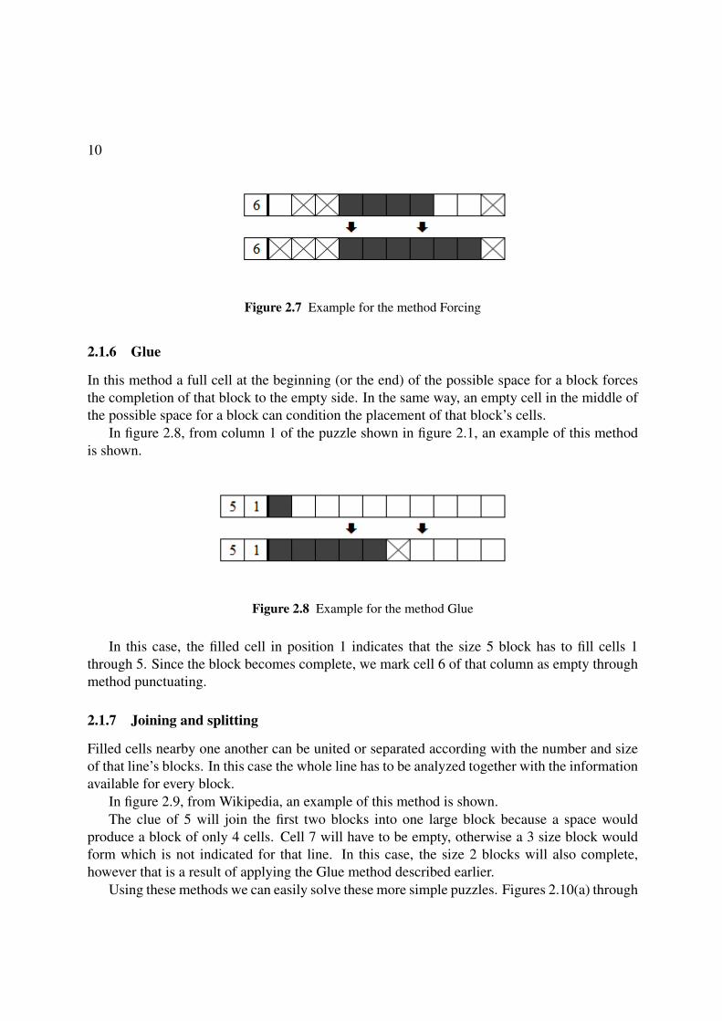
In figure 2.7, from line 8 of the puzzle shown in figure 2.1, an example of this method isshown.

The first block (3) will have to be to the left of the first cell already marked as empty. Theempty one between the two cells already marked as empty cannot belong to any block from thatline which means it has to be empty. Finally, the second block will have to occupy a subset ofthe last three cells of the line. Applying method Simple boxes to both blocks turns out to fillcells 2, 3 and 9.

10

Figure 2.7 Example for the method Forcing

2.1.6 Glue

In this method a full cell at the beginning (or the end) of the possible space for a block forcesthe completion of that block to the empty side. In the same way, an empty cell in the middle ofthe possible space for a block can condition the placement of that block’s cells.

In figure 2.8, from column 1 of the puzzle shown in figure 2.1, an example of this methodis shown.

Figure 2.8 Example for the method Glue

In this case, the filled cell in position 1 indicates that the size 5 block has to fill cells 1through 5. Since the block becomes complete, we mark cell 6 of that column as empty throughmethod punctuating.

2.1.7 Joining and splitting

Filled cells nearby one another can be united or separated according with the number and sizeof that line’s blocks. In this case the whole line has to be analyzed together with the informationavailable for every block.

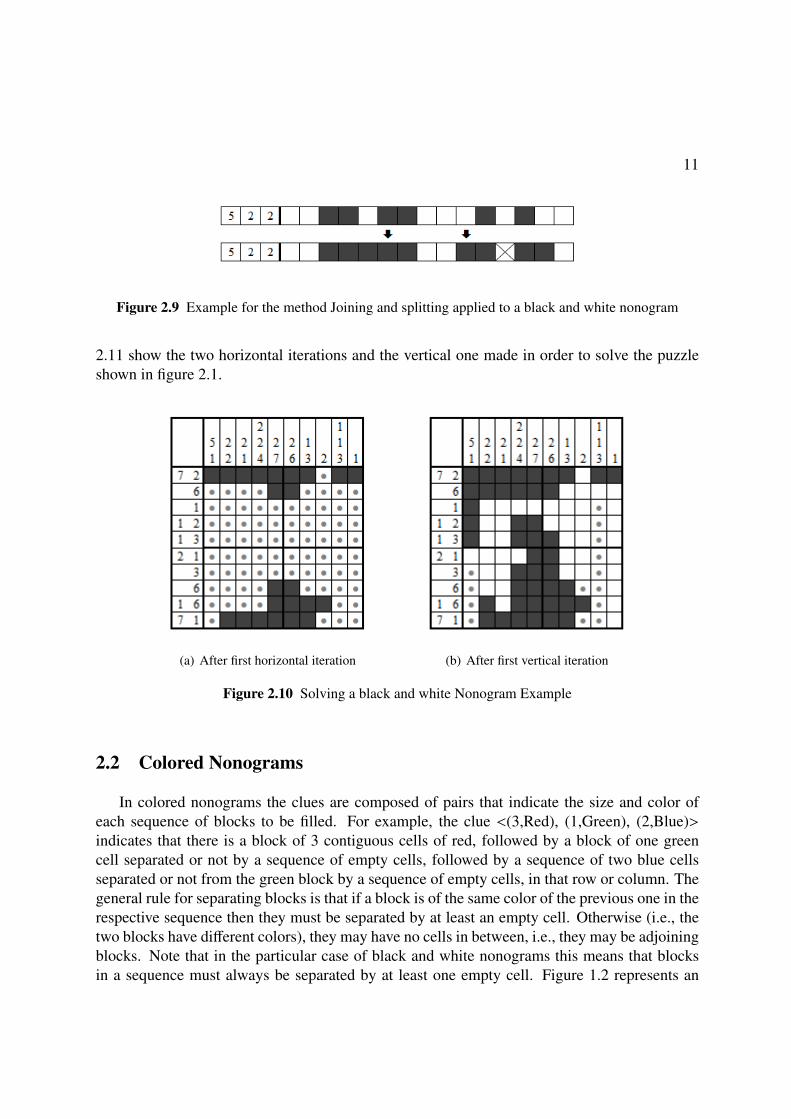
In figure 2.9, from Wikipedia, an example of this method is shown.The clue of 5 will join the first two blocks into one large block because a space would

produce a block of only 4 cells. Cell 7 will have to be empty, otherwise a 3 size block wouldform which is not indicated for that line. In this case, the size 2 blocks will also complete,however that is a result of applying the Glue method described earlier.

Using these methods we can easily solve these more simple puzzles. Figures 2.10(a) through

11

Figure 2.9 Example for the method Joining and splitting applied to a black and white nonogram

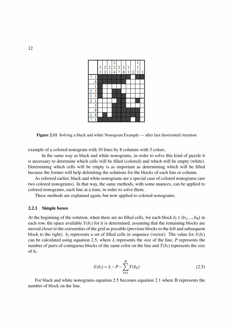
2.11 show the two horizontal iterations and the vertical one made in order to solve the puzzleshown in figure 2.1.

(a) After first horizontal iteration (b) After first vertical iteration

Figure 2.10 Solving a black and white Nonogram Example

2.2 Colored Nonograms

In colored nonograms the clues are composed of pairs that indicate the size and color ofeach sequence of blocks to be filled. For example, the clue <(3,Red), (1,Green), (2,Blue)>indicates that there is a block of 3 contiguous cells of red, followed by a block of one greencell separated or not by a sequence of empty cells, followed by a sequence of two blue cellsseparated or not from the green block by a sequence of empty cells, in that row or column. Thegeneral rule for separating blocks is that if a block is of the same color of the previous one in therespective sequence then they must be separated by at least an empty cell. Otherwise (i.e., thetwo blocks have different colors), they may have no cells in between, i.e., they may be adjoiningblocks. Note that in the particular case of black and white nonograms this means that blocksin a sequence must always be separated by at least one empty cell. Figure 1.2 represents an

12

Figure 2.11 Solving a black and white Nonogram Example — after last (horizontal) iteration

example of a colored nonogram with 10 lines by 8 columns with 3 colors.In the same way as black and white nonograms, in order to solve this kind of puzzle it

is necessary to determine which cells will be filled (colored) and which will be empty (white).Determining which cells will be empty is as important as determining which will be filledbecause the former will help delimiting the solutions for the blocks of each line or column.

As referred earlier, black and white nonograms are a special case of colored nonograms (aretwo colored nonograms). In that way, the same methods, with some nuances, can be applied tocolored nonograms, each line at a time, in order to solve them.

These methods are explained again, but now applied to colored nonograms.

2.2.1 Simple boxes

At the beginning of the solution, when there are no filled cells, for each block bi ∈ {b1, ...,bB} ineach row, the space available S (bi) for it is determined, assuming that the remaining blocks aremoved closer to the extremities of the grid as possible (previous blocks to the left and subsequentblock to the right). bi represents a set of filled cells in sequence (vector). The value for S (bi)can be calculated using equation 2.5, where L represents the size of the line, P represents thenumber of pairs of contiguous blocks of the same color on the line and T (bi) represents the sizeof bi.

S (bi) = L−P−B∑

k,i

T (bk) (2.5)

For black and white nonograms equation 2.5 becomes equation 2.1 where B represents thenumber of block on the line.

13

It is also possible to know for each block what is the potential first cell that it can occupythrough equation 2.7, where bi[1] is block’s bi first cell position in the grid and f is a functionthat returns 1 if the blocks are of the same color and 0 otherwise (see equation 2.6 where Cbi isthe color of block i).

f (bi,b j) =

{0 ; Cbi ,Cb j

1 ; Cbi = Cb j(2.6)

bi[1] =

{1 ; i = 1bi−1[1] + T (bi−1) + f (bi,bi−1) ; i > 1 (2.7)

For black and white nonograms f always returns 1 and equation 2.7 becomes equation 2.2.Within this set of cells it is possible to determine which subset is actually filled by analyzing

the extremities of the solution, i.e., sliding the block as far to the left as possible and then asfar to the right as possible and checking which cells are common to both solutions. In this way,equation 2.8 gives the size of this sub-block, where T (si) is the size of the sub-block si that canbe determined for block bi.

T (si) = 2T (bi)−S (bi) (2.8)

In the same way, it is possible to obtain the first cell (consequently the remaining) of thissub-block through equation 2.9, where si[1] is the position of the first cell of sub-block si.

si[1] = bi[1] + S (bi)−T (bi) ; T (si) > 0 (2.9)

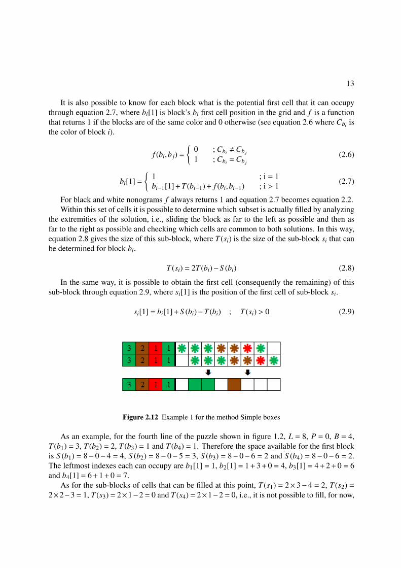
Figure 2.12 Example 1 for the method Simple boxes

As an example, for the fourth line of the puzzle shown in figure 1.2, L = 8, P = 0, B = 4,T (b1) = 3, T (b2) = 2, T (b3) = 1 and T (b4) = 1. Therefore the space available for the first blockis S (b1) = 8− 0− 4 = 4, S (b2) = 8− 0− 5 = 3, S (b3) = 8− 0− 6 = 2 and S (b4) = 8− 0− 6 = 2.The leftmost indexes each can occupy are b1[1] = 1, b2[1] = 1 + 3 + 0 = 4, b3[1] = 4 + 2 + 0 = 6and b4[1] = 6 + 1 + 0 = 7.

As for the sub-blocks of cells that can be filled at this point, T (s1) = 2× 3− 4 = 2, T (s2) =

2×2−3 = 1, T (s3) = 2×1−2 = 0 and T (s4) = 2×1−2 = 0, i.e., it is not possible to fill, for now,

14

any cell in respect to the third and fourth blocks, but it is possible to fill two cells with respectto the first one and one cell with respect to the second one. It is yet to determine the startingcell of the first and second sub-blocks: s1[1] = 1 + 4−3 = 2 and s2[1] = 4 + 3−2 = 5., i.e., it ispossible to fill, at this point, cells 2, 3 and 5 of that line.

2.2.2 Punctuating

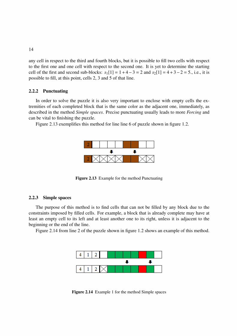
In order to solve the puzzle it is also very important to enclose with empty cells the ex-tremities of each completed block that is the same color as the adjacent one, immediately, asdescribed in the method Simple spaces. Precise punctuating usually leads to more Forcing andcan be vital to finishing the puzzle.

Figure 2.13 exemplifies this method for line line 6 of puzzle shown in figure 1.2.

Figure 2.13 Example for the method Punctuating

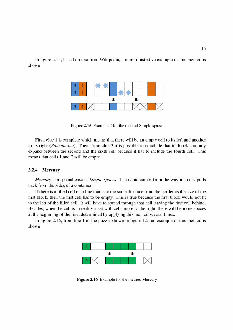
2.2.3 Simple spaces

The purpose of this method is to find cells that can not be filled by any block due to theconstraints imposed by filled cells. For example, a block that is already complete may have atleast an empty cell to its left and at least another one to its right, unless it is adjacent to thebeginning or the end of the line.

Figure 2.14 from line 2 of the puzzle shown in figure 1.2 shows an example of this method.

Figure 2.14 Example 1 for the method Simple spaces

15

In figure 2.15, based on one from Wikipedia, a more illustrative example of this method isshown.

Figure 2.15 Example 2 for the method Simple spaces

First, clue 1 is complete which means that there will be an empty cell to its left and anotherto its right (Punctuating). Then, from clue 3 it is possible to conclude that its block can onlyexpand between the second and the sixth cell because it has to include the fourth cell. Thismeans that cells 1 and 7 will be empty.

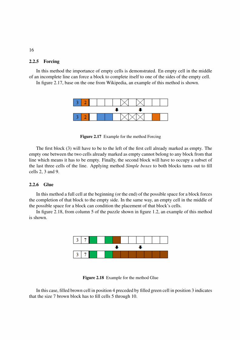
2.2.4 Mercury

Mercury is a special case of Simple spaces. The name comes from the way mercury pullsback from the sides of a container.

If there is a filled cell on a line that is at the same distance from the border as the size of thefirst block, then the first cell has to be empty. This is true because the first block would not fitto the left of the filled cell. It will have to spread through that cell leaving the first cell behind.Besides, when the cell is in reality a set with cells more to the right, there will be more spacesat the beginning of the line, determined by applying this method several times.

In figure 2.16, from line 1 of the puzzle shown in figure 1.2, an example of this method isshown.

Figure 2.16 Example for the method Mercury

16

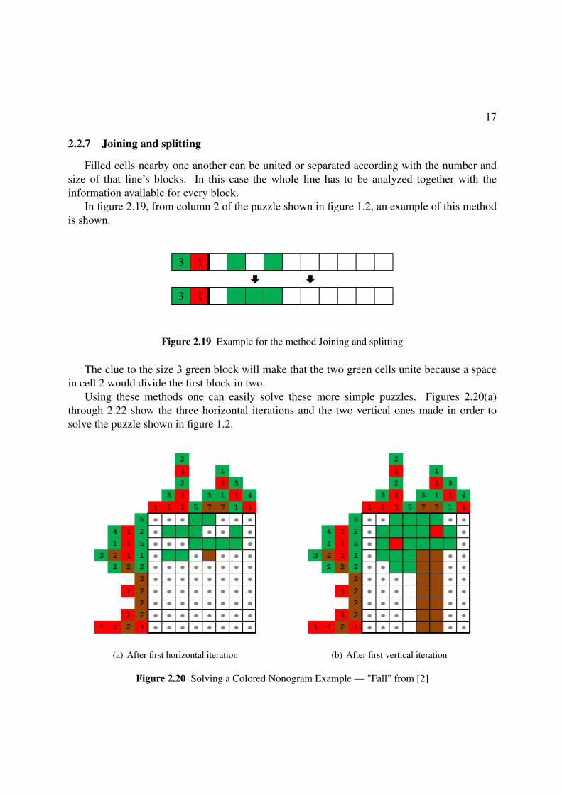
2.2.5 Forcing

In this method the importance of empty cells is demonstrated. En empty cell in the middleof an incomplete line can force a block to complete itself to one of the sides of the empty cell.

In figure 2.17, base on the one from Wikipedia, an example of this method is shown.

Figure 2.17 Example for the method Forcing

The first block (3) will have to be to the left of the first cell already marked as empty. Theempty one between the two cells already marked as empty cannot belong to any block from thatline which means it has to be empty. Finally, the second block will have to occupy a subset ofthe last three cells of the line. Applying method Simple boxes to both blocks turns out to fillcells 2, 3 and 9.

2.2.6 Glue

In this method a full cell at the beginning (or the end) of the possible space for a block forcesthe completion of that block to the empty side. In the same way, an empty cell in the middle ofthe possible space for a block can condition the placement of that block’s cells.

In figure 2.18, from column 5 of the puzzle shown in figure 1.2, an example of this methodis shown.

Figure 2.18 Example for the method Glue

In this case, filled brown cell in position 4 preceded by filled green cell in position 3 indicatesthat the size 7 brown block has to fill cells 5 through 10.

17

2.2.7 Joining and splitting

Filled cells nearby one another can be united or separated according with the number andsize of that line’s blocks. In this case the whole line has to be analyzed together with theinformation available for every block.

In figure 2.19, from column 2 of the puzzle shown in figure 1.2, an example of this methodis shown.

Figure 2.19 Example for the method Joining and splitting

The clue to the size 3 green block will make that the two green cells unite because a spacein cell 2 would divide the first block in two.

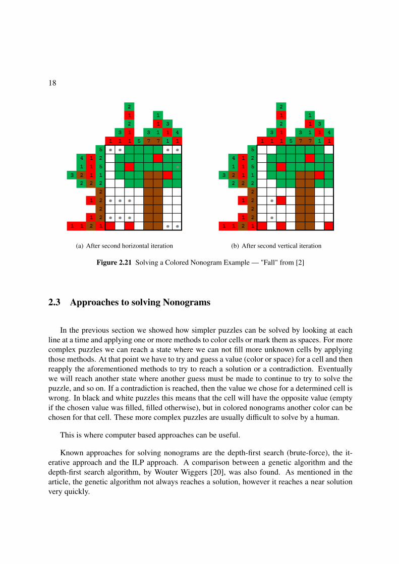
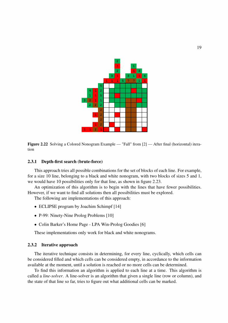
Using these methods one can easily solve these more simple puzzles. Figures 2.20(a)through 2.22 show the three horizontal iterations and the two vertical ones made in order tosolve the puzzle shown in figure 1.2.

(a) After first horizontal iteration (b) After first vertical iteration

Figure 2.20 Solving a Colored Nonogram Example — "Fall" from [2]

18

(a) After second horizontal iteration (b) After second vertical iteration

Figure 2.21 Solving a Colored Nonogram Example — "Fall" from [2]

2.3 Approaches to solving Nonograms

In the previous section we showed how simpler puzzles can be solved by looking at eachline at a time and applying one or more methods to color cells or mark them as spaces. For morecomplex puzzles we can reach a state where we can not fill more unknown cells by applyingthose methods. At that point we have to try and guess a value (color or space) for a cell and thenreapply the aforementioned methods to try to reach a solution or a contradiction. Eventuallywe will reach another state where another guess must be made to continue to try to solve thepuzzle, and so on. If a contradiction is reached, then the value we chose for a determined cell iswrong. In black and white puzzles this means that the cell will have the opposite value (emptyif the chosen value was filled, filled otherwise), but in colored nonograms another color can bechosen for that cell. These more complex puzzles are usually difficult to solve by a human.

This is where computer based approaches can be useful.

Known approaches for solving nonograms are the depth-first search (brute-force), the it-erative approach and the ILP approach. A comparison between a genetic algorithm and thedepth-first search algorithm, by Wouter Wiggers [20], was also found. As mentioned in thearticle, the genetic algorithm not always reaches a solution, however it reaches a near solutionvery quickly.

19

Figure 2.22 Solving a Colored Nonogram Example — "Fall" from [2] — After final (horizontal) itera-tion

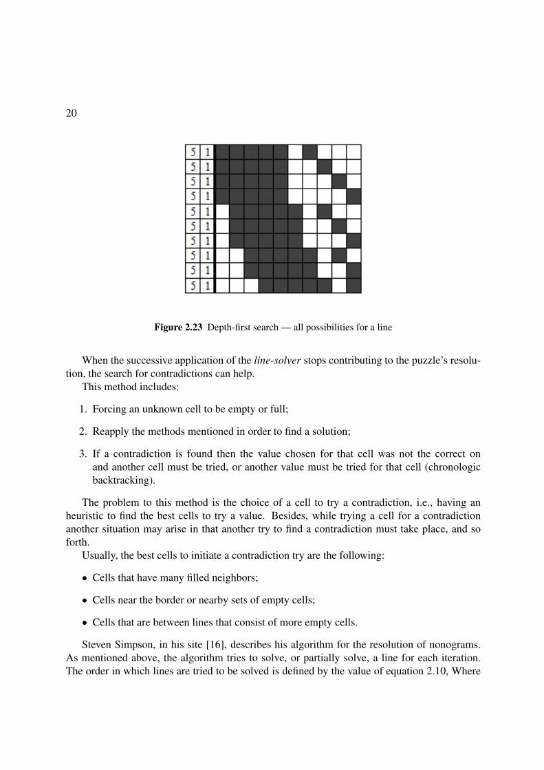
2.3.1 Depth-first search (brute-force)

This approach tries all possible combinations for the set of blocks of each line. For example,for a size 10 line, belonging to a black and white nonogram, with two blocks of sizes 5 and 1,we would have 10 possibilities only for that line, as shown in figure 2.23.

An optimization of this algorithm is to begin with the lines that have fewer possibilities.However, if we want to find all solutions then all possibilities must be explored.

The following are implementations of this approach:

• ECLIPSE program by Joachim Schimpf [14]

• P-99: Ninety-Nine Prolog Problems [10]

• Colin Barker’s Home Page - LPA Win-Prolog Goodies [6]

These implementations only work for black and white nonograms.

2.3.2 Iterative approach

The iterative technique consists in determining, for every line, cyclically, which cells canbe considered filled and which cells can be considered empty, in accordance to the informationavailable at the moment, until a solution is reached or no more cells can be determined.

To find this information an algorithm is applied to each line at a time. This algorithm iscalled a line-solver. A line-solver is an algorithm that given a single line (row or column), andthe state of that line so far, tries to figure out what additional cells can be marked.

20

Figure 2.23 Depth-first search — all possibilities for a line

When the successive application of the line-solver stops contributing to the puzzle’s resolu-tion, the search for contradictions can help.

This method includes:

1. Forcing an unknown cell to be empty or full;

2. Reapply the methods mentioned in order to find a solution;

3. If a contradiction is found then the value chosen for that cell was not the correct onand another cell must be tried, or another value must be tried for that cell (chronologicbacktracking).

The problem to this method is the choice of a cell to try a contradiction, i.e., having anheuristic to find the best cells to try a value. Besides, while trying a cell for a contradictionanother situation may arise in that another try to find a contradiction must take place, and soforth.

Usually, the best cells to initiate a contradiction try are the following:

• Cells that have many filled neighbors;

• Cells near the border or nearby sets of empty cells;

• Cells that are between lines that consist of more empty cells.

Steven Simpson, in his site [16], describes his algorithm for the resolution of nonograms.As mentioned above, the algorithm tries to solve, or partially solve, a line for each iteration.The order in which lines are tried to be solved is defined by the value of equation 2.10, Where

21

B is the number of blocks of that line, L is the size of the line and T (b1) to T (bB) are the sizes ofeach block. When non-negative, the result is the number of filled cells that can be determinedfrom an empty line. A negative value indicates a shortfall of pre-determined cells. Note thatwhen B = 1 and T (bi) = L then I = L and this is the maximum value.

I = (B+ 1)B∑

i=1

T (bi) + B(B−L−1) (2.10)

Exceptionally, if B = 0 (empty line) then I = L.After a line is chosen a line-solver, or a sequence of line-solvers, are applied to it in order to

fill as many cells as possible. The line-solvers are applied to the line in a predefined rank order,i.e, higher ranked line-solvers are only applied after lower ranked ones don’t reveal more cells.There are four well-known line-solvers: fast, complete, olsak [13] and fcomp. The first getsmost of the available information available; the second gets everything logically deductible, butis very inefficient; the third is a variation of the first one, but is a little more exhaustive and getsall the information; the fourth is a revised version of the second one, but is significantly moreefficient.

In [23], Jan Wolter compares several nonogram solvers in which the best three (Wolter’spbnsolve [22], Simpson’s nonogram [15] and Olšák’s grid [13]) use one or more of these line-solvers. Simpson’ is the only that does not solve colored nonograms.

2.3.3 Integer Linear Programming approach

Robert A. Bosch [7] presented in 2001 a solution based on Integer Linear Programmingas well as the code that converts the definition of a puzzle in a program that can be used withCPLEX [3] to solve the puzzle.

The mentioned program only works for puzzles that have clues for all the lines.Since this approach only solves black and white nonograms we proposed to develop an ILP

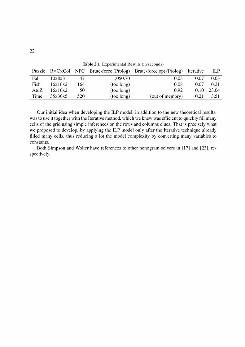
model that solves colored nonograms.The performance results of our approach compared to an adaptation for colored nonograms

of the depth-first search provided by Hett [10], an adapted version of the optimized depth-firstsearch approach also by Hett and Olšák’s grid are shown in table 2.1.

The times were measured on a 2.4 GHz Intel© Centrino© vPro™with 2 GB of RAM runningMicrosoft© Windows©. The Prolog program was run in ECLiPSe [1] and the generated ILPproblems were run on SCIP [4]. Results are shown in table 4.1, where NPC stands for "Numberof Painted Cells".

Given the good performance of the iterative approaches we also proposed to develop a hy-brid model between this approach and the ILP one.

The ILP approach presented here starts from scratch with an empty grid and, in general,could not improve the Iterative method for the available tests, although already presented similarresults using a non commercial tool.

22

Table 2.1 Experimental Results (in seconds)

Puzzle R×C×Col NPC Brute-force (Prolog) Brute-force opt (Prolog) Iterative ILPFall 10x8x3 47 1,050.70 0.03 0.07 0.03Fish 16x16x2 164 (too long) 0.08 0.07 0.21AtoZ 16x16x2 50 (too long) 0.92 0.10 23.04Time 35x30x5 520 (too long) (out of memory) 0.21 3.51

Our initial idea when developing the ILP model, in addition to the new theoretical results,was to use it together with the Iterative method, which we knew was efficient to quickly fill manycells of the grid using simple inferences on the rows and columns clues. That is precisely whatwe proposed to develop, by applying the ILP model only after the Iterative technique alreadyfilled many cells, thus reducing a lot the model complexity by converting many variables toconstants.

Both Simpson and Wolter have references to other nonogram solvers in [17] and [23], re-spectively.

3 . An ILP model for solving Colored Nonograms

In the previous chapter we verified that no ILP model for solving colored nonograms exists.In this chapter we describe the model we developed for this purpose.

3.1 Model Description

As in [7], our approach is to think of a colored nonogram as a problem comprised of twointerlocking tiling problems: one involving the placement of the row blocks, and the otherinvolving the placement of the column blocks. If a cell is painted (it can be assumed thatunpainted cells are painted white) then it must be covered by both a row block and a columnblock; if it is painted white (not painted) then it must be left uncovered by the row blocks andthe column blocks.

3.1.1 Notation

The notation used here is similar to the one used by Bosch in [7], as follows.

m = the number of rows,

n = the number of columns,

o = the number of colors excluding white (We use a sequence of natural numbers toidentify colors, starting at 1 (1,2, . . . ,o).),

bri = the number of blocks in row i, 1 ≤ i ≤ m,

bcj = the number of blocks in column j, 1 ≤ j ≤ n,

sri,1, s

ri,2, . . . , s

ri,br

i= the block-size sequence for row i,

scj,1, s

cj,2, . . . , s

cj,bc

j= the block-size sequence for column j,

cri,1,c

ri,2, . . . ,c

ri,br

i= the block-color sequence for row i,

ccj,1,c

cj,2, . . . ,c

cj,bc

j= the block-color sequence for column j.

In addition, let

eri,t = the smallest value of j such that row i’s tth block can be placed in row i with its

leftmost pixel occupying cell j,23

24

lri,t = the largest value of j such that row i’s tth block can be placed in row i with itsleftmost pixel occupying cell j,

ecj,t = the smallest value of i such that column j’s tth block can be placed in column j with

its topmost pixel occupying cell i,

lci,t = the largest value of i such that column j’s tth block can be placed in column j withits topmost pixel occupying cell i.

These are constants valid for the empty puzzle. (The letters "e" and "l" stand for "earliest"and "latest"). In our example puzzle, the second row’s first block must be placed so that itsleftmost pixel occupies cell 1 or 2, the second block must be placed so that its leftmost pixeloccupies cell 5 or 6, and the third block must be placed so that its leftmost pixel occupies cell 6or 7. In other words

er2,1 = 1, lr2,1 = 2,er

2,2 = 5, lr2,2 = 6,er2,3 = 6 and lr2,3 = 7.

These values are obtained by iteratively placing the blocks in their leftmost or topmostpossible cells and then placing them in their rightmost or bottommost possible cells. In ourexample, the first block’s first cell is 1 and, since the first block’s size is 4 and the color of bothblocks is different, the second block’s first possible cell is 5. Then, since the color of the thirdblock is also different from the second one and the size of the second block is 1, the third block’sfirst possible cell is 6. Now, the third block is pushed to its rightmost cell (7) and one finds outthat the second block’s last possible cell is 6 and the first block’s last possible cell is 2.

Note that the rules for determining these values are the same for colored or black and whitenonograms. Of course, in black and white puzzles all the blocks are of the same color, whichmeans they have to be separated by at least one empty cell.

3.1.2 Variables

As in the approach by Bosch in [7], in our approach there are three sets of variables. One setspecifies the color of each cell:

∀1≤i≤m,1≤ j≤n zi, j =

1 ≤ c ≤ o ; if row i’s jth cell is painted

with color c0 ; if row i’s jth cell is not

painted

(3.1)

The other two sets of variables are concerned with placements of the row and column blocks.

∀1≤i≤m,1≤t≤bri ,e

ri,t≤ j≤lri,t

yi,t, j =

1

; if row i’s tth block is placedin row i with its leftmost pixeloccupying cell j

0 ; if not

(3.2)

25

∀1≤ j≤n,1≤t≤bcj,e

cj,t≤i≤lcj,t

x j,t,i =

1

; if column j’s tth block isplaced in column j with itstopmost pixel occupying celli

0 ; if not

(3.3)

3.1.3 Block constraints

To ensure that row i’s tth block appears in row i exactly once, the following imposes

∀1≤i≤m,1≤t≤bri

lri,t∑j=er

i,t

yi,t, j = 1 (3.4)

For line 2 of our example we have

y2,1,1 + y2,1,2 = 1,

y2,2,5 + y2,2,6 = 1,

y2,3,6 + y2,3,7 = 1.

For the next two constraints the auxiliary function (3.5) is defined. This function, whichwas already defined as equation 2.6 in chapter 1, returns the value 1 if the two arguments arethe same, and 0 otherwise, which will be useful to compare colors of two contiguous blocks.

eq(c1,c2) =

{1 ; if c1 = c20 ; otherwise (3.5)

To ensure that row i’s (t + 1)th block is placed to the right of its tth block, the followingimposes

∀eri,t+1≤ j≤lri,t

yi,t, j ≤

lri,t+1∑j′= j+sr

i,t+eq(cri,t,c

ri,t+1)

yi,t+1, j′ (3.6)

In line 2 of our example we have

y2,1,2 ≤ y2,2,6,

y2,2,6 ≤ y2,3,7.

To ensure that column j’s tth block appears in column j exactly once, the following imposes

26

∀1≤ j≤n,1≤t≤bcj

lcj,t∑i=ec

j,t

x j,t,i = 1 (3.7)

To ensure that column j’s (t + 1)th block is placed under its tth block, the following imposes

∀ecj,t+1≤i≤lcj,t

x j,t,i ≤

lcj,t+1∑i′=i+sc

j,t+eq(ccj,t,c

cj,t+1)

x j,t+1,i′ (3.8)

3.1.4 Double Coverage Constraints

To guarantee that each painted cell is covered by both a row block and a column block, thefollowing pair of inequalities imposes:

∀1≤i≤m,1≤ j≤n zi, j ≤

bri∑

t=1

min{lri,t, j}∑j′=max{er

i,t, j−sri,t+1}

yi,t, j′ × cri,t (3.9)

∀1≤i≤m,1≤ j≤n zi, j ≤

bcj∑

t=1

min{lcj,t,i}∑i′=max{ec

j,t,i−scj,t+1}

x j,t,i′ × ccj,t (3.10)

Without these restrictions the model would allow having cells painted by row blocks, butnot painted by any column block, or vice versa. The first inequality (3.9) states that if row i’sjth cell is painted, then at least one of row i’s blocks must be placed in such a way that it coversrow i’s jth cell. (The upper and lower limits of the second summation make sure that j′ satisfiesthe two pairs of inequalities er

i,t ≤ j′ ≤ lri,t and j− sri,t + 1 ≤ j′ ≤ j. The first pair holds if, and

only if, row i’s tth cell is covered when row i’s tth block is placed in row i with its leftmost pixeloccupying cell j′. The second pair holds if and only if row i’s jth pixel is covered when rowi’s tth block is placed in row i with its leftmost pixel occupying pixel j′). The other inequality(3.10) makes sure that if row i’s jth cell is painted, then at least one of column j’s blocks coversit. For line 2 of our example we have for cell z2,4 that

z2,5 ≤ y2,1,2× cr2,1 + y2,2,5× cr

2,2,

z2,5 ≤ x5,1,1× cc5,1 + x5,1,2× cc

5,1

If z2,5 is painted, the right hand terms of these inequalities will yield exactly its color valuein a solved puzzle. Otherwise (empty cell), the terms hold value 0. Ideally, the model shouldexpress this disjunction directly, allowing only those 2 values. However, in order to allow ILP

27

solving, it is kept as a linear inequality. Nevertheless, below it is proven that this is sufficientfor a correct and complete model, in the presence of the other constraints.

Finally, constraints that prevent unpainted cells from being covered by the row blocks orcolumn blocks are included — inequalities (3.11) and (3.12).

∀1≤i≤m, 1≤ j≤n, 1≤t≤bri , j−sr

i,t+1≤ j′≤ j, eri,t≤ j′≤lri,t

zi, j ≥ yi,t, j′ × cri,t (3.11)

∀1≤i≤m, 1≤ j≤n, 1≤t≤bcj, ec

j,t≤i′≤lcj,t, i−scj,t+1≤i′≤i zi, j ≥ x j,t,i′ × cc

j,t (3.12)

In line 2 of our example we have

z2,5 ≥ y2,1,2× cr2,1, z2,5 ≥ y2,2,5× cr

2,2,

z2,5 ≥ x5,1,1× cc5,1, z2,5 ≥ x5,1,2× cc

5,1.

One might think that it is necessary to ensure that each painted cell must be covered by onerow block and one column block of the same color. However, the remaining constraints ensurethat there is only the need to guarantee that a painted cell must be covered by one row block andone column block. In order to prove it, let us explore all the possibilities regarding the coverageof some cell z:

1. No block covers cell z;

2. Only one block covers cell z and it is of the same color;

3. Only one block covers cell z and its color is smaller than the color of z;

4. Only one block covers cell z and its color is greater than the color of z;

5. More than one block covers cell z;

Of these five possibilities, only the first two are possible in real puzzles. The last three arethe ones that our model has to avoid.

In sake of simplicity, but with no loss of generality, only inequality (3.9), for lines, of thedouble coverage constraints will be used in our case analysis for these five possibilities:

Possibility 1: The only way to satisfy this possibility is with an empty cell z, with value 0,which, by inequality (3.9), will guarantee that no block covers it (forcing the respective yi,t, j′

variables to be 0), i.e.

bri∑

t=1

max{lri,t, j}∑j′=min{er

i,t, j−sri,t+1}

yi,t, j′ × cri,t = 0.

28

Possibility 2: This possibility fully satisfies inequality (3.9), corresponding to the equality ofboth terms.

Possibility 3: If a single block of smaller color than the color of cell z covers it then inequality(3.9) is not satisfied, thus disallowing such possibility, as desired.

Possibility 4: In the case that there may be one block that covers cell z, and which color isgreater than the color of z, then inequality (3.9) would be satisfied. However, this would violateinequality (3.11) thus turning the solution invalid.

Possibility 5: If more than one block covers cell z, inequality (3.9) could only be satisfied ifthe sum of the colors of the covering blocks is less than or equal to the color of cell z. But thiswould violate equation (3.4) thus turning the solution invalid.

3.1.5 Objective Function

Since this is a satisfaction problem there is no need for an objective function, but since ILPsolvers need one, the following is included (note that this function is a constant and we alreadyknow its value):

minimize/maximizem∑

i=1

n∑j=1

zi, j (3.13)

3.1.6 Pre-conditions

We also include in our approach one pre-condition in order to verify whether the puzzle istrivially impossible to solve, before even trying to search for a solution (another improvementwith respect to [7]). This is a necessary, but not sufficient condition that will save the time oftrying to solve a puzzle that is impossible, and that also helps determining whether there is anyerror in the definition of the puzzle. This condition, shown by equation (3.14), checks whetherthe sum of the sizes of all blocks of each color is the same for both the rows and columns clues.

∀c∈{1..o}

m∑i=1

bri∑

t=1

f (sri,t,c

ri,t,c) =

n∑j=1

bcj∑

t=1

f (scj,t,c

cj,t,c) (3.14)

where f (s,c1,c2) = s if c1 = c2, and 0 otherwise.

29

3.2 Instantiation to Black and White Nonograms

If o is set to 1 (o = 1), thus allowing only black and white in a puzzle, our model becomes theone provided by Bosch in [7], i.e., equation (3.1) becomes

zi, j =

{1 ; if row i’s jth cell is painted0 ; if row i’s jth cell is not painted

(3.15)

Equations (3.2) and (3.3) are kept from the approach provided by Bosch. Equation (3.4)is equal to the one in the approach by Bosch, but inequality (3.6) was extended so block t + 1can follow block t immediately, due to possible contiguous blocks of different colors. For blackand white puzzles it corresponds exactly to the formulation in [7] since all blocks have the samecolor which leads the eq function to always yield value 1. Inequalities (3.7) and (3.8) are similar,but regard columns. Finally, since the only possible color takes value 1, the double coverageconstraints set by inequalities (3.9) and (3.10) become

∀1≤i≤m,1≤ j≤n zi, j ≤

bri∑

t=1

min{lri,t, j}∑j′=max{er

i,t, j−sri,t+1}

yi,t, j′ , (3.16)

∀1≤i≤m,1≤ j≤n zi, j ≤

bcj∑

t=1

min{lcj,t,i}∑i′=max{ec

j,t,i−scj,t+1}

x j,t,i′ , (3.17)

∀1≤i≤m,1≤ j≤n,1≤t≤bri , j−sr

i,t+1≤ j′≤ j,eri,t≤ j′≤lri,t

zi, j ≥ yi,t, j′ (3.18)

and

∀1≤i≤m,1≤ j≤n,1≤t≤bcj,e

cj,t≤i′≤lcj,t,i−sc

j,t+1≤i′≤i zi, j ≥ x j,t,i′ (3.19)

as in [7] (where the min and max functions are incorrectly swapped in the summation limits).

3.3 Finding Multiple Solutions

The described ILP model allows finding a single solution to a puzzle, which actually is the bestone, although in this case all solutions are alike since the optimizing function is a constant.

Nonograms are satisfaction problems, which in ILP must be modeled as optimization prob-lems. Since it is possible that the obtained solution is not unique, we also try to find additionalsolutions to a puzzle. For that, the algorithm developed by Jung-Fa Tsai et al. described in [18]was first considered. This algorithm uses an integer cut to exclude the previously found solu-tion, extending the ILP model to a Mixed ILP model (MILP), which is the general approach tofinding additional solutions in ILP. But, in fact, a much simpler approach was used by applyinga binary cut similar to the one proposed by Balas and Jeroslow in [5].

30

Since our binary variables (either yi,t, j or x j,t,i) are enough to provide the solution (theycompletely determine the filled puzzle, since clues are constant), a binary cut is enough.

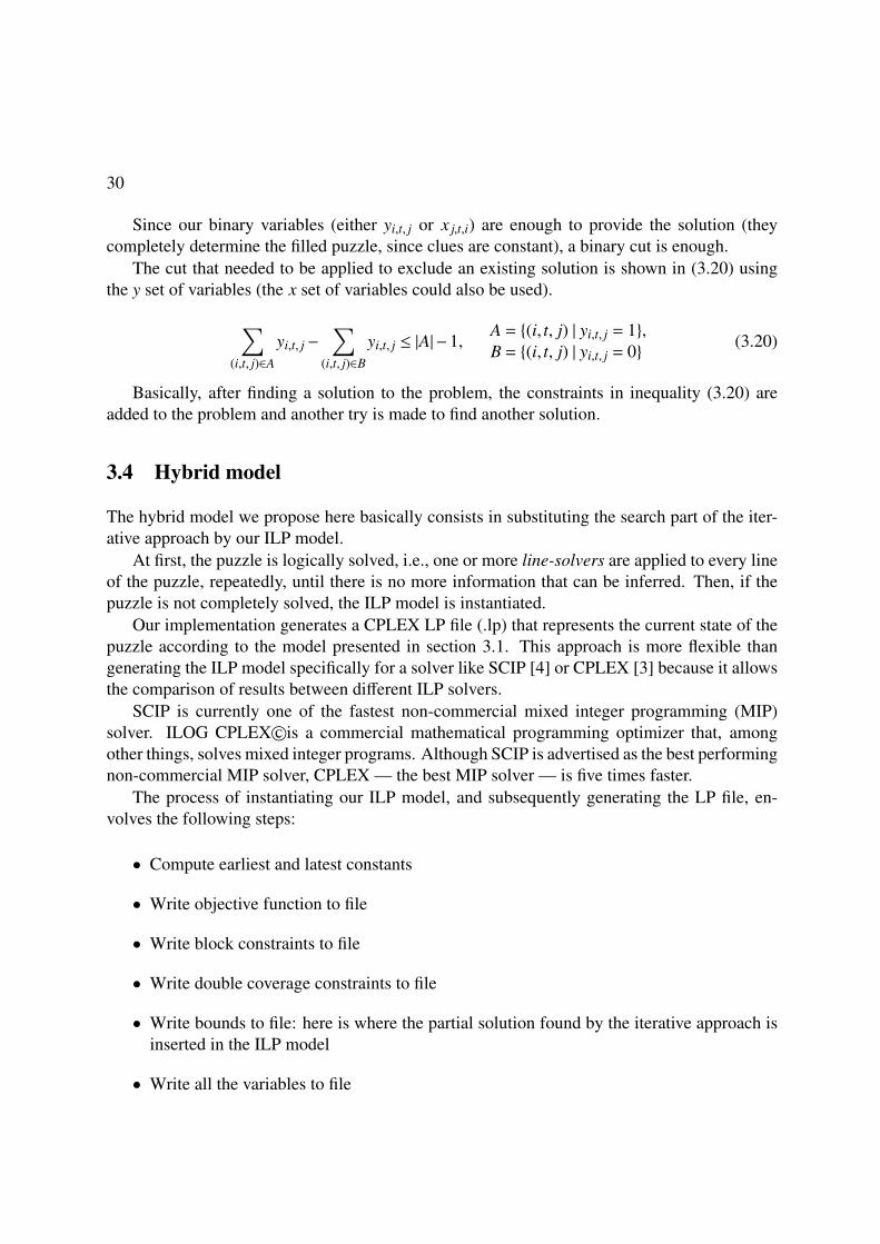
The cut that needed to be applied to exclude an existing solution is shown in (3.20) usingthe y set of variables (the x set of variables could also be used).

∑(i,t, j)∈A

yi,t, j−∑

(i,t, j)∈B

yi,t, j ≤ |A| −1,A = {(i, t, j) | yi,t, j = 1},B = {(i, t, j) | yi,t, j = 0} (3.20)

Basically, after finding a solution to the problem, the constraints in inequality (3.20) areadded to the problem and another try is made to find another solution.

3.4 Hybrid model

The hybrid model we propose here basically consists in substituting the search part of the iter-ative approach by our ILP model.

At first, the puzzle is logically solved, i.e., one or more line-solvers are applied to every lineof the puzzle, repeatedly, until there is no more information that can be inferred. Then, if thepuzzle is not completely solved, the ILP model is instantiated.

Our implementation generates a CPLEX LP file (.lp) that represents the current state of thepuzzle according to the model presented in section 3.1. This approach is more flexible thangenerating the ILP model specifically for a solver like SCIP [4] or CPLEX [3] because it allowsthe comparison of results between different ILP solvers.

SCIP is currently one of the fastest non-commercial mixed integer programming (MIP)solver. ILOG CPLEX©is a commercial mathematical programming optimizer that, amongother things, solves mixed integer programs. Although SCIP is advertised as the best performingnon-commercial MIP solver, CPLEX — the best MIP solver — is five times faster.

The process of instantiating our ILP model, and subsequently generating the LP file, en-volves the following steps:

• Compute earliest and latest constants

• Write objective function to file

• Write block constraints to file

• Write double coverage constraints to file

• Write bounds to file: here is where the partial solution found by the iterative approach isinserted in the ILP model

• Write all the variables to file

31

Since among the best performing implementations of the iterative approach only pbnsolveand Olšák’s (grid) can solve colored nonograms, we decided to adapt pbnsolve into our hybridapproach. The reason we did not choose grid was that the program code comments are inCzech. On the other hand, pbnsolve’s code comments are very complete and understandable.Steven Simpson’s nonogram [16] can not solve colored nonograms.

Also, for testing purposes, we did not implement Balas and Jeroslow’s binary cut in thisapproach.

4 . Results

In the previous chapter our ILP model for solving colored nonograms was described. Wealso described an hybrid approach to solving colored nonograms between the iterative and theILP ones.

Here, we present the results of the performance tests we ran in order to compare the differentapproaches to solving colored nonograms.

First we present the results between our pure ILP approach and the iterative and the depth-first search ones. Then we show the results obtained by comparing our hybrid approach and theiterative one.

4.1 Pure ILP approach

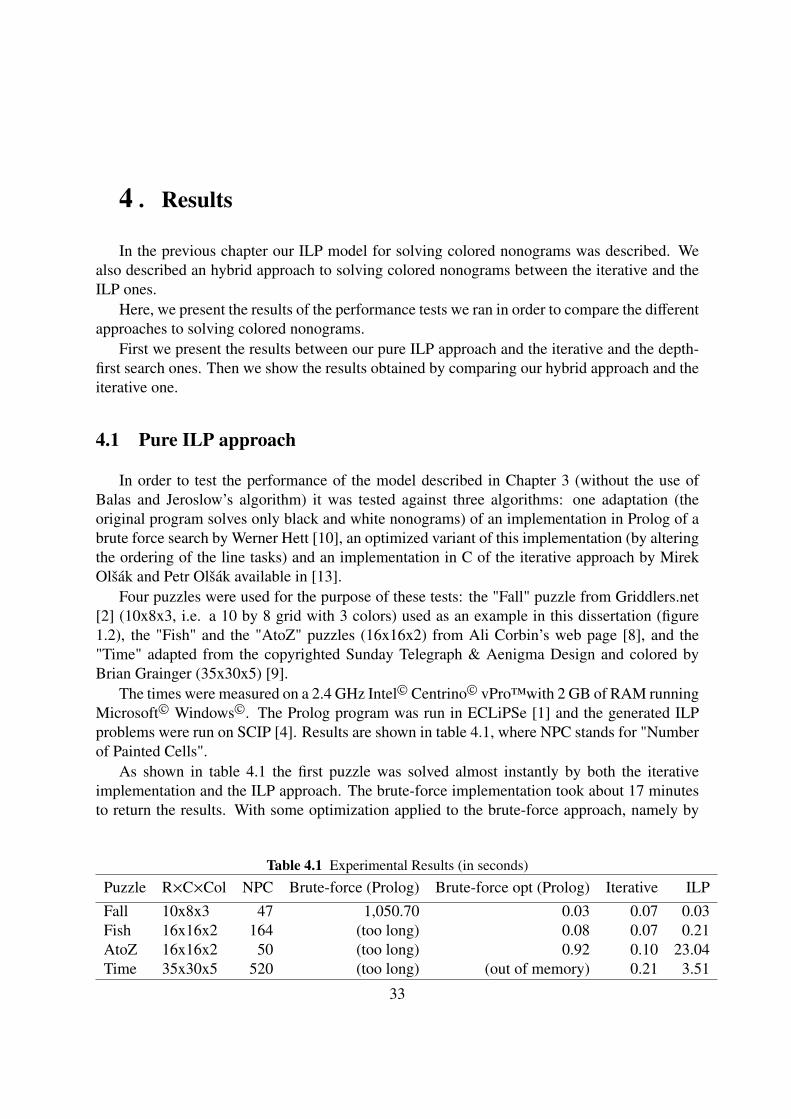
In order to test the performance of the model described in Chapter 3 (without the use ofBalas and Jeroslow’s algorithm) it was tested against three algorithms: one adaptation (theoriginal program solves only black and white nonograms) of an implementation in Prolog of abrute force search by Werner Hett [10], an optimized variant of this implementation (by alteringthe ordering of the line tasks) and an implementation in C of the iterative approach by MirekOlšák and Petr Olšák available in [13].

Four puzzles were used for the purpose of these tests: the "Fall" puzzle from Griddlers.net[2] (10x8x3, i.e. a 10 by 8 grid with 3 colors) used as an example in this dissertation (figure1.2), the "Fish" and the "AtoZ" puzzles (16x16x2) from Ali Corbin’s web page [8], and the"Time" adapted from the copyrighted Sunday Telegraph & Aenigma Design and colored byBrian Grainger (35x30x5) [9].

The times were measured on a 2.4 GHz Intel© Centrino© vPro™with 2 GB of RAM runningMicrosoft© Windows©. The Prolog program was run in ECLiPSe [1] and the generated ILPproblems were run on SCIP [4]. Results are shown in table 4.1, where NPC stands for "Numberof Painted Cells".

As shown in table 4.1 the first puzzle was solved almost instantly by both the iterativeimplementation and the ILP approach. The brute-force implementation took about 17 minutesto return the results. With some optimization applied to the brute-force approach, namely by

Table 4.1 Experimental Results (in seconds)

Puzzle R×C×Col NPC Brute-force (Prolog) Brute-force opt (Prolog) Iterative ILPFall 10x8x3 47 1,050.70 0.03 0.07 0.03Fish 16x16x2 164 (too long) 0.08 0.07 0.21AtoZ 16x16x2 50 (too long) 0.92 0.10 23.04Time 35x30x5 520 (too long) (out of memory) 0.21 3.51

33

34

Table 4.2 Results of adding equation (4.1) to ILP (in seconds)

Puzzle ILP ILP w/ ACFall 0.03 0.03Fish 0.21 0.11AtoZ 23.04 33.58Time 3.51 2.45

re-sorting the line tasks, the puzzle is also solved almost instantly. The "Fish" puzzle is a littleharder to solve. The brute-force approach was not able to solve it in a timely fashion althoughall other approaches solved it pretty quickly. The other 16x16 puzzle — "AtoZ" — is evenharder to solve. This was the hardest puzzle to solve by the ILP approach. The fourth (andbiggest) puzzle could not be solved by the brute-force algorithms. The iterative approach foundall 14 solutions to the puzzle in less than half a second and the ILP approach took about 3.5seconds to find the fist one.

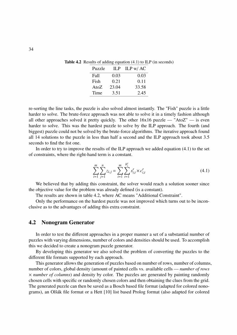
In order to try to improve the results of the ILP approach we added equation (4.1) to the setof constraints, where the right-hand term is a constant.

m∑i=1

n∑j=1

zi, j =

m∑i=1

bri∑

t=1

sri,t × cr

i,t (4.1)

We believed that by adding this constraint, the solver would reach a solution sooner sincethe objective value for the problem was already defined (is a constant).

The results are shown in table 4.2, where AC means "Additional Constraint".Only the performance on the hardest puzzle was not improved which turns out to be incon-

clusive as to the advantages of adding this extra constraint.

4.2 Nonogram Generator

In order to test the different approaches in a proper manner a set of a substantial number ofpuzzles with varying dimensions, number of colors and densities should be used. To accomplishthis we decided to create a nonogram puzzle generator.

By developing this generator we also solved the problem of converting the puzzles to thedifferent file formats supported by each approach.

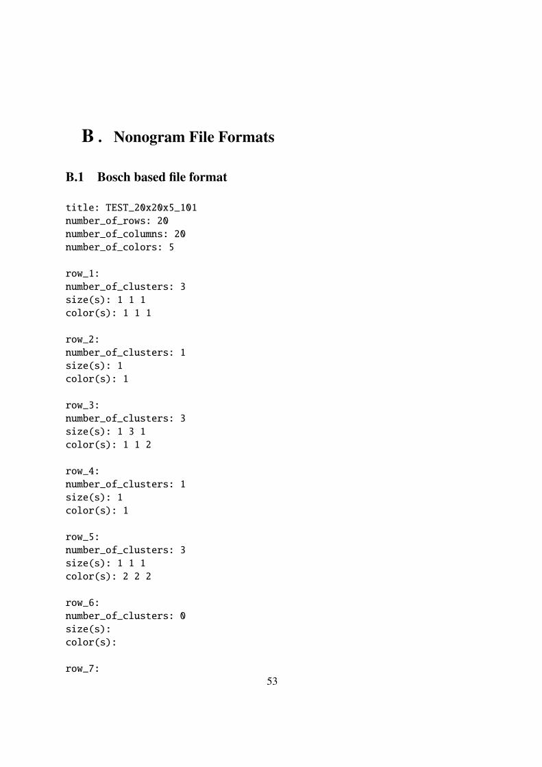
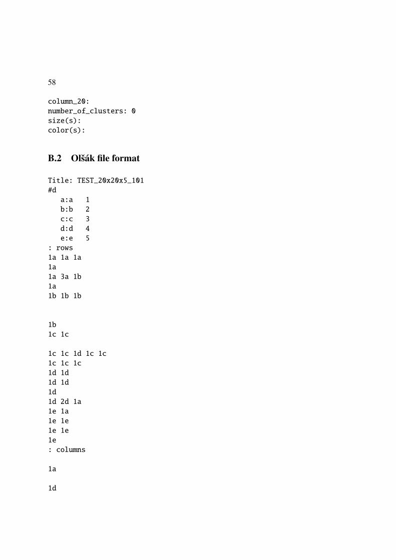
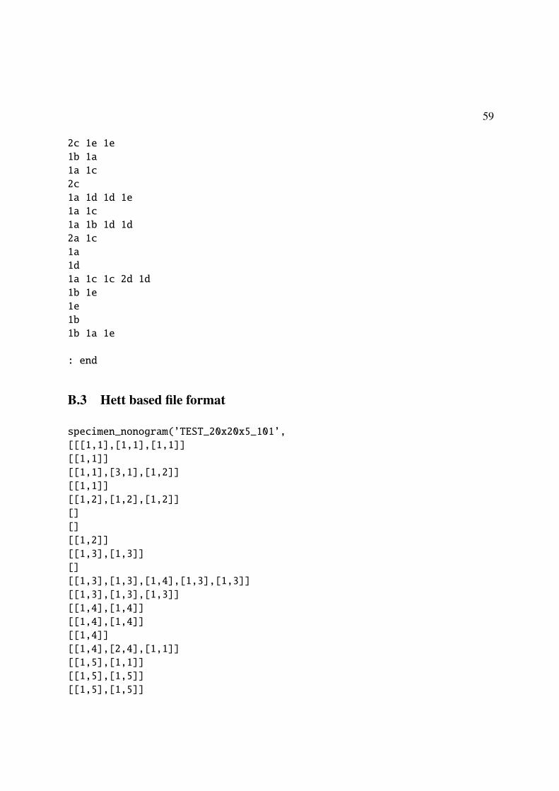
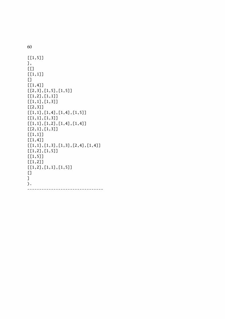
This generator allows the generation of puzzles based on number of rows, number of columns,number of colors, global density (amount of painted cells vs. available cells — number of rows× number of columns) and density by color. The puzzles are generated by painting randomlychosen cells with specific or randomly chosen colors and then obtaining the clues from the grid.The generated puzzle can then be saved as a Bosch based file format (adapted for colored nono-grams), an Olšák file format or a Hett [10] list based Prolog format (also adapted for colored

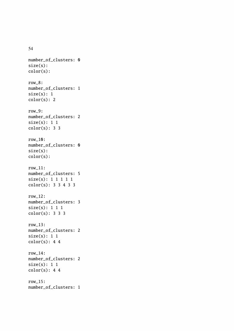
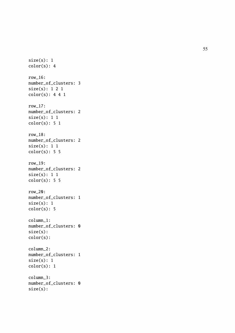
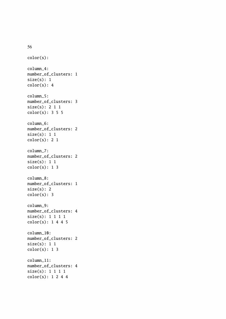
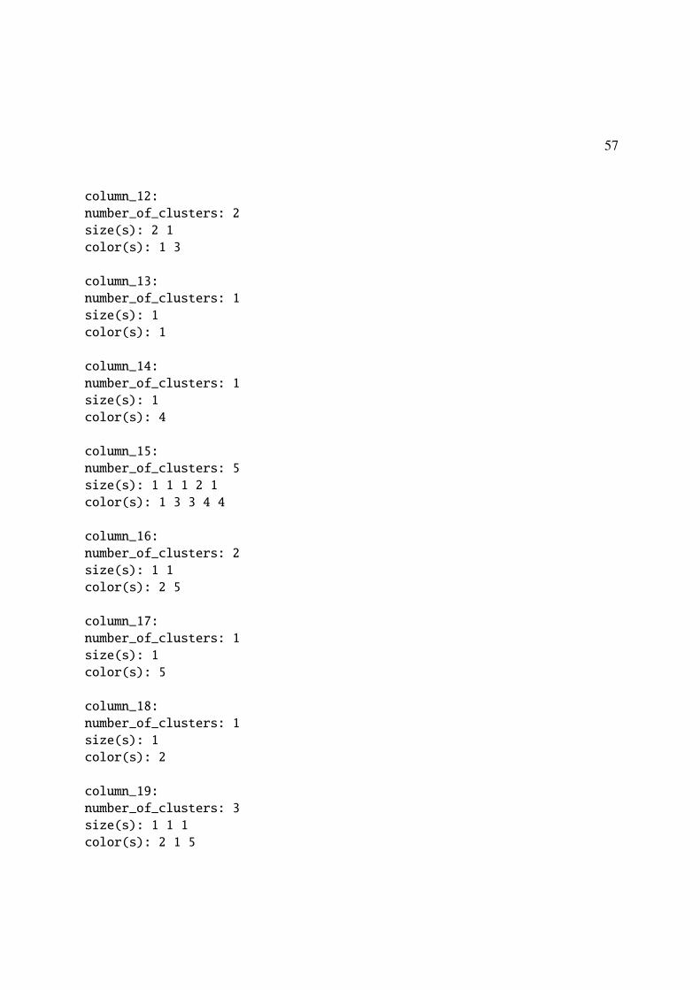
35

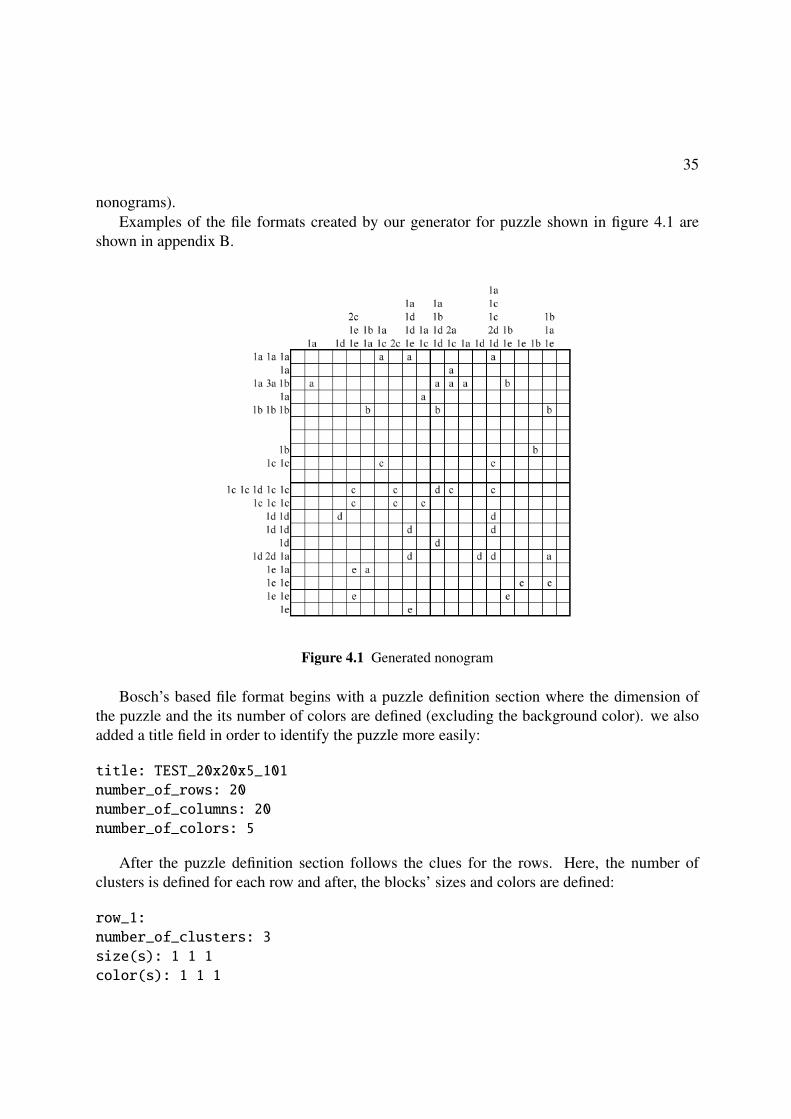
nonograms).Examples of the file formats created by our generator for puzzle shown in figure 4.1 are

shown in appendix B.

Figure 4.1 Generated nonogram

Bosch’s based file format begins with a puzzle definition section where the dimension ofthe puzzle and the its number of colors are defined (excluding the background color). we alsoadded a title field in order to identify the puzzle more easily:

title: TEST_20x20x5_101number_of_rows: 20number_of_columns: 20number_of_colors: 5

After the puzzle definition section follows the clues for the rows. Here, the number ofclusters is defined for each row and after, the blocks’ sizes and colors are defined:

row_1:number_of_clusters: 3size(s): 1 1 1color(s): 1 1 1

36

The last section of the file defines the clues for the columns and its format is similar to theprevious one.

In Olšák’s file format all text before "#" or ":" in the first column is ignored. If the puzzlehas colored blocks then we need to write "#D" or "#d" in the first column.

This line denotes the start of the color declaration. The color declaration ends by a ":" in thefirst column and the block declarations follow at the next line immediately.

Lines of color declarations have the following format:<spaces><inchar><colon><outchar><spaces><word_XPM><spaces><comment>The < spaces> denotes zero or more spaces or tabs. The exception: <word_XPM> has to

be terminated by one or more spaces and/or tabs.<inchar> is a character used to identify a color in the block declaration section, after the

numbers that represent their sizes. digits, spaces, commas or tab can not be used for <inchar>declaration. The "0" and "1" are exceptions, see bellow.<outchar> is a character which will be used to represent that color in the terminal printing

of the solution.<word_XPM> is the word (without spaces) used in XPM format for color declaration. we

can use the natural word for the color (e.g. blue) or a six hexadecimal digits preceded by a "#"that represents a RGB color (e.g. "#0000FF"). In order to use a natural word for colors theyhave to be defined in the rgb.txt of the X window system where program runs.

If <inchar> is "0", then this line declares the color for the background of the image. If thisdeclaration is omitted white will be used as the background color.

If <inchar> is "1", then this line declares the "default" color of blocks. This color is usedif no <inchar> follows the block declaration. If this line is omitted then the color must bespecified for each block declaration.

Each block declaration section (one for row and one for columns) begins after a line with acolon. For every line of the puzzle a sequence of size and color pairs (without spaces separatingthe size and the color) separated by spaces or tabs.

Hett’s based file format is defined as a predicate with three arguments: a title and two lists.Each list defines the list of blocks for rows and columns and is composed of a list of blocks thatcan be empty. Each block is another list with two elements: a size and a color.

4.3 Hybrid ILP approach

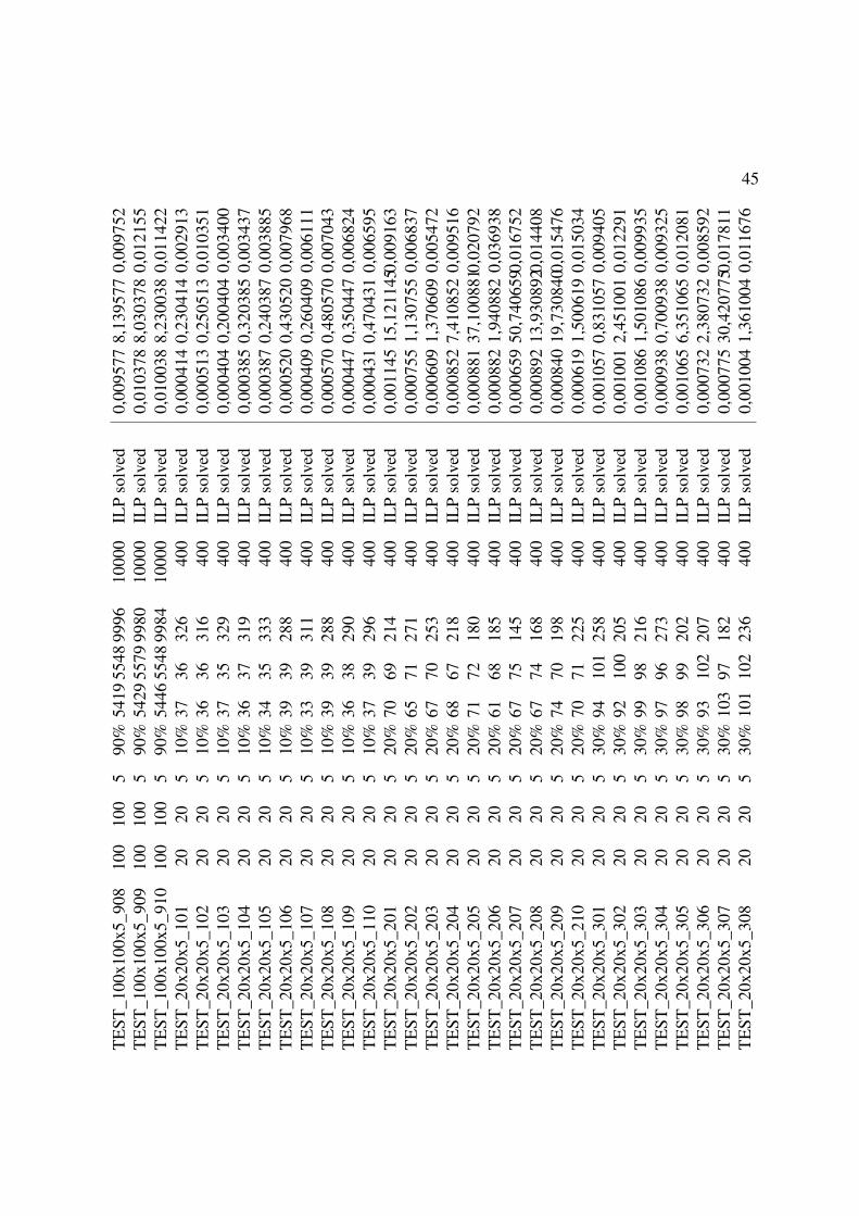
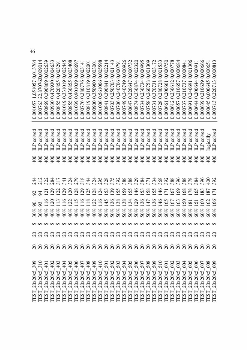
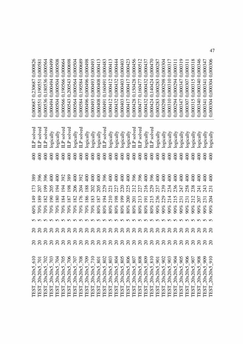
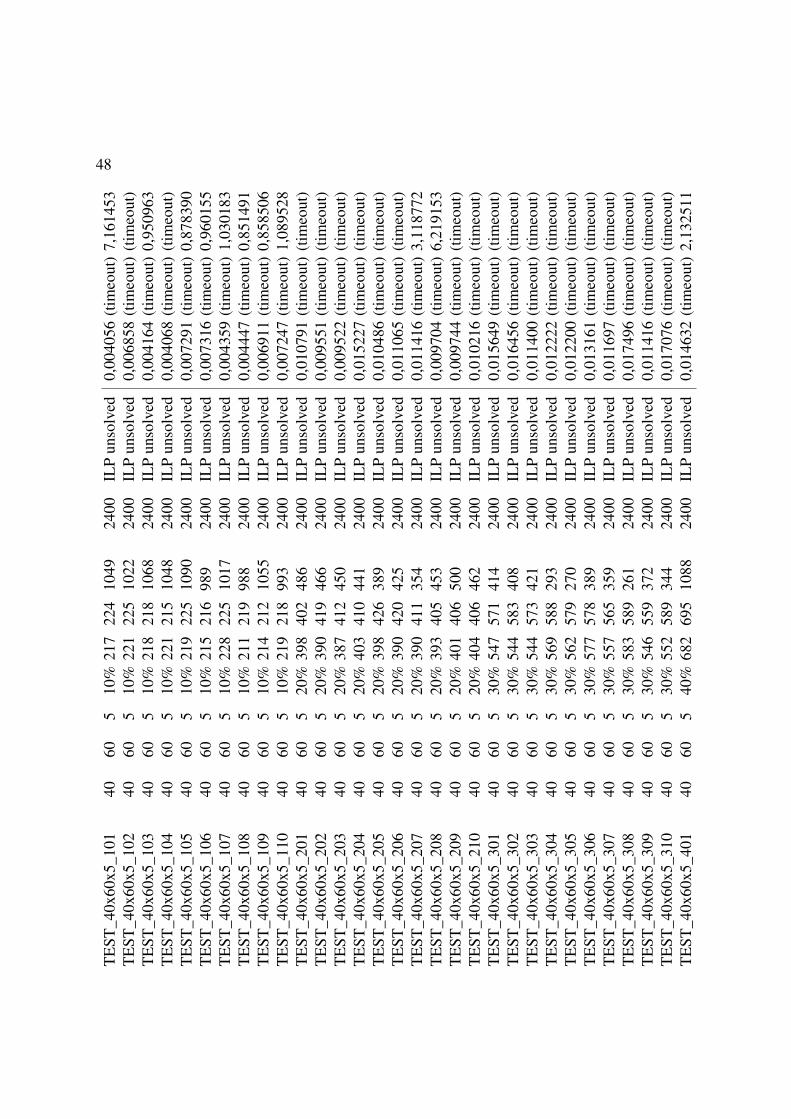
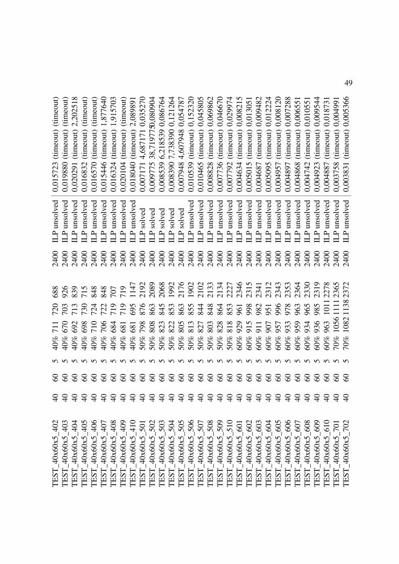
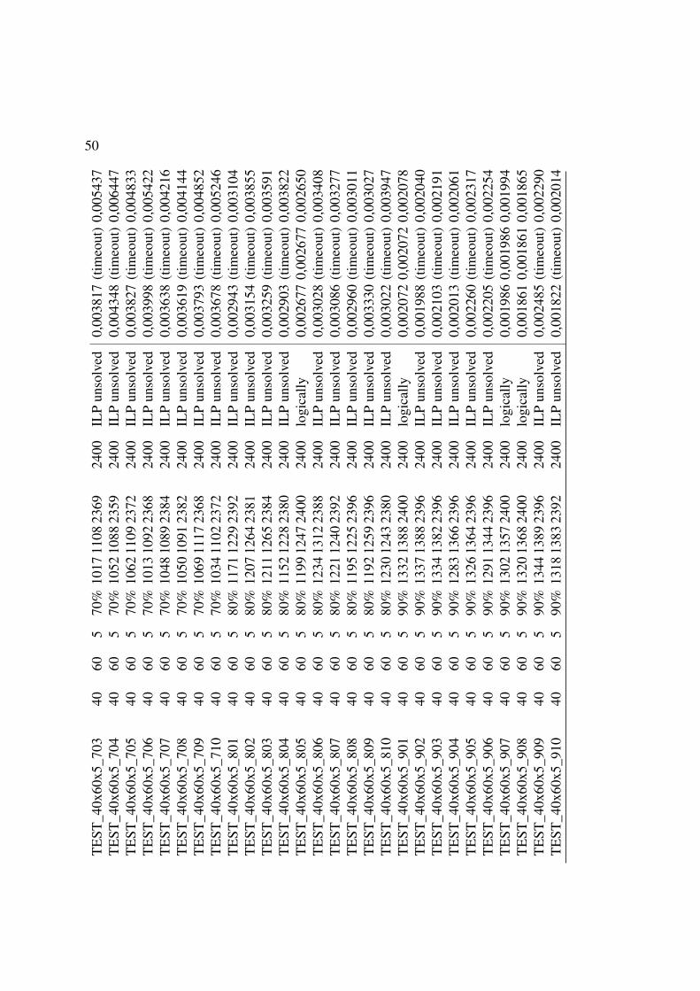
For the purpose of this work 270 problems were generated divided in three large subsetsof 20×20×5 (number of rows by number of columns with number of colors), 40×60×5 and100×100×5. Each of these subsets contains 90 problems divided by density (10 of each density— 10%, 20%, 30%, 40%, 50%, 60%, 70%, 80% and 90%).

This hybrid ILP solution was tested against pbnsolve — the implementation in C of theiterative approach by Jan Wolter available in [22]. Due to the poor results shown by the Prologimplementations by Werner Hett [10] they were removed from this test.

37

We imposed a time limit of 15 minutes for solving each of the puzzles in both approaches.The results were not the ones we expected. The iterative approach is still the fastest to

solve colored nonograms and was the one that solved more nonograms within the 15 minutestimeframe we imposed. Also, in terms of memory consumption, the iterative approach is better.Although the save and load times of the .lp files generated from our sample set of nonogramswere not taken into account, some were over 100 MB in size. This means that if these timeswere added the results would be worse. Of course, if these times were taken into account wewould be penalizing the ILP model with hard disk access (much slower than memory access).A solution to this problem would be to completely integrate the hybrid approach, i.e., withoutgenerating any files.

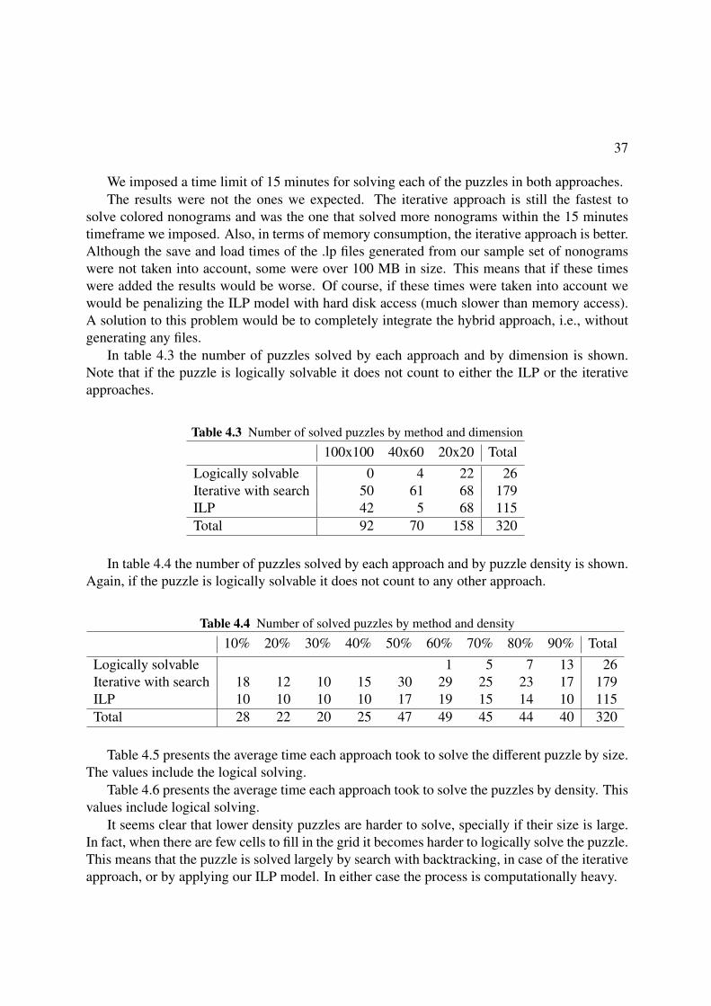
In table 4.3 the number of puzzles solved by each approach and by dimension is shown.Note that if the puzzle is logically solvable it does not count to either the ILP or the iterativeapproaches.

Table 4.3 Number of solved puzzles by method and dimension

100x100 40x60 20x20 TotalLogically solvable 0 4 22 26Iterative with search 50 61 68 179ILP 42 5 68 115Total 92 70 158 320

In table 4.4 the number of puzzles solved by each approach and by puzzle density is shown.Again, if the puzzle is logically solvable it does not count to any other approach.

Table 4.4 Number of solved puzzles by method and density

10% 20% 30% 40% 50% 60% 70% 80% 90% TotalLogically solvable 1 5 7 13 26Iterative with search 18 12 10 15 30 29 25 23 17 179ILP 10 10 10 10 17 19 15 14 10 115Total 28 22 20 25 47 49 45 44 40 320

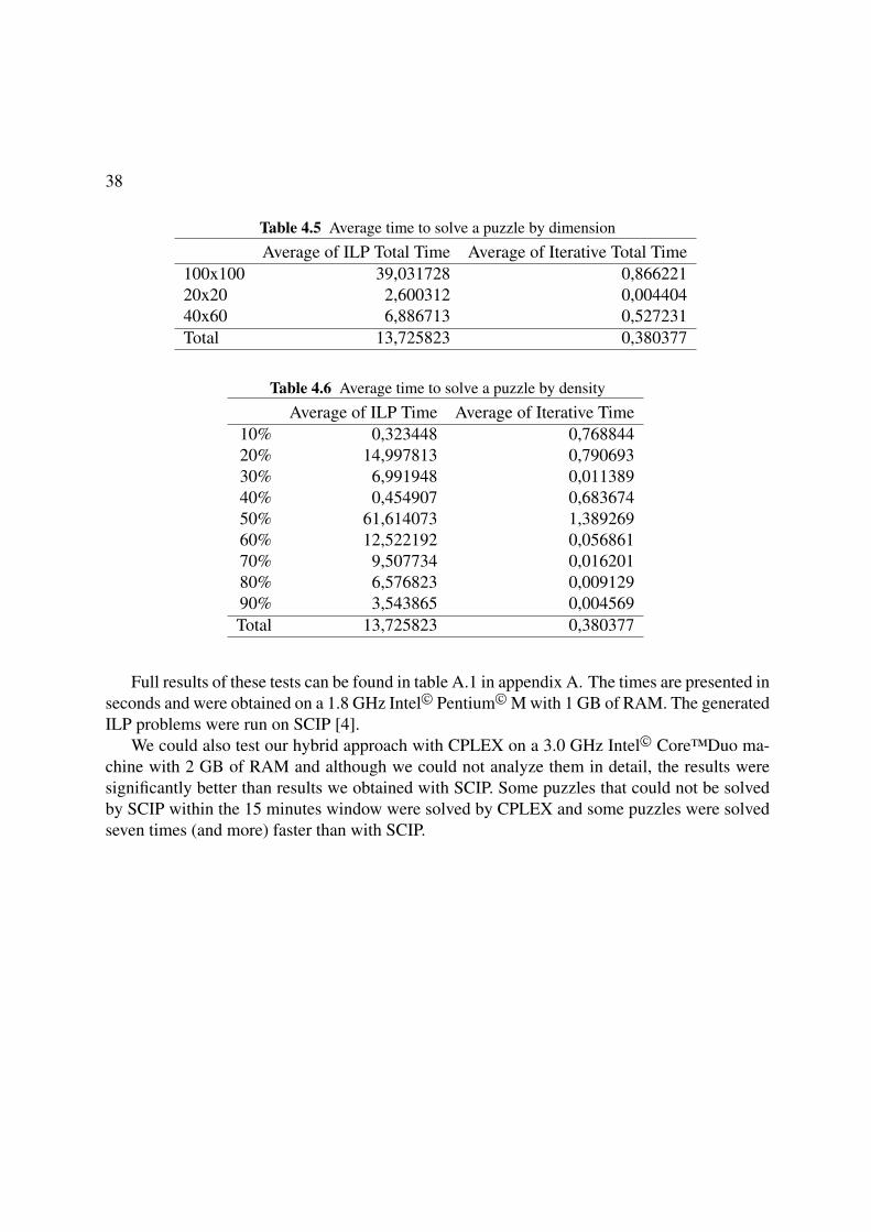
Table 4.5 presents the average time each approach took to solve the different puzzle by size.The values include the logical solving.

Table 4.6 presents the average time each approach took to solve the puzzles by density. Thisvalues include logical solving.

It seems clear that lower density puzzles are harder to solve, specially if their size is large.In fact, when there are few cells to fill in the grid it becomes harder to logically solve the puzzle.This means that the puzzle is solved largely by search with backtracking, in case of the iterativeapproach, or by applying our ILP model. In either case the process is computationally heavy.

38

Table 4.5 Average time to solve a puzzle by dimension

Average of ILP Total Time Average of Iterative Total Time100x100 39,031728 0,86622120x20 2,600312 0,00440440x60 6,886713 0,527231Total 13,725823 0,380377

Table 4.6 Average time to solve a puzzle by density

Average of ILP Time Average of Iterative Time10% 0,323448 0,76884420% 14,997813 0,79069330% 6,991948 0,01138940% 0,454907 0,68367450% 61,614073 1,38926960% 12,522192 0,05686170% 9,507734 0,01620180% 6,576823 0,00912990% 3,543865 0,004569Total 13,725823 0,380377

Full results of these tests can be found in table A.1 in appendix A. The times are presented inseconds and were obtained on a 1.8 GHz Intel© Pentium©M with 1 GB of RAM. The generatedILP problems were run on SCIP [4].

We could also test our hybrid approach with CPLEX on a 3.0 GHz Intel© Core™Duo ma-chine with 2 GB of RAM and although we could not analyze them in detail, the results weresignificantly better than results we obtained with SCIP. Some puzzles that could not be solvedby SCIP within the 15 minutes window were solved by CPLEX and some puzzles were solvedseven times (and more) faster than with SCIP.

5 . Conclusions and Future Work

In this dissertation we presented a new ILP approach to model the Colored Nonogramsproblem, which generalizes a known approach which was limited to black and white Nono-grams. We demonstrated its correctness and, additionally, we also showed how to efficientlyfind possible additional solutions by a simple adaptation of a known technique using a binarycut, by taking advantage of the specificities of this problem. This work developed during thisMaster led to the publication of the article [12].

We also enhanced the aforementioned model by merging it with an iterative approach thusproviding an hybrid approach to colored nonograms.

In order to provide a significant sample set of puzzles, for test and comparisons, we alsodeveloped a nonogram generator. This generator allows us to create puzzles given their width,height, color count and density (either global or by color) and then to save them in three formats:Bosch’s variant for colored nonograms, Olšák’s format and a Hett [10] list based Prolog formatvariant for colored nonograms.

The hybrid model results were not the ones we expected. The iterative approach is still thefastest to solve colored nonograms and was the one that solved more nonograms within the 15minutes timeframe we imposed. Also, in terms of memory consumption, the iterative approachis better. Some of the .lp files generated from our largest sample nonograms were over 100 MBin size which is a consequence of the great amount of variables and constraints that consume alot of memory.

This also means that maybe there is room for improvement. First by fully integrating themodel in one tool and then by trying to fine tune the model. One example of this can be tochange the objective function and include the objective function value as a constraint and useCPLEX to verify the results. Specially for the more complex puzzles that were not solved byeither approach, within the 15 minutes window we defined.

Another way the model can be improved is by trying to implement a backtracking mecha-nism with ILP, i.e, instead of trying to find a final solution with the ILP model, we try to find apartial solution and then reapply the iterative approach the partial solution.

The model can also be improved in order to solve other problems, like triddlers.The nonogram puzzle generator developed can also be improved by allowing to take into

account the number of blocks of a puzzle. With the current approach, the puzzles generatedhave often a large number of small size blocks.

39

A . Full Results

41

42

Tabl

eA

.1:F

ullR

esul

ts(i

nse

cond

s)

Title

WH

CD

ens.H B

lks

V Blk

sC

ells

logi

-ca

llyso

lved

Cel

lsIL

Pst

ate

Log

ictim

eIL

PTo

tal

Tim

e

Iter

ativ

eTo

tal

Tim

e

TE

ST_1

00x1

00x5

_101

100

100

510

%90

991

411

3710

000

ILP

unso

lved

0,07

1626

(tim

eout

)(t

imeo

ut)

TE

ST_1

00x1

00x5

_102

100

100

510

%90

892

010

1610

000

ILP

unso

lved

0,07

0137

(tim

eout

)(t

imeo

ut)

TE

ST_1

00x1

00x5

_103

100

100

510

%90

492

012

0910

000

ILP

unso

lved

0,06

3196

(tim

eout

)(t

imeo

ut)

TE

ST_1

00x1

00x5

_104

100

100

510

%91

590

413

3010

000

ILP

unso

lved

0,03

5417

(tim

eout

)(t

imeo

ut)

TE

ST_1

00x1

00x5

_105

100

100

510

%89

289

915

1210

000

ILP

unso

lved

0,06

4483

(tim

eout

)(t

imeo

ut)

TE

ST_1

00x1

00x5

_106

100

100

510

%92

990

611

9010

000

ILP

unso

lved

0,07

1708

(tim

eout

)(t

imeo

ut)

TE

ST_1

00x1

00x5

_107

100

100

510

%91

389

915

2710

000

ILP

unso

lved

0,03

4598

(tim

eout

)(t

imeo

ut)

TE

ST_1

00x1

00x5

_108

100

100

510

%91

889

912

2710

000

ILP

unso

lved

0,06

5956

(tim

eout

)(t

imeo

ut)

TE

ST_1

00x1

00x5

_109

100

100

510

%89

991

810

4110

000

ILP

unso

lved

0,07

0309

(tim

eout

)(t

imeo

ut)

TE

ST_1

00x1

00x5

_110

100

100

510

%92

190

510

7510

000

ILP

unso

lved

0,06

7073

(tim

eout

)(t

imeo

ut)

TE

ST_1

00x1

00x5

_201

100

100

520

%16

7016

7425

710

000

ILP

unso

lved

0,08

4544

(tim

eout

)(t

imeo

ut)

TE

ST_1

00x1

00x5

_202

100

100

520

%16

4816

8515

510

000

ILP

unso

lved

0,08

2706

(tim

eout

)(t

imeo

ut)

TE

ST_1

00x1

00x5

_203

100

100

520

%16

7016

9120

910

000

ILP

unso

lved

0,08

1917

(tim

eout

)(t

imeo

ut)

TE

ST_1

00x1

00x5

_204

100

100

520

%16

7416

4217

210

000

ILP

unso

lved

0,08

3765

(tim

eout

)(t

imeo

ut)

TE

ST_1

00x1

00x5

_205

100

100

520

%16

6616

8022

110

000

ILP

unso

lved

0,07

8765

(tim

eout

)(t

imeo

ut)

TE

ST_1

00x1

00x5

_206

100

100

520

%17

0416

8614

510

000

ILP

unso

lved

0,09

1690

(tim

eout

)(t

imeo

ut)

TE

ST_1

00x1

00x5

_207

100

100

520

%16

7316

9412

610

000

ILP

unso

lved

0,08

4892

(tim

eout

)(t

imeo

ut)

TE

ST_1

00x1

00x5

_208

100

100

520

%16

7817

0722

610

000

ILP

unso

lved

0,08

1119

(tim

eout

)(t

imeo

ut)

TE

ST_1

00x1

00x5

_209

100

100

520

%16

8416

8127

910

000

ILP

unso

lved

0,07

9904

(tim

eout

)(t

imeo

ut)

TE

ST_1

00x1

00x5

_210

100

100

520

%16

4916

8121

910

000

ILP

unso

lved

0,08

5691

(tim

eout

)(t

imeo

ut)

TE

ST_1

00x1

00x5

_301

100

100

530

%22

7823

5919

110

000

ILP

unso

lved

0,08

5262

(tim

eout

)(t

imeo

ut)

TE

ST_1

00x1

00x5

_302

100

100

530

%23

1823

5020

010

000

ILP

unso

lved

0,11

8743

(tim

eout

)(t

imeo

ut)

TE

ST_1

00x1

00x5

_303

100

100

530

%23

0623

3319

410

000

ILP

unso

lved

0,08

4814

(tim

eout

)(t

imeo

ut)

TE

ST_1

00x1

00x5

_304

100

100

530

%23

4423

2920

910

000

ILP

unso

lved

0,08

6428

(tim

eout

)(t

imeo

ut)

TE

ST_1

00x1

00x5

_305

100

100

530

%22

9823

1919

710

000

ILP

unso

lved

0,08

8181

(tim

eout

)(t

imeo

ut)

43

TE

ST_1

00x1

00x5

_306

100

100

530

%22

9123

2418

110

000

ILP

unso

lved

0,08

9121

(tim

eout

)(t

imeo

ut)

TE

ST_1

00x1

00x5

_307

100

100

530

%22

6822

8820

810

000

ILP

unso

lved

0,08

6357

(tim

eout

)(t

imeo

ut)

TE

ST_1

00x1

00x5

_308

100

100

530

%22

7923

7224

910

000

ILP

unso

lved

0,08

9197

(tim

eout

)(t

imeo

ut)

TE

ST_1

00x1

00x5

_309

100

100

530

%23

1723

4214

410

000

ILP

unso

lved

0,12

5440

(tim

eout

)(t

imeo

ut)

TE

ST_1

00x1

00x5

_310

100

100

530

%22

9223

4116

510

000

ILP

unso

lved

0,08

7015

(tim

eout

)(t

imeo

ut)

TE

ST_1

00x1

00x5

_401

100

100

540

%28

2828

7653

210

000

ILP

unso

lved

0,08

3406

(tim

eout

)(t

imeo

ut)

TE

ST_1

00x1

00x5

_402

100

100

540

%28

4129

4568

710

000

ILP

unso

lved

0,13

0944

(tim

eout

)(t

imeo

ut)

TE

ST_1

00x1

00x5

_403

100

100

540

%28

5428

7650

810

000

ILP

unso

lved

0,08

9428

(tim

eout

)(t

imeo

ut)

TE

ST_1

00x1

00x5

_404

100

100

540

%28

8228

9059

310

000

ILP

unso

lved

0,08

7703

(tim

eout

)(t

imeo

ut)

TE

ST_1

00x1

00x5

_405

100

100

540

%28

6129

3276

010

000

ILP

unso

lved

0,09

0675

(tim

eout

)(t

imeo

ut)

TE

ST_1

00x1

00x5

_406

100

100

540

%28

7829

0775

110

000

ILP

unso

lved

0,12

2355

(tim

eout

)(t

imeo

ut)

TE

ST_1

00x1

00x5

_407

100

100

540

%28

9429

0072

310

000

ILP

unso

lved

0,12

2503

(tim

eout

)(t

imeo

ut)

TE

ST_1

00x1

00x5

_408

100

100

540

%28

4929

0062

010

000

ILP

unso

lved

0,15

7251

(tim

eout

)(t

imeo

ut)

TE

ST_1

00x1

00x5

_409

100

100

540

%28

5629

4344

110

000

ILP

unso

lved

0,08

6984

(tim

eout

)(t

imeo

ut)

TE

ST_1

00x1

00x5

_410

100

100

540

%28

8629

1761

210

000

ILP

unso

lved

0,12

7249

(tim

eout

)(t

imeo

ut)

TE

ST_1

00x1

00x5

_501

100

100

550

%34

3334

3575

4310

000

ILP

unso

lved

0,09

2937

(tim

eout

)6,

1702

96T

EST

_100

x100

x5_5

0210

010

05

50%

3356

3405

7796

1000

0IL

Pun

solv

ed0,

0772

49(t

imeo

ut)

4,13

6845

TE

ST_1

00x1

00x5

_503

100

100

550

%34

0234

7581

6510

000

ILP

unso

lved

0,09

7762

(tim

eout

)2,

3877

47T

EST

_100

x100

x5_5

0410

010

05

50%

3399

3497

8393

1000

0IL

Pso

lved

0,09

7296

466,

8872

962,4

1270

9T

EST

_100

x100

x5_5

0510

010

05

50%

3403

3486

8032

1000

0IL

Pun

solv

ed0,

0838

20(t

imeo

ut)

3,67

8880

TE

ST_1

00x1

00x5

_506

100

100

550

%33

4034

5072

1910

000

ILP

unso

lved

0,09

3507

(tim

eout

)6,

7500

02T

EST

_100

x100

x5_5

0710

010

05

50%

3373

3405

8286

1000

0IL

Pso

lved

0,08

2643

515,

7626

432,6

7774

2T

EST

_100

x100

x5_5

0810

010

05

50%

3397

3445

7666

1000

0IL

Pun

solv

ed0,

1047

57(t

imeo

ut)

2,67

1261

TE

ST_1

00x1

00x5

_509

100

100

550

%34

6834

9179

1010

000

ILP

unso

lved

0,08

6351

(tim

eout

)3,

0112

43T

EST

_100

x100

x5_5

1010

010

05

50%

3383

3458

7410

1000

0IL

Pun

solv

ed0,

0755

68(t

imeo

ut)

7,04

2581

TE

ST_1

00x1

00x5

_601

100

100

560

%39

2539

5797

4710

000

ILP

solv

ed0,

0283

8325

,268

3830

,143

986

TE

ST_1

00x1

00x5

_602

100

100

560

%39

7239

8997

8410

000

ILP

solv

ed0,

0290

1424

,969

0140

,126

308

TE

ST_1

00x1

00x5

_603

100

100

560

%39

0739

7497

8010

000

ILP

solv

ed0,

0310

0424

,401

0040

,135

391

TE

ST_1

00x1

00x5

_604

100

100

560

%38

8939

2797

2310

000

ILP

solv

ed0,

0292

0525

,119

2050

,196

939

TE

ST_1

00x1

00x5

_605

100

100

560

%39

1840

0698

8110

000

ILP

solv

ed0,

0290

0323

,699

0030

,075

729

TE

ST_1

00x1

00x5

_606

100

100

560

%38

4639

3097

2310

000

ILP

solv

ed0,

0287

0024

,698

7000

,183

959

44

TE

ST_1

00x1

00x5

_607

100

100

560

%39

2940

4097

2310

000

ILP

solv

ed0,

0292

8925

,849

2890

,203

829

TE

ST_1

00x1

00x5

_608

100

100

560

%38

5339

3997

2510

000

ILP

solv

ed0,

0270

1225

,377

0120

,208

551

TE

ST_1

00x1

00x5

_609

100

100

560

%39

1939

6897

2110

000

ILP

solv

ed0,

0284

6124

,858

4610

,187

681

TE

ST_1

00x1

00x5

_610

100

100

560

%39

0639

5097

9810

000

ILP

solv

ed0,

0270

7524

,247

0750

,131

486

TE

ST_1

00x1

00x5

_701

100

100

570

%43

8744

7299

0310

000

ILP

solv

ed0,

0184

2618

,738

4260

,043

642

TE

ST_1

00x1

00x5

_702

100

100

570

%42

7144

2699

3710

000

ILP

solv

ed0,

0177

5618

,437

7560

,030

240

TE

ST_1

00x1

00x5

_703

100

100

570

%43

4044

6998

9410

000

ILP

solv

ed0,

0199

0618

,509

9060

,052

573

TE

ST_1

00x1

00x5

_704

100

100

570

%43

9844

4099

4310

000

ILP

solv

ed0,

0184

5318

,768

4530

,028

317

TE

ST_1

00x1

00x5

_705

100

100

570

%43

3344

5299

1910

000

ILP

solv

ed0,

0196

7619

,009

6760

,033

532

TE

ST_1

00x1

00x5

_706

100

100

570

%44

0444

5298

9210

000

ILP

solv

ed0,

0194

8719

,009

4870

,054

427

TE

ST_1

00x1

00x5

_707

100

100

570

%43

4444

2699

3310

000

ILP

solv

ed0,

0188

9519

,198

8950

,033

170

TE

ST_1

00x1

00x5

_708

100

100

570

%43

5844

7898

9010

000

ILP

solv

ed0,

0192

0019

,349

2000

,058

385

TE

ST_1

00x1

00x5

_709

100

100

570

%44

0045

1099

2810

000

ILP

solv

ed0,

0183

4518

,898

3450

,035

825

TE

ST_1

00x1

00x5

_710

100

100

570

%44

1244

9498

9610

000

ILP

solv

ed0,

0192

1219

,279

2120

,059

264

TE

ST_1

00x1

00x5

_801

100

100

580

%49

1550

8299

4810

000

ILP

solv

ed0,

0146

9013

,764

6900

,024

836

TE

ST_1

00x1

00x5

_802

100

100

580

%48

6950

1899

2210

000

ILP

solv

ed0,

0152

0113

,985

2010

,036

287

TE

ST_1

00x1

00x5

_803

100

100

580

%49

6550

7799

7210

000

ILP

solv

ed0,

0146

7513

,884

6750

,017

973

TE

ST_1

00x1

00x5

_804

100

100

580

%48

4349

5099

6010

000

ILP

solv

ed0,

0147

6913

,484

7690

,020

390

TE

ST_1

00x1

00x5

_805

100

100

580

%49

5750

2699

5410

000

ILP

solv

ed0,

0144

6113

,594

4610

,021

018

TE

ST_1

00x1

00x5

_806

100

100

580

%49

2550

1199

5610

000

ILP

solv

ed0,

0143

4313

,964

3430

,021

563

TE

ST_1

00x1

00x5

_807

100

100

580

%48

4649

3299

6810

000

ILP

solv

ed0,

0141

4013

,544

1400

,018

527

TE

ST_1

00x1

00x5

_808

100

100

580

%48

9050

4899

3610

000

ILP

solv

ed0,

0149

6814

,064

9680

,027

588

TE

ST_1

00x1

00x5

_809

100

100

580

%49

4550

3099

7610

000

ILP

solv

ed0,

0143

4613

,454

3460

,016

940

TE

ST_1

00x1

00x5

_810

100

100

580

%48

9049

4199

3210

000

ILP

solv

ed0,

0146

8413

,754

6840

,030

590

TE

ST_1

00x1

00x5

_901

100

100

590

%54

0655

8399

9610

000

ILP

solv

ed0,

0099

728,

0199

720,

0102

25T

EST

_100

x100

x5_9

0210

010

05

90%

5432

5640

9984

1000

0IL

Pso

lved

0,00

9949

8,17

9949

0,01

1321

TE

ST_1

00x1

00x5

_903

100

100

590

%54

7555

5999

8010

000

ILP

solv

ed0,

0104

438,

3704

430,

0124

27T

EST

_100

x100

x5_9

0410

010

05

90%

5362

5496

9988

1000

0IL

Pso

lved

0,00

9765

8,17

9765

0,01

0747

TE

ST_1

00x1

00x5

_905

100

100

590

%54

7455

9899

7610

000

ILP

solv

ed0,

0101

708,

1801

700,

0127

70T

EST

_100

x100

x5_9

0610

010

05

90%

5424

5475

9988

1000

0IL

Pso

lved

0,00

9826

7,89

9826

0,01

0810

TE

ST_1

00x1

00x5

_907

100

100

590

%54

5055

8199

8410

000

ILP

solv

ed0,

0097

278,

2697

270,

0111

62

45

TE

ST_1

00x1

00x5

_908

100

100

590

%54

1955

4899

9610

000

ILP

solv

ed0,

0095

778,

1395

770,

0097

52T

EST

_100

x100

x5_9

0910

010

05

90%

5429

5579

9980

1000

0IL

Pso

lved

0,01

0378

8,03

0378

0,01

2155

TE

ST_1

00x1

00x5

_910

100

100

590

%54

4655

4899

8410

000

ILP

solv

ed0,

0100

388,

2300

380,

0114

22T

EST

_20x

20x5

_101

2020

510

%37

3632

640

0IL

Pso

lved

0,00

0414

0,23

0414

0,00

2913

TE

ST_2

0x20

x5_1

0220

205

10%

3636

316

400

ILP

solv

ed0,

0005

130,

2505

130,

0103

51T

EST

_20x

20x5

_103

2020

510

%37

3532

940

0IL

Pso

lved

0,00

0404

0,20

0404

0,00

3400

TE

ST_2

0x20

x5_1

0420

205

10%

3637

319

400

ILP

solv

ed0,

0003

850,

3203

850,

0034

37T

EST

_20x

20x5

_105

2020

510

%34

3533

340

0IL

Pso

lved

0,00

0387

0,24

0387

0,00

3885

TE

ST_2

0x20

x5_1

0620

205

10%

3939

288

400

ILP

solv

ed0,

0005

200,

4305

200,

0079

68T

EST

_20x

20x5

_107

2020

510

%33

3931

140

0IL

Pso

lved

0,00

0409

0,26

0409

0,00

6111

TE

ST_2

0x20

x5_1

0820

205

10%

3939

288

400

ILP

solv

ed0,

0005

700,

4805

700,

0070

43T

EST

_20x

20x5

_109

2020

510

%36

3829

040

0IL

Pso

lved

0,00

0447

0,35

0447

0,00

6824

TE

ST_2

0x20

x5_1

1020

205

10%

3739

296

400

ILP

solv

ed0,

0004

310,

4704

310,

0065

95T

EST

_20x

20x5

_201

2020

520

%70

6921

440

0IL

Pso

lved

0,00

1145

15,1

2114

50,0

0916

3T

EST

_20x

20x5

_202

2020

520

%65

7127

140

0IL

Pso

lved

0,00

0755

1,13

0755

0,00

6837

TE

ST_2

0x20

x5_2

0320

205

20%

6770

253

400

ILP

solv

ed0,

0006

091,

3706

090,

0054

72T

EST

_20x

20x5

_204

2020

520

%68

6721

840

0IL

Pso

lved

0,00

0852

7,41

0852

0,00

9516

TE

ST_2

0x20

x5_2

0520

205

20%

7172

180

400

ILP

solv

ed0,

0008

8137

,100

8810

,020

792

TE

ST_2

0x20

x5_2

0620

205

20%

6168

185

400

ILP

solv

ed0,

0008

821,

9408

820,

0369

38T

EST

_20x

20x5

_207

2020

520

%67

7514

540

0IL

Pso

lved

0,00

0659

50,7

4065

90,0

1675

2T

EST

_20x

20x5

_208

2020

520

%67

7416

840

0IL

Pso

lved

0,00

0892

13,9

3089

20,0

1440

8T

EST

_20x

20x5

_209

2020

520

%74

7019

840

0IL

Pso

lved

0,00

0840

19,7

3084

00,0

1547

6T

EST

_20x

20x5

_210

2020

520

%70

7122

540

0IL

Pso

lved

0,00

0619

1,50

0619

0,01

5034

TE

ST_2

0x20

x5_3

0120

205

30%

9410

125

840

0IL

Pso

lved

0,00

1057

0,83

1057

0,00

9405

TE

ST_2

0x20

x5_3

0220

205

30%

9210

020

540

0IL

Pso

lved

0,00

1001

2,45

1001

0,01

2291

TE

ST_2

0x20

x5_3

0320

205

30%

9998

216

400

ILP

solv

ed0,

0010

861,

5010

860,

0099

35T

EST

_20x

20x5

_304

2020

530

%97

9627

340

0IL

Pso

lved

0,00

0938

0,70

0938

0,00

9325

TE

ST_2

0x20

x5_3

0520

205

30%

9899

202

400

ILP

solv

ed0,

0010

656,

3510

650,

0120

81T

EST

_20x

20x5

_306

2020

530

%93

102

207

400

ILP

solv

ed0,

0007

322,

3807

320,

0085

92T

EST

_20x

20x5

_307

2020

530

%10

397

182

400

ILP

solv

ed0,

0007

7530

,420

7750

,017

811

TE

ST_2

0x20

x5_3

0820

205

30%

101

102

236

400

ILP

solv

ed0,

0010

041,

3610

040,

0116

76

46

TE

ST_2

0x20

x5_3

0920

205

30%

9092

244

400

ILP

solv

ed0,

0010

571,

0510

570,

0137

64T

EST

_20x

20x5

_310

2020

530

%93

9421

240

0IL

Pso

lved

0,00

0763

22,8

7076

30,0

0901

4T

EST

_20x

20x5

_401

2020

540

%11

612

132

240

0IL

Pso

lved

0,00

0869

0,39

0869

0,00

2639

TE

ST_2

0x20

x5_4

0220

205

40%

120

129

284

400

ILP

solv

ed0,

0009

300,

4709

300,

0046

33T

EST

_20x

20x5

_403

2020

540

%11

312

231

740

0IL

Pso

lved

0,00

0855

0,42

0855

0,00

3291

TE

ST_2

0x20

x5_4

0420

205

40%

116

129

341

400

ILP

solv

ed0,

0010

190,

3310

190,

0024

45T

EST

_20x

20x5

_405

2020

540

%12

212

032

440

0IL

Pso

lved

0,00

0855

0,43

0855

0,00

3408

TE

ST_2

0x20

x5_4

0620

205

40%

115

128

279

400

ILP

solv

ed0,

0010

390,

9010

390,

0066

97T

EST

_20x

20x5

_407

2020

540

%11

612

931

840

0IL

Pso

lved

0,00

0776

0,38

0776

0,00

3141

TE

ST_2

0x20

x5_4

0820

205

40%

118

125

344

400

ILP

solv

ed0,

0008

190,

3108

190,

0020

01T

EST

_20x

20x5

_409

2020

540

%12

212

832

440

0IL

Pso

lved

0,00

0900

0,35

0900

0,00

3001

TE

ST_2

0x20

x5_4

1020

205

40%

116

124

295

400

ILP

solv

ed0,

0010

060,

5610

060,

0055

98T

EST

_20x

20x5

_501

2020

550

%14

515

332

840

0IL

Pso

lved

0,00

0841

0,39

0841

0,00

2214

TE

ST_2

0x20

x5_5

0220

205

50%

136

139

375

400

ILP

solv

ed0,

0007

030,

2507

030,

0011

43T

EST

_20x

20x5

_503

2020

550

%13

815

539

240

0IL

Pso

lved

0,00

0706

0,24

0706

0,00

0791

TE

ST_2

0x20

x5_5

0420

205

50%

138

159

388

400

ILP

solv

ed0,

0007

490,

2407

490,

0009

26T

EST

_20x

20x5

_505

2020

550

%13

415

538

840

0IL

Pso

lved

0,00

0647

0,22

0647

0,00

0732

TE

ST_2

0x20

x5_5

0620

205

50%

129

146

329

400

ILP

solv

ed0,

0008

740,

3308

740,

0023

20T

EST

_20x

20x5

_507

2020

550

%13

615

338

440

0IL

Pso

lved

0,00

0734

0,23

0734

0,00

0995

TE

ST_2

0x20

x5_5

0820

205

50%

147

158

371

400

ILP

solv

ed0,

0007

580,

2607

580,

0013

09T

EST

_20x

20x5

_509

2020

550

%13

615

533

440

0IL

Pso

lved

0,00

0731

0,37

0731

0,00

3172

TE

ST_2

0x20

x5_5

1020

205

50%

146

146

368

400

ILP

solv

ed0,

0007

280,

2807

280,

0015

33T

EST

_20x

20x5

_601

2020

560

%16

517

139

240

0IL

Pso

lved

0,00

0661

0,20

0661

0,00

0750

TE

ST_2

0x20

x5_6

0220

205

60%

167

167

388

400

ILP

solv

ed0,

0006

120,

2306

120,

0007

78T

EST

_20x

20x5

_603

2020

560

%16

316

939

640

0IL

Pso

lved

0,00

0657

0,21

0657

0,00

0684

TE

ST_2

0x20

x5_6

0420

205

60%

150

168

388

400

ILP

solv

ed0,

0007

370,

2107

370,

0008

41T

EST

_20x

20x5

_605

2020

560

%18

117

837

840

0IL

Pso

lved

0,00

0691

0,24

0691

0,00

1306

TE

ST_2

0x20

x5_6

0620

205

60%

151

165

384

400

ILP

solv

ed0,

0006

440,

2006

440,

0009

11T

EST

_20x

20x5

_607

2020

560

%16

018

339

640

0IL

Pso

lved

0,00

0639

0,21

0639

0,00

0666

TE

ST_2

0x20

x5_6

0820

205

60%

162

187

400

400

logi

cally

0,00

0645

0,00

0645

0,00

0651

TE

ST_2

0x20

x5_6

0920

205

60%

166

171

392

400

ILP

solv

ed0,

0007

130,

2207

130,

0008

13

47

TE

ST_2

0x20

x5_6

1020

205

60%

149

173

389

400

ILP

solv

ed0,

0006

870,

2306

870,

0008

26T

EST

_20x

20x5

_701

2020

570

%18

920

739

640

0IL

Pso

lved

0,00

0551

0,19

0551

0,00

0581

TE

ST_2

0x20

x5_7

0220

205

70%

182

199

396

400

ILP

solv

ed0,

0005

360,

1805

360,

0005

64T

EST

_20x

20x5

_703

2020

570

%19

020

540

040

0lo

gica

lly0,

0004

940,

0004

940,

0004

99T

EST

_20x

20x5

_704

2020

570

%18

019

440

040

0lo

gica

lly0,

0005

040,

0005

040,

0005

08T

EST

_20x

20x5

_705

2020

570

%18

419

439

240

0IL

Pso

lved

0,00

0566

0,19

0566

0,00

0664

TE

ST_2

0x20

x5_7

0620

205

70%

187

198

389

400

ILP

solv

ed0,

0005

430,

2005

430,

0006

98T

EST

_20x

20x5

_707

2020

570

%18

220

640

040

0lo

gica

lly0,

0005

640,

0005

640,

0005

04T

EST

_20x

20x5

_708

2020

570

%17

620

439

240

0IL

Pso

lved

0,00

0584

0,19

0584

0,00

0689

TE

ST_2

0x20

x5_7

0920

205

70%

186

188

400

400

logi

cally

0,00

0496

0,00

0496

0,00

0498

TE

ST_2

0x20

x5_7

1020

205

70%

183

202

400

400

logi

cally

0,00

0493

0,00

0493

0,00

0493

TE

ST_2

0x20

x5_8

0120

205

80%

187

205

400

400

logi

cally

0,00

0408

0,00

0408

0,00

0413

TE

ST_2

0x20

x5_8

0220

205

80%

194

229

396

400

ILP

solv

ed0,

0004

910,

1604

910,

0004

83T

EST

_20x

20x5

_803

2020

580

%21

022

140

040

0lo

gica

lly0,

0004

120,

0004

120,

0004

13T

EST

_20x

20x5

_804

2020

580

%19

822

740

040

0lo

gica

lly0,

0004

320,

0004

320,

0004

44T

EST

_20x

20x5

_805

2020

580

%19

922

040

040

0lo

gica

lly0,

0004

030,

0004

030,

0004

03T

EST

_20x

20x5

_806

2020

580

%20

022

540

040

0lo

gica

lly0,

0004

170,

0004

170,

0004

23T

EST

_20x

20x5

_807

2020

580

%20

121

239

640

0IL

Pso

lved

0,00

0428

0,15

0428

0,00

0456

TE

ST_2

0x20

x5_8

0820

205

80%

213

227

396

400

ILP

solv

ed0,

0004

770,

1604

770,

0005

12T

EST

_20x

20x5

_809

2020

580

%19

121

640

040

0lo

gica

lly0,

0004

320,

0004

320,

0004

37T

EST

_20x

20x5

_810

2020

580

%21

522

939

640

0IL

Pso

lved

0,00

0424

0,14

0424

0,00

0470

TE

ST_2

0x20

x5_9

0120

205

90%

236

237

400

400

logi

cally

0,00

0283

0,00

0283

0,00

0287

TE

ST_2

0x20

x5_9

0220

205

90%

229

239

400

400

logi

cally

0,00

0298

0,00

0298

0,00

0304

TE

ST_2

0x20

x5_9

0320

205

90%

214

234

400

400

logi

cally

0,00

0310

0,00

0310

0,00

0317

TE

ST_2

0x20

x5_9

0420

205

90%

215

236

400

400

logi

cally

0,00

0294

0,00

0294

0,00

0311

TE

ST_2

0x20

x5_9

0520

205

90%

231

247

400

400

logi

cally

0,00

0347

0,00

0347

0,00

0319

TE

ST_2

0x20

x5_9

0620

205

90%

231

258

400

400

logi

cally

0,00

0307

0,00

0307

0,00

0311

TE

ST_2

0x20

x5_9

0720

205

90%

212

238

400

400

logi

cally

0,00

0315

0,00

0315

0,00

0318

TE

ST_2

0x20

x5_9

0820

205

90%

207

241

400

400

logi

cally

0,00

0340

0,00

0340

0,00

0346

TE

ST_2

0x20

x5_9

0920

205

90%

231

243

400

400

logi

cally

0,00

0341

0,00

0341

0,00

0347

TE

ST_2

0x20

x5_9

1020

205

90%

204

231

400

400

logi

cally

0,00

0304

0,00

0304

0,00

0306

48

TE

ST_4

0x60

x5_1

0140

605

10%

217

224

1049

2400

ILP

unso

lved

0,00

4056

(tim

eout

)7,

1614

53T

EST

_40x

60x5

_102

4060

510

%22

122

510

2224

00IL

Pun

solv

ed0,

0068

58(t

imeo

ut)

(tim

eout

)T

EST

_40x

60x5

_103

4060

510

%21

821

810

6824

00IL

Pun

solv

ed0,

0041

64(t

imeo

ut)

0,95

0963

TE

ST_4

0x60

x5_1

0440

605

10%

221

215

1048

2400

ILP

unso

lved

0,00

4068

(tim

eout

)(t

imeo

ut)

TE

ST_4

0x60

x5_1

0540

605

10%

219

225

1090

2400

ILP

unso

lved

0,00

7291

(tim

eout

)0,

8783

90T

EST

_40x

60x5

_106

4060

510

%21

521

698

924

00IL

Pun

solv

ed0,

0073

16(t

imeo

ut)

0,96

0155

TE

ST_4

0x60

x5_1

0740

605

10%

228

225

1017

2400

ILP

unso

lved

0,00

4359

(tim

eout

)1,

0301

83T

EST

_40x

60x5

_108

4060

510

%21

121

998

824

00IL

Pun

solv

ed0,

0044

47(t

imeo

ut)

0,85

1491

TE

ST_4

0x60

x5_1

0940

605

10%

214

212

1055

2400

ILP

unso

lved

0,00

6911

(tim

eout

)0,

8585

06T

EST

_40x

60x5

_110

4060

510

%21

921

899

324

00IL

Pun

solv

ed0,

0072

47(t

imeo

ut)

1,08

9528

TE

ST_4

0x60

x5_2

0140

605

20%

398

402

486

2400

ILP

unso

lved

0,01

0791

(tim

eout

)(t

imeo

ut)

TE

ST_4

0x60

x5_2

0240

605

20%

390

419

466

2400

ILP

unso

lved

0,00

9551

(tim

eout

)(t

imeo

ut)

TE

ST_4

0x60

x5_2

0340

605

20%

387

412

450

2400

ILP

unso

lved

0,00

9522

(tim

eout

)(t

imeo

ut)

TE

ST_4

0x60

x5_2

0440

605

20%

403

410

441

2400

ILP

unso

lved

0,01

5227

(tim

eout

)(t

imeo

ut)

TE

ST_4

0x60

x5_2

0540

605

20%

398

426

389

2400

ILP

unso

lved

0,01

0486

(tim

eout

)(t

imeo

ut)

TE

ST_4

0x60

x5_2

0640

605

20%

390

420

425

2400

ILP

unso

lved

0,01

1065

(tim

eout

)(t

imeo

ut)

TE

ST_4

0x60

x5_2

0740

605

20%

390

411

354

2400

ILP

unso

lved

0,01

1416

(tim

eout

)3,

1187

72T

EST

_40x

60x5

_208

4060

520

%39

340

545

324

00IL

Pun

solv

ed0,

0097

04(t

imeo

ut)

6,21

9153

TE

ST_4

0x60

x5_2

0940

605

20%

401

406

500

2400

ILP

unso

lved

0,00

9744

(tim

eout

)(t

imeo

ut)

TE

ST_4

0x60

x5_2

1040

605

20%

404

406

462

2400

ILP

unso

lved

0,01

0216

(tim

eout

)(t

imeo

ut)

TE

ST_4

0x60

x5_3

0140

605

30%

547

571

414

2400

ILP

unso

lved

0,01

5649

(tim

eout

)(t

imeo

ut)

TE

ST_4

0x60

x5_3

0240

605

30%

544

583

408

2400

ILP

unso

lved

0,01

6456

(tim

eout

)(t

imeo

ut)

TE

ST_4

0x60

x5_3

0340

605

30%

544

573

421

2400

ILP

unso

lved

0,01

1400

(tim

eout

)(t

imeo

ut)

TE

ST_4

0x60

x5_3

0440

605

30%

569

588

293

2400

ILP

unso

lved

0,01

2222

(tim

eout

)(t

imeo

ut)

TE

ST_4

0x60

x5_3

0540

605

30%

562

579

270

2400

ILP

unso

lved

0,01

2200

(tim

eout

)(t

imeo

ut)

TE

ST_4

0x60

x5_3

0640

605

30%

577

578

389

2400

ILP

unso

lved

0,01

3161

(tim

eout

)(t

imeo

ut)

TE

ST_4

0x60

x5_3

0740

605

30%

557

565

359

2400

ILP

unso

lved

0,01

1697

(tim

eout

)(t

imeo

ut)

TE

ST_4

0x60

x5_3

0840

605

30%

583

589

261

2400

ILP

unso

lved

0,01

7496

(tim

eout

)(t

imeo

ut)

TE

ST_4

0x60

x5_3

0940

605

30%

546

559

372

2400

ILP

unso

lved

0,01

1416

(tim

eout

)(t

imeo

ut)

TE

ST_4

0x60

x5_3

1040

605

30%

552

589

344

2400

ILP

unso

lved

0,01

7076

(tim

eout

)(t

imeo

ut)

TE

ST_4

0x60

x5_4

0140

605

40%

682

695

1088

2400

ILP

unso

lved

0,01

4632

(tim

eout

)2,

1325

11

49

TE

ST_4

0x60

x5_4

0240

605

40%

711

720

688

2400

ILP

unso

lved

0,01

5723

(tim

eout

)(t

imeo

ut)

TE

ST_4

0x60

x5_4

0340

605

40%

670

703

926

2400

ILP

unso

lved

0,01

9880

(tim

eout

)(t

imeo

ut)

TE

ST_4

0x60

x5_4

0440

605

40%

692

713

839

2400

ILP

unso

lved

0,02

0291

(tim

eout

)2,

2025

18T

EST

_40x

60x5

_405

4060

540

%69

873

071

524

00IL

Pun

solv

ed0,

0168

32(t

imeo

ut)

(tim

eout

)T

EST

_40x

60x5

_406

4060

540

%71

072

484

824

00IL

Pun

solv

ed0,

0165

70(t

imeo

ut)

(tim

eout

)T

EST

_40x

60x5

_407

4060

540

%70

672

284

824

00IL

Pun

solv

ed0,

0154

46(t

imeo

ut)

1,87

7640

TE

ST_4

0x60

x5_4

0840

605

40%

684

719

707

2400

ILP

unso

lved

0,01

6324

(tim

eout

)1,

9157

03T

EST

_40x

60x5

_409

4060

540

%68

171

971

924

00IL

Pun

solv

ed0,

0201

04(t

imeo

ut)

(tim

eout

)T

EST

_40x

60x5

_410

4060

540

%68

169

511

4724

00IL

Pun

solv

ed0,

0180

40(t

imeo

ut)

2,08

9891

TE

ST_4

0x60

x5_5

0140

605

50%

798

876

2192

2400

ILP

solv

ed0,

0071

714,

6871

710,

0352

70T

EST

_40x

60x5

_502

4060

550

%80

886

320

8924

00IL

Pso

lved

0,00

9775

38,7

1977

50,0

8090

4T

EST

_40x

60x5

_503

4060

550

%82

384

520

6824

00IL

Pso

lved

0,00

8539

6,21

8539

0,08

6764

TE

ST_4

0x60

x5_5

0440

605

50%

822

853

1992

2400

ILP

solv

ed0,

0083

907,

7383

900,

1212

64T

EST

_40x

60x5

_505

4060

550

%80

586

321

7624

00IL

Pso

lved

0,00

7948

4,60

7948

0,05

4787

TE

ST_4

0x60

x5_5

0640

605

50%

813

855

1902

2400

ILP

unso

lved

0,01

0539

(tim

eout

)0,

1523

20T

EST

_40x

60x5

_507

4060

550

%82

784

421

0224

00IL

Pun

solv

ed0,

0104

65(t

imeo

ut)

0,04

5805

TE

ST_4

0x60

x5_5

0840

605

50%

803

848

2133

2400

ILP

unso

lved

0,00

8828

(tim

eout

)0,

0698

62T

EST

_40x

60x5

_509

4060

550

%82

886

421

3424

00IL

Pun

solv

ed0,

0077

36(t

imeo

ut)

0,04

6670

TE

ST_4

0x60

x5_5

1040

605

50%

818

853

2227

2400

ILP

unso

lved

0,00

7792

(tim

eout

)0,

0299

74T

EST

_40x

60x5

_601

4060

560

%92

996

123

4624

00IL

Pun

solv

ed0,

0046

34(t

imeo

ut)

0,00

8215

TE

ST_4

0x60

x5_6

0240

605

60%

915

998

2315

2400

ILP

unso

lved

0,00

5015

(tim

eout

)0,

0130

51T

EST

_40x

60x5

_603

4060

560

%91

198

223

4124

00IL

Pun

solv

ed0,

0046

87(t

imeo

ut)

0,00

9482

TE

ST_4

0x60

x5_6

0440

605

60%

907

951

2312

2400

ILP

unso

lved

0,00

5095

(tim

eout

)0,

0122

24T

EST

_40x

60x5

_605

4060

560

%95

799

623

4324

00IL

Pun

solv

ed0,

0049

57(t

imeo

ut)

0,00

8120

TE

ST_4

0x60

x5_6

0640

605

60%

933

978

2353

2400

ILP

unso

lved

0,00

4897

(tim

eout

)0,

0072

88T

EST

_40x

60x5

_607

4060

560

%95

996

323

6424

00IL

Pun

solv

ed0,

0048

68(t

imeo

ut)

0,00

6551

TE

ST_4

0x60

x5_6

0840

605

60%

934

965

2330

2400

ILP

unso

lved

0,00

4742

(tim

eout

)0,

0105

51T

EST

_40x

60x5

_609

4060

560

%93

698

523

1924

00IL

Pun

solv

ed0,

0049

23(t

imeo

ut)

0,00

9544

TE

ST_4

0x60

x5_6

1040

605

60%

963

1011

2278

2400

ILP

unso

lved

0,00

4887

(tim

eout

)0,

0187

31T

EST

_40x

60x5

_701

4060

570

%10

5611

1123

6524

00IL

Pun

solv

ed0,

0037

58(t

imeo

ut)

0,00

4991

TE

ST_4

0x60

x5_7

0240

605

70%

1082

1138

2372

2400

ILP

unso

lved

0,00

3831

(tim

eout

)0,

0053

66

50

TE

ST_4

0x60

x5_7

0340

605

70%

1017

1108

2369

2400

ILP

unso

lved

0,00

3817

(tim

eout

)0,

0054

37T

EST

_40x

60x5

_704

4060

570

%10

5210

8823

5924

00IL

Pun

solv

ed0,

0043

48(t

imeo

ut)

0,00

6447

TE

ST_4

0x60

x5_7

0540

605

70%

1062

1109

2372

2400

ILP

unso

lved

0,00

3827

(tim

eout

)0,

0048

33T

EST

_40x

60x5

_706

4060

570

%10

1310

9223

6824

00IL

Pun

solv

ed0,

0039

98(t

imeo

ut)

0,00

5422

TE

ST_4

0x60

x5_7

0740

605

70%

1048

1089

2384

2400

ILP

unso

lved

0,00

3638

(tim

eout

)0,

0042

16T

EST

_40x

60x5

_708

4060

570

%10

5010

9123

8224

00IL

Pun

solv

ed0,

0036

19(t

imeo

ut)

0,00

4144

TE

ST_4

0x60

x5_7

0940

605

70%

1069

1117

2368

2400

ILP

unso

lved

0,00

3793

(tim

eout

)0,

0048

52T

EST

_40x

60x5

_710

4060

570

%10

3411

0223

7224

00IL

Pun

solv

ed0,

0036

78(t

imeo

ut)

0,00

5246

TE

ST_4

0x60

x5_8

0140

605

80%

1171

1229

2392

2400

ILP

unso

lved

0,00

2943

(tim

eout

)0,

0031

04T

EST

_40x

60x5

_802

4060

580

%12

0712

6423

8124

00IL

Pun

solv

ed0,

0031

54(t

imeo

ut)

0,00

3855

TE

ST_4

0x60

x5_8

0340

605

80%

1211

1265

2384

2400

ILP

unso

lved

0,00

3259

(tim

eout

)0,

0035

91T

EST

_40x

60x5

_804

4060

580

%11

5212

2823

8024

00IL

Pun

solv

ed0,

0029

03(t

imeo

ut)

0,00

3822

TE

ST_4

0x60

x5_8

0540

605

80%

1199

1247

2400

2400

logi

cally

0,00

2677

0,00

2677

0,00

2650

TE

ST_4

0x60

x5_8

0640

605

80%

1234

1312

2388

2400

ILP

unso

lved

0,00

3028

(tim

eout

)0,

0034

08T

EST

_40x

60x5

_807

4060

580

%12

2112

4023

9224

00IL

Pun

solv

ed0,

0030

86(t

imeo

ut)

0,00

3277

TE

ST_4

0x60

x5_8

0840

605

80%

1195

1225

2396

2400

ILP

unso

lved

0,00

2960

(tim

eout

)0,

0030

11T

EST

_40x

60x5

_809

4060

580

%11

9212

5923

9624

00IL

Pun

solv

ed0,

0033

30(t

imeo

ut)

0,00

3027

TE

ST_4

0x60

x5_8

1040

605

80%

1230

1243

2380

2400

ILP

unso

lved

0,00

3022

(tim

eout

)0,

0039

47T

EST

_40x

60x5

_901

4060

590

%13

3213

8824

0024

00lo

gica

lly0,

0020

720,

0020

720,

0020

78T

EST

_40x

60x5

_902

4060

590

%13

3713

8823

9624

00IL

Pun

solv

ed0,

0019

88(t

imeo

ut)

0,00

2040

TE

ST_4

0x60

x5_9

0340

605

90%

1334

1382

2396

2400

ILP

unso

lved

0,00

2103

(tim

eout

)0,

0021

91T

EST

_40x

60x5

_904

4060

590

%12

8313

6623

9624

00IL

Pun

solv

ed0,

0020

13(t

imeo

ut)

0,00

2061

TE

ST_4

0x60

x5_9

0540

605

90%

1326

1364

2396

2400

ILP

unso

lved

0,00

2260

(tim

eout

)0,

0023

17T

EST

_40x

60x5

_906

4060

590

%12

9113

4423

9624

00IL

Pun

solv

ed0,

0022

05(t

imeo

ut)

0,00

2254

TE

ST_4

0x60

x5_9

0740

605

90%

1302

1357

2400

2400

logi

cally

0,00

1986

0,00

1986

0,00

1994

TE

ST_4

0x60

x5_9

0840

605

90%

1320

1368

2400

2400

logi

cally

0,00

1861

0,00

1861

0,00

1865

TE

ST_4

0x60

x5_9

0940

605

90%

1344

1389

2396

2400

ILP

unso

lved

0,00

2485

(tim

eout

)0,

0022

90T

EST

_40x

60x5

_910

4060

590

%13

1813

8323

9224

00IL

Pun

solv

ed0,

0018

22(t

imeo

ut)

0,00

2014

51

Lege

nd:

Title

:Titl

eof

the

nono

gram

W:W

ithof

the

nono

gram

H:H

eigh

toft

heno

nogr

amC

:Num

bero

fcol

ors

ofth

eno

nogr

amD

ens.:

Glo

bald

ensi

tyof

the

nono

gram

HB

lks:

Num

bero

fhor

izon

talb

lock

sof

the

nono

gram

VB

lks:

Num

bero

fver

tical

bloc

ksof

the

nono

gram

Cel

lslo

gica

llyso

lved

:Num

bero

fcel

lsde

term

ined

afte

rly

solv

ing

(ful

lyor

part

ially

)the

nono

gram

Cel

ls:N

umbe

rofc

ells

ofth

eno

nogr

am(t

ypic

ally

W×

H)

ILP

stat

e:L

ogic

ally

solv

ed,I

LP

solv

edor

ILP

unso

lved

Log

ictim

e:Ti

me

spen

tlog

ical

lyso

lvin

gth

eno

nogr

amIL

PTo

talT

ime:

Tota

ltim

esp

ents

olvi

ngth

eno

nogr

amus

ing

the

hybr

id,i

nclu

ding

the

time

spen

tlog

ical

lyso

lvin

git

Iter

ativ

eTo

tal

Tim

e:To

tal

time

spen

tso

lvin

gth

eno

nogr

amus

ing

the

itera

tive

appr

oach

,in

clud

ing

the

time

spen

tlo

gica

llyso

lvin

git

B . Nonogram File Formats

B.1 Bosch based file format

title: TEST_20x20x5_101number_of_rows: 20number_of_columns: 20number_of_colors: 5

row_1:number_of_clusters: 3size(s): 1 1 1color(s): 1 1 1

row_2:number_of_clusters: 1size(s): 1color(s): 1

row_3:number_of_clusters: 3size(s): 1 3 1color(s): 1 1 2

row_4:number_of_clusters: 1size(s): 1color(s): 1

row_5:number_of_clusters: 3size(s): 1 1 1color(s): 2 2 2

row_6:number_of_clusters: 0size(s):color(s):

row_7:53

54

number_of_clusters: 0size(s):color(s):

row_8:number_of_clusters: 1size(s): 1color(s): 2

row_9:number_of_clusters: 2size(s): 1 1color(s): 3 3

row_10:number_of_clusters: 0size(s):color(s):

row_11:number_of_clusters: 5size(s): 1 1 1 1 1color(s): 3 3 4 3 3

row_12:number_of_clusters: 3size(s): 1 1 1color(s): 3 3 3

row_13:number_of_clusters: 2size(s): 1 1color(s): 4 4

row_14:number_of_clusters: 2size(s): 1 1color(s): 4 4

row_15:number_of_clusters: 1

55

size(s): 1color(s): 4

row_16:number_of_clusters: 3size(s): 1 2 1color(s): 4 4 1

row_17:number_of_clusters: 2size(s): 1 1color(s): 5 1

row_18:number_of_clusters: 2size(s): 1 1color(s): 5 5

row_19:number_of_clusters: 2size(s): 1 1color(s): 5 5

row_20:number_of_clusters: 1size(s): 1color(s): 5

column_1:number_of_clusters: 0size(s):color(s):

column_2:number_of_clusters: 1size(s): 1color(s): 1

column_3:number_of_clusters: 0size(s):

56

color(s):

column_4:number_of_clusters: 1size(s): 1color(s): 4

column_5:number_of_clusters: 3size(s): 2 1 1color(s): 3 5 5

column_6:number_of_clusters: 2size(s): 1 1color(s): 2 1

column_7:number_of_clusters: 2size(s): 1 1color(s): 1 3

column_8:number_of_clusters: 1size(s): 2color(s): 3

column_9:number_of_clusters: 4size(s): 1 1 1 1color(s): 1 4 4 5

column_10:number_of_clusters: 2size(s): 1 1color(s): 1 3

column_11:number_of_clusters: 4size(s): 1 1 1 1color(s): 1 2 4 4

57

column_12:number_of_clusters: 2size(s): 2 1color(s): 1 3

column_13:number_of_clusters: 1size(s): 1color(s): 1

column_14:number_of_clusters: 1size(s): 1color(s): 4

column_15:number_of_clusters: 5size(s): 1 1 1 2 1color(s): 1 3 3 4 4

column_16:number_of_clusters: 2size(s): 1 1color(s): 2 5

column_17:number_of_clusters: 1size(s): 1color(s): 5

column_18:number_of_clusters: 1size(s): 1color(s): 2

column_19:number_of_clusters: 3size(s): 1 1 1color(s): 2 1 5

58

column_20:number_of_clusters: 0size(s):color(s):

B.2 Olšák file format

Title: TEST_20x20x5_101#da:a 1b:b 2c:c 3d:d 4e:e 5

: rows1a 1a 1a1a1a 3a 1b1a1b 1b 1b

1b1c 1c

1c 1c 1d 1c 1c1c 1c 1c1d 1d1d 1d1d1d 2d 1a1e 1a1e 1e1e 1e1e: columns

1a

1d

59

2c 1e 1e1b 1a1a 1c2c1a 1d 1d 1e1a 1c1a 1b 1d 1d2a 1c1a1d1a 1c 1c 2d 1d1b 1e1e1b1b 1a 1e

: end

B.3 Hett based file format

specimen_nonogram(’TEST_20x20x5_101’,[[[1,1],[1,1],[1,1]][[1,1]][[1,1],[3,1],[1,2]][[1,1]][[1,2],[1,2],[1,2]][][][[1,2]][[1,3],[1,3]][][[1,3],[1,3],[1,4],[1,3],[1,3]][[1,3],[1,3],[1,3]][[1,4],[1,4]][[1,4],[1,4]][[1,4]][[1,4],[2,4],[1,1]][[1,5],[1,1]][[1,5],[1,5]][[1,5],[1,5]]

60

[[1,5]]],[[][[1,1]][][[1,4]][[2,3],[1,5],[1,5]][[1,2],[1,1]][[1,1],[1,3]][[2,3]][[1,1],[1,4],[1,4],[1,5]][[1,1],[1,3]][[1,1],[1,2],[1,4],[1,4]][[2,1],[1,3]][[1,1]][[1,4]][[1,1],[1,3],[1,3],[2,4],[1,4]][[1,2],[1,5]][[1,5]][[1,2]][[1,2],[1,1],[1,5]][]]).--------------------------------

Bibliography

[1] The eclipse constraint programming system. http://www.eclipse-clp.org/.

[2] Griddlers net. http://www.griddlers.net/.

[3] Ilog cplex. http://www.ilog.com/products/cplex/.

[4] Scip: Solving constraint integer programs. http://scip.zib.de/.

[5] Egon Balas and Robert Jeroslow. Canonical cuts on the unit hypercube. SIAM Journal onApplied Mathematics, 23(1):61–69, 1972.

[6] Colin Barker. LPA Win-Prolog Goodies. http://pagesperso-orange.fr/colin.barker/lpa/lpa.htm.

[7] Robert A. Bosch. Painting by numbers. Optima, (65):16–17, May 2001. Also availablehere http://www.oberlin.edu/math/faculty/bosch/pbn.ps.

[8] Ali Corbin. Ali corbin’s home page. http://www.blindchicken.com/~ali/.

[9] Brian Grainger. Pencil puzzles and sudoku. http://www.icpug.org.uk/national/features/050424fe.htm.

[10] Werner Hett. Hett nonogram solver in prolog. https://prof.ti.bfh.ch/hew1/informatik3/prolog/p-99/.

[11] Javier Larrosa and Enric Morancho. Solving ’still life’ with soft constraints andbucket elimination. In Francesca Rossi, editor, Principles and Practice of ConstraintProgramming-CP 2003: 9th International Conference, CP 2003, Kinsale, Ireland,September 29-October 3, 2003 : Proceedings, pages 466–479, Kinsale, Ireland, 2003.Springer.

[12] Luís Mingote and Francisco Azevedo. Colored nonograms: an integer linear program-ming approach. In Lopes et al., editor, Progress in Artificial Intelligence, 14th PortugueseConference on Artificial Intelligence, EPIA 2009, Aveiro, Portugal, 2009. Springer.

[13] Mirek Olšák and Petr Olšák. Griddlers solver, nonogram solver. http://www.olsak.net/grid.html#English.

[14] Joachim Schimpf. ECLiPSe Code Samples. http://eclipse.crosscoreop.com/examples/.

[15] Steven Simpson. Nonogram programs. http://www.comp.lancs.ac.uk/~ss/software/nonowimp/.

61

62

[16] Steven Simpson. Nonogram solver. http://www.comp.lancs.ac.uk/~ss/nonogram/.

[17] Steven Simpson. Nonogram solver - solvers on the web. http://www.comp.lancs.ac.uk/~ss/nonogram/list-solvers.

[18] Jung-Fa Tsai, Ming-Hua Lin, and Yi-Chung Hu. Finding multiple solutions to generalinteger linear programs. European Journal of Operational Research, 184(2):802–809,2008.

[19] Nobuhisa Ueda and Tadaaki Nagao. Np-completeness results for nonogram via parsimo-nious reductions. Technical Report TR96-0008, Tokyo Institute of Technology (Titech),Department of Computer Science, http://www.cs.titech.ac.jp/~tr/reports/1996/TR96-0008.ps.gz, May 1996.

[20] Wouter Wiggers. A comparison of a genetic algorithm and a depth first search algorithmapplied to japanese nonograms. Paper, Faculty of EECMS, University of Twente, 2004.

[21] Wikipedia. Nonogram. http://en.wikipedia.org/wiki/Nonogram.

[22] Jan Wolter. The ’pbnsolve’ paint-by-number puzzle solver. http://webpbn.com/pbnsolve.html.

[23] Jan Wolter. Survey of paint-by-number puzzle solvers. http://webpbn.com/survey/.