Solving Delay Differential Equations with dde23 L.F. Shampine Mathematics Department Southern Methodist University Dallas, TX 75275 [email protected]S. Thompson Department of Mathematics & Statistics Radford University Radford, VA 24142 [email protected]March 23, 2000 1 Introduction Ordinary differential equations (ODEs) and delay differential equations (DDEs) are used to describe many phenomena of physical interest. While ODEs con- tain derivatives which depend on the solution at the present value of the independent variable (“time”), DDEs contain in addition derivatives which depend on the solution at previous times. DDEs arise in models throughout the sciences [1]. Despite the obvious similarities between ODEs and DDEs, solutions of DDE problems can differ from solutions for ODE problems in several striking, and significant, ways [2] [20]. This accounts in part for the lack of much general-purpose software for solving DDEs. 1
Transcript
Solving Delay Differential Equations withdde23
L.F. Shampine
Mathematics DepartmentSouthern Methodist University
Ordinary differential equations (ODEs) and delay differential equations (DDEs)are used to describe many phenomena of physical interest. While ODEs con-tain derivatives which depend on the solution at the present value of theindependent variable (“time”), DDEs contain in addition derivatives whichdepend on the solution at previous times. DDEs arise in models throughoutthe sciences [1]. Despite the obvious similarities between ODEs and DDEs,solutions of DDE problems can differ from solutions for ODE problems inseveral striking, and significant, ways [2] [20]. This accounts in part for thelack of much general-purpose software for solving DDEs.
1
We consider here only systems of delay differential equations of the form
that are solved on a ≤ t ≤ b with given history y(t) = S(t) for t ≤ a. Theconstant delays are such that τ = min(τ1, . . . , τk) > 0. Although DDEs withdelays (lags) of more general form are important, this is a large and usefulclass of DDEs. Indeed, Baker, Paul, and Wille [2] write that “The lag func-tions that arise most frequently in the modelling literature are constants.”
Although the effective solution of DDEs has benefited a great deal fromthe advances made in ODE technology during the past several years, thestate-of-the-art for DDE software is not at the level of ODE software. Thefew FORTRAN codes for solving DDEs are considerably more difficult to usethan the popular ODE codes. We have developed a Matlab [11] programdde23 [20] with the goal of making it as easy as possible to solve the widerange of DDEs with constant delays encountered in practice.
This tutorial shows how to solve DDEs with dde23. It is organized asfollows. Important differences between DDEs and ODEs are discussed brieflyin §2. In §3 there is a brief discussion of how numerical methods for ODEscan be extended to solve DDEs. The most important part of this tutorial isthe collection of examples in §4. As the first few show, anyone familiar withsolving ODEs using ode23 [18] will find it easy to solve routine DDEs withdde23. Several examples then illustrate the powerful capabilities of dde23
for solving DDEs that are far from routine. Most of the examples have anexercise that provides some practice with the techniques illustrated by theexample. The tutorial ends with some problems that serve as practice forsolving DDEs with constant delays in general. The complete solutions forall examples, exercises, and problems that accompany the tutorial can beused as templates. They show that interesting delay differential equationproblems can be solved easily in Matlab with dde23.
2 Delay Differential Equations
In this section we describe briefly some important differences between DDEsand ODEs. More detailed discussions of the various issues are found in [20].
The most obvious difference between ODEs and DDEs is the initial data.The solution of an ODE is determined by its value at the initial point t = a.In evaluating the DDEs (1) for a ≤ t ≤ b, a term like y(t− τj) may represent
2
values of the solution at points prior to the initial point. For example, att = a we must have the solution at a − τj . It is easy to see that if T isthe longest delay, the equations generally require us to provide the solutionS(t) for a − T ≤ t ≤ a. For DDEs we must provide not just the value ofthe solution at the initial point, but also the “history”, the solution at timesprior to the initial point.
Because numerical methods for both ODEs and DDEs are intended forproblems with solutions that have several continuous derivatives, discontinu-ities in low-order derivatives require special attention. This is a much moreserious matter for DDEs. For one thing, such discontinuities are not unusualfor ODEs, but they are almost always present for DDEs: Generally there isa discontinuity in the first derivative of the solution at the initial point be-cause generally S ′(a−) = y′(a+) = f(a, S(a− τ1), . . . , S(a− τk)). There canalso be discontinuities at times both before and after the initial point. Someproblems have histories with discontinuities in low-order derivatives. Somemodels involve equations that change when the solution satisfies a given re-lation, e.g., when a solution component has a given value. These changesoften cause discontinuities in low-order derivatives of the solution.
Another reason why discontinuities are much more serious for DDEs isthat they propagate. If the solution has a discontinuity in a derivative some-where, there are discontinuities in the rest of the interval at a spacing givenby the delays. In reasonably general circumstances, the propagated disconti-nuities are smoothed: If there is a discontinuity at t∗ of order k, i.e., there isa jump in y(k) at t∗, then the discontinuity at t∗ + τj is of order at least k+1,the discontinuity at t∗ + 2τj is of order at least k+ 2, and so on. This is veryimportant for numerical solution of the DDE because once the orders arehigh enough, the discontinuities will not interfere with the numerical methodand we can stop tracking them.
To see how discontinuities propagate and smooth out, let us solve
y′(t) = y(t− 1) (2)
for 0 ≤ t with history S(t) = 1 for t ≤ 0. With this history, the problemreduces on the interval 0 ≤ t ≤ 1 to the ODE y′(t) = 1 with initial valuey(0) = 1. Solving this problem we find that y(t) = t+1 for 0 ≤ t ≤ 1. Noticethat the solution has a discontinuity in its first derivative at t = 0. In thesame way we find that y(t) = (t2 + 1)/2 for 1 ≤ t ≤ 2. The first derivative iscontinuous at t = 1, but there is a discontinuity in the second derivative. In
3
general the solution on the interval [k, k + 1] is a polynomial of degree k + 1and there is a discontinuity of order k + 1 at t = k.
3 Numerical Methods for DDEs
In this section we discuss a few aspects of the numerical solution of DDEs.A detailed discussion of the methods used by dde23 can be found in [20].
A popular approach to solving DDEs is to extend one of the methodsused to solve ODEs. Most of the codes are based on explicit Runge-Kuttamethods. dde23 takes this approach by extending the method of the MatlabODE solver ode23. The idea is the same as the so-called “method of steps”for solving DDEs that was used to solve an example in the last section. Tobe concrete, we describe the idea as applied to this example. In solving (2)for 0 ≤ t ≤ 1, the DDE reduces to an initial value problem for an ODE withy(t − 1) equal to the given history S(t − 1) and initial value y(0) = 1. Wecan solve this ODE numerically using any of the popular methods for thepurpose. Analytical solution of the DDE on the next interval 1 ≤ t ≤ 2is handled the same way as the first interval, but the numerical solution issomewhat complicated, and the complications are present for each of thesubsequent intervals. The first complication is that we must keep track ofhow the discontinuity at the initial point propagates because of the delays.Another is that at each discontinuity we start the solution of an initial valueproblem for an ODE. Runge-Kutta methods are attractive because they aremuch easier to start than other popular numerical methods for ODEs. Stillanother issue is the term y(t− 1) that is in principle known because we havealready found y(t) for 0 ≤ t ≤ 1. This has been a serious obstacle to applyingRunge-Kutta methods to DDEs, so we need to discuss the matter more fully.
Runge-Kutta methods, like all discrete variable methods for ODEs, pro-duce approximations yn to y(xn) on a mesh xn in the interval of interest,here [0, 1]. They do this by starting with the given initial value, y0 = y(a) atx0 = a, and stepping from yn ≈ y(xn) a distance of hn to yn+1 ≈ y(xn+1) atxn+1 = xn +hn. The step size hn is chosen as small as necessary to get an ac-curate approximation. It is chosen as big as possible so as to reach the end ofthe interval in as few steps as possible, which is to say, as cheaply as possible.In the case of solving (2) on the interval [1, 2], we have values of the solutiononly on a mesh in [0, 1]. So, where do the values y(t−1) come from? In theiroriginal form Runge-Kutta methods produce answers only at mesh points,
4
but it is now known how to obtain “continuous extensions” that yield an ap-proximate solution between mesh points. The trick is to get values betweenmesh points that are just as accurate and to do this cheaply. In some casesthe continuous extensions can be viewed as interpolants. As an example,the first widely available FORTRAN DDE solver, DMRODE [12], is basedon a standard Runge-Kutta formula and Hermite interpolants of various or-ders. The BS(2,3) Runge-Kutta method used by ode23 was derived alongwith a continuous extension based on cubic Hermite interpolation. Besidesthe other good qualities of this method, cubic Hermite interpolation betweenmesh points provides a numerical solution just as accurate as the solution atmesh points. Furthermore, the data needed for the interpolation is availableas a byproduct of the step itself. With such a method, when we solve (2) on[0, 1] we obtain y(t) everywhere in the interval, not just mesh points. In thisway we obtain inexpensively the accurate values for y(t − 1) needed whenintegrating the ODE on [1, 2], and similarly for all the subsequent intervals.
The Runge-Kutta methods mentioned are all explicit recipes for comput-ing yn+1 given yn and the ability to evaluate the equation. For reasons ofefficiency, a solver tries to use the biggest step size hn that will yield thespecified accuracy, but what if it is bigger than the shortest delay τ? Intaking a step to xn +hn, we would then need values of the solution at pointsin the span of the step, but we are trying to compute the solution at the endof the step and do not yet know these values. A good many solvers restrictthe step size to avoid this issue. Some solvers, including dde23, use whateverstep size appears appropriate and iterate to evaluate the implicit formulathat arises in this way.
4 Examples
In this section we use problems from the literature to show how to solveDDEs with dde23. Solving a DDE with dde23 is much like solving an ODEwith ode23, but there are some notable differences. Examples 1 through 3show how to solve typical problems. They should be read in order. dde23 hasa powerful event location capability that is quite similar to that of ode23.Example 4 illustrates the capability by finding local maxima of the solution.ODE and DDE solvers are intended for problems with solutions that haveseveral continuous derivatives. However, it is not unusual for equations tohave different forms in different circumstances, which leads to discontinuities
5
in low-order derivatives of the solution when the circumstances change. Thismatter is more serious for DDEs because discontinuities propagate and dis-continuities can occur in the history. Examples 5 through 8 show how to dealwith discontinuities in low-order derivatives, including jumps in the solutionitself. They consider situations in order of difficulty and some require famil-iarity with a previous example. dde23 is limited to problems with constantdelays, but the examples/exercises/problems of this section show that forthis class of problems, it is both easy to use and powerful.
Complete solutions are provided for all the examples that can be usedas templates. Some of the examples have exercises that are solved in asimilar way. It is worth trying them for practice. Complete solutions areprovided as a check and as further templates. This tutorial ends with someadditional problems that serve as exercises for all the examples. Again,complete solutions are provided as a check and as further templates.
A naming convention is used throughout this section. For example,exam1.m is the M–file for solving the problem of Example 1. The equa-tions of this problem are evaluated in the M–file exam1f.m. Some problemsinvolve additional files, specifically a history function and/or an event func-tion. The corresponding M–files have the names exam1h.m and exam1e.m,respectively. The M–files for the exercises follow the same convention withexam replaced by exer. Finally, the M–files for the additional problems aresimilarly named with exam replaced by prob.
Example 1
We illustrate the straightforward solution of a DDE by computing and plot-ting the solution of Example 3 of [23]. The equations
y′1(t) = y1(t− 1)
y′2(t) = y1(t− 1) + y2(t− 0.2)
y′3(t) = y2(t)
are to be solved on [0, 5] with history y1(t) = 1, y2(t) = 1, y3(t) = 1 for t ≤ 0.A typical invocation of dde23 has the form
sol = dde23(ddefile,lags,history,tspan);
The input argument tspan is the interval of integration, here [0, 5]. Thehistory argument is the name of a function that evaluates the solution at
6
the input value of t and returns it as a column vector. Here exam1h.m canbe coded as
function v = exam1h(t)
v = ones(3,1);
Quite often the history is a constant vector. A simpler way to provide thehistory then is to supply the vector itself as the history argument. Thedelays are provided as a vector lags, here [1, 0.2]. ddefile is the nameof a function for evaluating the DDEs. Here exam1f.m can be coded as
function v = exam1f(t,y,Z)
ylag1 = Z(:,1);
ylag2 = Z(:,2);
v = zeros(3,1);
v(1) = ylag1(1);
v(2) = ylag1(1) + ylag2(2);
v(3) = y(2);
The input t is the current t and y, an approximation to y(t). The inputarray Z contains approximations to the solution at all the delayed arguments.Specifically, Z(:,j) approximates y(t− τj) for τj given as lags(j). It is notnecessary to define local vectors ylag1, ylag2 as we have done here, butoften this makes the coding of the DDEs clearer. The ddefile must returna column vector.
This is perhaps a good place to point out that dde23 does not assumethat terms like y(t − τj) actually appear in the equations. Because of this,you can use dde23 to solve ODEs. If you do, it is best to input an emptyarray, [], for lags because any delay specified affects the computation evenwhen it does not appear in the equations.
The input arguments of dde23 are much like those of ode23, but theoutput differs formally in that it is one structure, here called sol, ratherthan several arrays
[t,y,...] = ode23(...
The field sol.x corresponds to the array t of values of the independentvariable returned by ode23 and the field sol.y, to the array y of solutionvalues. So, one way to plot the solution is
7
plot(sol.x,sol.y);
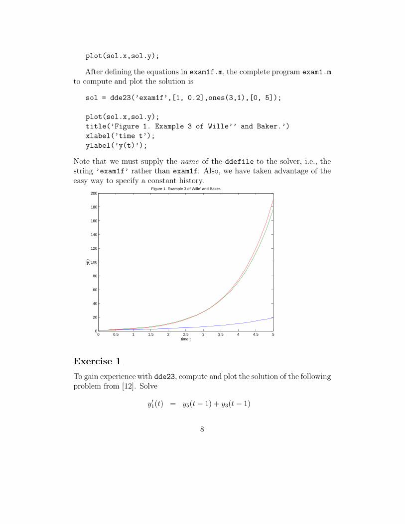
After defining the equations in exam1f.m, the complete program exam1.m
to compute and plot the solution is
sol = dde23(’exam1f’,[1, 0.2],ones(3,1),[0, 5]);
plot(sol.x,sol.y);
title(’Figure 1. Example 3 of Wille’’ and Baker.’)
xlabel(’time t’);
ylabel(’y(t)’);
Note that we must supply the name of the ddefile to the solver, i.e., thestring ’exam1f’ rather than exam1f. Also, we have taken advantage of theeasy way to specify a constant history.
0 0.5 1 1.5 2 2.5 3 3.5 4 4.5 50
20
40
60
80
100
120
140
160
180
200Figure 1. Example 3 of Wille’ and Baker.
time t
y(t)
Exercise 1
To gain experience with dde23, compute and plot the solution of the followingproblem from [12]. Solve
y′1(t) = y5(t− 1) + y3(t− 1)
8
y′2(t) = y1(t− 1) + y2(t− 0.5)
y′3(t) = y3(t− 1) + y1(t− 0.5)
y′4(t) = y5(t− 1)y4(t− 1)
y′5(t) = y1(t− 1)
on [0, 1] with history y1(t) = exp (t + 1), y2(t) = exp (t + 0.5), y3(t) = sin(t+1), y4(t) = y1(t), y5(t) = y1(t) for t ≤ 0.
In this you will have to evaluate the history in a function and supplyits name, say ’exer1h’, as the history argument of dde23. Remember thatboth the ddefile and the history function must return column vectors. In[12] this problem is used to show how to prepare a class of DDEs for solutionwith DMRODE. You might find it interesting to compare this preparationto what you had to do.
Example 2
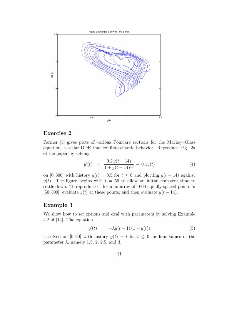
We show how to get output at specific points with Example 5 of [23], a scalarequation that exhibits chaotic behavior. We solve the equation
y′(t) =2 y(t− 2)
1 + y(t− 2)9.65− y(t) (3)
on [0, 100] with history y(t) = 0.5 for t ≤ 0.Output from dde23 is not just formally different from that of ode23.
dde23 computes an approximate solution S(t) valid throughout tspan andplaces in sol the information necessary to evaluate it. This evaluation isdone with ddeval. All you have to do is supply the solution structure andan array t of points where you want the values of S(t) and optionally S ′(t):
[S,Sp] = ddeval(sol,t);
With this form of output, you can solve a DDE just once and then obtaininexpensively as many solution values as you like, anywhere you like. Thenumerical solution itself is continuous and has a continuous derivative, soyou can always get a smooth graph by evaluating it at enough points withddeval.
The example of [23] plots y(t− 2) against y(t). This is quite a commontask in nonlinear dynamics, but we cannot proceed as in Example 1. That isbecause the entries of sol.x are not equally spaced: If t∗ appears in sol.x, we
9
have an approximation to y(t∗) in sol.y, but generally t∗−2 does not appearin sol.x, so we do not have an approximation to y(t∗ − 2). ddeval makessuch plots easy. In exam2.m we first define an array t of 1000 equally spacedpoints in [2, 100] and obtain solution values at these points with ddeval.We then use ddeval a second time to evaluate the solution at the entriesof t-2. In this way we obtain values approximating both y(t) and y(t − 2)for the same t. This might seem like a lot of plot points, but ddeval is justevaluating a piecewise-polynomial function and is coded to take advantage offast builtin functions and vectorization, so this is not expensive and resultsin a smooth graph.
Because Matlab does not distinguish scalars and vectors of one compo-nent, the single DDE can be coded as
function v = exam2f(t,y,Z)
v = 2*Z/(1 + Z^9.65) - y;
The complete program exam2.m to compute and plot y(t− 2) against y(t) is
sol = dde23(’exam2f’,2,0.5,[0, 100]);
t = linspace(2,100,1000);
y = ddeval(sol,t);
ylag = ddeval(sol,t - 2);
plot(y,ylag);
title(’Figure 2. Example 5 of Wille’’ and Baker.’)
xlabel(’y(t)’);
ylabel(’y(t-2)’);
axis([0 1.5 0 1.5])
10
0 0.5 1 1.50
0.5
1
1.5Figure 2. Example 5 of Wille’ and Baker.
y(t)
y(t−
2)
Exercise 2
Farmer [5] gives plots of various Poincare sections for the Mackey–Glassequation, a scalar DDE that exhibits chaotic behavior. Reproduce Fig. 2aof the paper by solving
y′(t) =0.2 y(t− 14)
1 + y(t− 14)10− 0.1y(t) (4)
on [0, 300] with history y(t) = 0.5 for t ≤ 0 and plotting y(t − 14) againsty(t). The figure begins with t = 50 to allow an initial transient time tosettle down. To reproduce it, form an array of 1000 equally spaced points in[50, 300], evaluate y(t) at these points, and then evaluate y(t− 14).
Example 3
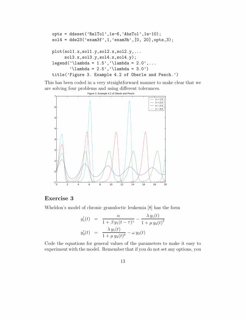
We show how to set options and deal with parameters by solving Example4.2 of [14]. The equation
y′(t) = −λy(t− 1) (1 + y(t)) (5)
is solved on [0, 20] with history y(t) = t for t ≤ 0 for four values of theparameter λ, namely 1.5, 2, 2.5, and 3.
11
Often default error tolerances are perfectly satisfactory, but here morestringent tolerances are needed for the larger values of λ. Options are setwith ddeset exactly as they are set for ode23 with odeset. When optionsare used, a call to dde23 has the form
sol = dde23(ddefile,lags,history,tspan,options);
Options like relative and absolute error tolerances are the same in the twosolvers. In particular, both have a default relative error tolerance of 10−3
and default absolute error tolerance of 10−6. The tolerances imposed for thelarger λ in exam3.m are relatively stringent for this solver, but this is a pricethat must be paid to obtain a satisfactory solution. To see this for yourself,try solving the problem with λ = 3 and default tolerances.
Parameters can always be communicated as global variables, but as iscommon with Matlab solvers, they can also be passed through dde23 asarguments following the options argument. For two values of λ we usedefault tolerances, so must use an empty array, [], as a placeholder for theoptions argument. When parameters are passed through dde23, they mustappear as arguments of the ddefile and if present, the history function, evenif they are not used. Accordingly, exam3f.m can be coded as
function v = exam3f(t,y,Z,lambda)
v = -lambda*Z*(1 + y);
and exam3h.m as
function v = exam3h(t,lambda)
v = t;
After defining the equation in exam3f.m and the history in exam3h.m, thecomplete program exam3.m to compute and plot the four solutions as in [14]is
title(’Figure 3. Example 4.2 of Oberle and Pesch.’)
This has been coded in a very straightforward manner to make clear that weare solving four problems and using different tolerances.
0 2 4 6 8 10 12 14 16 18 20−1
0
1
2
3
4
5
6
7Figure 3. Example 4.2 of Oberle and Pesch.
λ = 1.5λ = 2.0λ = 2.5λ = 3.0
Exercise 3
Wheldon’s model of chronic granuloctic leukemia [8] has the form
y′1(t) =α
1 + β y1(t− τ )γ− λ y1(t)
1 + µ y2(t)δ
y′2(t) =λ y1(t)
1 + µ y2(t)δ− ω y2(t)
Code the equations for general values of the parameters to make it easy toexperiment with the model. Remember that if you do not set any options, you
13
must use a placeholder of [] for the options argument. Solve the problem on[0, 200] with history y1(t) = 100, y2(t) = 100 for t ≤ 0 and parameter valuesα = 1.1 × 10¹⁰, β = 10−12, γ = 1.25, δ = 1, λ = 10, µ = 4 × 10⁻⁸, ω = 2.43that you set in the main program. Compare the solutions you obtain withτ = 7 and τ = 20. You could code this as
for tau = [7, 20]
sol = dde23(’exer3f’,tau,...
...
end
You should find that the solution is oscillatory in both cases. In the first,the oscillations are damped quickly and in the second, they are not.
Example 4
It is often necessary to find when a solution satisfies a certain relation, e.g.,when a component has a specific value. An event is said to occur when afunction of the solution, g(t, y(t), y(t − τ1), . . . , y(t − τk)), vanishes. Someproblems involve many of these “event functions”. This example shows howto use the powerful event location capability of dde23.
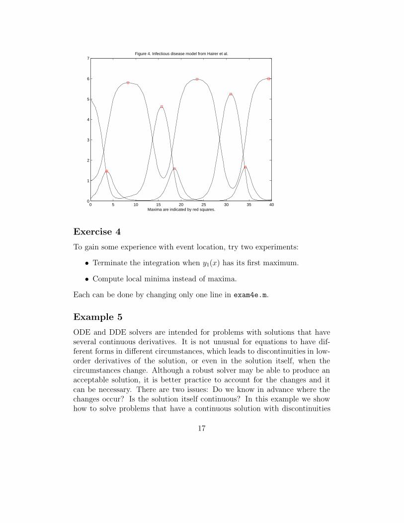
Figure 15.6 of [6] displays the solution of an infectious disease model. Theequations
y′1(x) = −y1(x)y2(x− 1) + y2(x− 10)
y′2(x) = y1(x)y2(x− 1) − y2(x)
y′3(x) = y2(x) − y2(x− 10)
are solved on [0, 40] with history y1(x) = 5, y2(x) = 0.1, y3(x) = 1 for x ≤ 0.To illustrate event location, we compute the local maxima of all three solutioncomponents.
We compute the maxima by finding where the first derivatives vanish.The three event functions come from the DDEs: y′1(x) = −y1(x)y2(x −1) + y2(x − 10), and so forth. All event functions are evaluated in a singleMatlab function that returns the values as a column vector. The name ofthis function is passed to the solver as the value of the ’Events’ option. Forthis example we evaluate the three functions in exam4e by a call to exam4f.Because event location is used for a variety of purposes, we have to tell dde23more about what we want to do. Sometimes we just want to know that an
14
event has occurred and other times we want to terminate the integrationthen. We tell the solver about this by returning a vector isterminal fromexam4e. To terminate the integration when event function k vanishes, weset component k of isterminal to 1 (true), and otherwise to 0 (false). Forthis example none of the events is terminal. There is an annoying matter ofsome importance: Sometimes we want to start an integration with an eventfunction that vanishes at the initial point. Imagine, for example, that we firea model rocket into the air and we want to know when it hits the ground. Itis natural to use the height of the rocket as a terminal event function, but itvanishes at the initial time as well as the final time. dde23 treats an eventat the initial point in a special way. The solver locates such an event andreports it, but does not treat it as terminal, no matter how isterminal is set.The example shows that how an event function vanishes may be important:To distinguish maxima from minima, we want the solver to report that aderivative vanished only when it changes from positive to negative values.This is done using direction. If we are interested only in events for whichevent function k is increasing through 0, we set component k of direction
to +1. Correspondingly, we set it to −1 if we are interested only in thoseevents for which the event function is decreasing, and 0 if we are interestedin all events. Once we understand what information must be provided, it iseasy to code the event functions of this example as
function [value,isterminal,direction] = exam4e(x,y,Z)
value = exam4f(x,y,Z);
isterminal = zeros(3,1);
direction = -ones(3,1);
Now that we have discussed how to tell the solver what we want it to do,we have to discuss how it reports what happened. The locations of eventsare returned as the field sol.xe and the values of the solution at these pointsare returned as the field sol.ye. If there are no events, sol.xe = []. Thefield sol.ie reports which event occurred. A value of k indicates that eventfunction k vanished at the corresponding entry of sol.xe.
It is straightforward to code the equations as
function v = exam4f(x,y,Z)
ylag1 = Z(:,1);
ylag2 = Z(:,2);
v = zeros(3,1);
15
v(1) = -y(1)*ylag1(2) + ylag2(2);
v(2) = y(1)*ylag1(2) - y(2);
v(3) = y(2) - ylag2(2);
With exam4e.m and exam4f, it is also straightforward to code the solutionof the problem as the first two lines of the complete solution exam4.m thatfollows:
options = ddeset(’Events’,’exam4e’);
sol = dde23(’exam4f’,[1, 10],[5; 0.1; 1],[0, 40],options);
title(’Figure 4. Infectious disease model from Hairer et al.’)
xlabel(’Maxima are indicated by red squares.’)
The only complication in this program is separating the various kinds ofevents. It is not necessary, but perhaps clearer, to introduce local variablesfor the fields that return the results of the event location. The command n1
= find(ie == 1) finds the indices corresponding to the first event function.These indices allow us to extract the information that y1(x) has its maximaat xe(n1) and its values there are ye(1,n1). The second and third eventfunctions are handled in the same way and then all the results are plotted.
16
0 5 10 15 20 25 30 35 400
1
2
3
4
5
6
7Figure 4. Infectious disease model from Hairer et al.
Maxima are indicated by red squares.
Exercise 4
To gain some experience with event location, try two experiments:
• Terminate the integration when y1(x) has its first maximum.
• Compute local minima instead of maxima.
Each can be done by changing only one line in exam4e.m.
Example 5
ODE and DDE solvers are intended for problems with solutions that haveseveral continuous derivatives. It is not unusual for equations to have dif-ferent forms in different circumstances, which leads to discontinuities in low-order derivatives of the solution, or even in the solution itself, when thecircumstances change. Although a robust solver may be able to produce anacceptable solution, it is better practice to account for the changes and itcan be necessary. There are two issues: Do we know in advance where thechanges occur? Is the solution itself continuous? In this example we showhow to solve problems that have a continuous solution with discontinuities
17
in a low-order derivative at points known in advance. The history is thesolution prior to the initial point and its discontinuities must also be takeninto account because they propagate into the interval of integration. Discon-tinuities in the history are handled in the same way, but are a little simplerbecause discontinuities in the history itself are permitted.
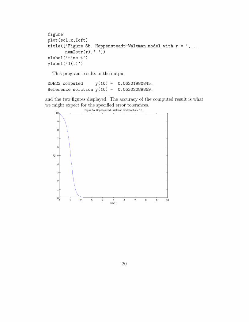
Example 4.4 of [14] is an infection model due to Hoppensteadt and Walt-man. The equation
y′(t) =
−r y(t) 0.4 (1 − t) if 0 ≤ t ≤ 1 − c,−r y(t) (0.4(1 − t) + 10 − eµy(t)) if 1 − c < t ≤ 1,−r y(t) (10 − eµy(t)) if 1 < t ≤ 2 − c,−r eµ y(t) (y(t− 1) − y(t)) if 2 − c < t.
is solved on [0, 10] with history y(t) = 10 for t ≤ 0. Here c = 1/√
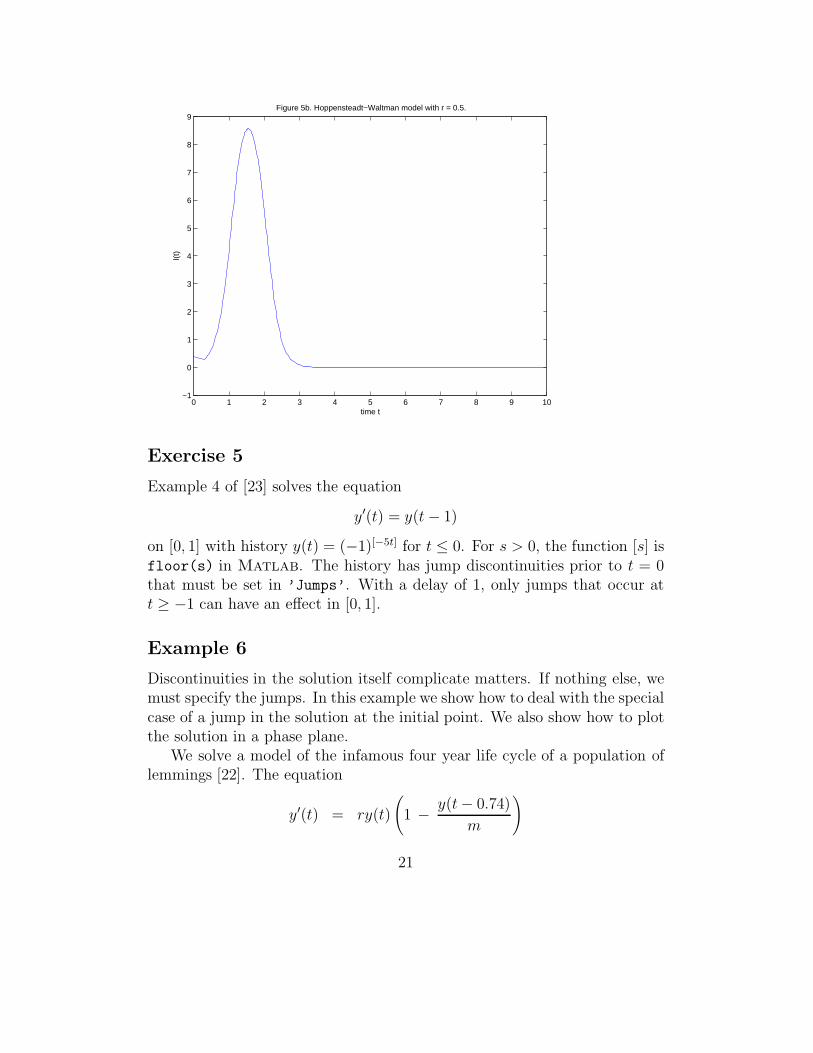
2 andµ = r/10. Oberle and Pesch solve this problem for several values of theparameter r, but we solve it only for r = 0.5. The different phases of thespread of the disease are described by different equations. In this example thephases change at times known in advance. The model requires the solutionto be continuous, but the changes in the equation lead to jumps in low orderderivatives. In addition to y(t), an approximation to I(t) = −y′(t)/(r y(t))is required.
dde23 deals easily with problems that have a continuous solution anddiscontinuities in low-order derivatives at known points. All you have to dois tell the solver where the discontinuities are by providing them as the valueof the ’Jumps’ option. However, you need to keep in mind that the historyis the solution prior to the initial point, so you must also account for itsdiscontinuities. For instance, the Marchuk immunology model discussed in[6, pp. 297–298] has the history max(0, t+ 10−6) for t ≤ 0. Its solution has ajump in the first derivative at t = −10−6 which propagates into the intervalof integration. Discontinuities in the history are handled like discontinuitiesat known points during the integration. In one respect they are simpler; ajump in the history itself is treated the same as a jump in one of its loworder derivatives. Low-order discontinuities in the history have an effect inthe interval of integration because of the delays. If the initial point is a andthe longest delay is T , discontinuities that occur before a− T have no effecton the integration, so there is no need to include them in ’Jumps’.
Having discussed how to deal with the discontinuities, it is straightforwardto solve the problem. We compute an approximation to y(10) and compare
18
it to an accurate value reported in [14]. This illustrates the computationof an approximation at a specific point and confirms the accuracy of thecomputation. We compute and plot I(t) at the points of sol.x using thefields sol.y and sol.yp. If we should want values at other t or should want asmoother graph, we would compute the necessary values with ddeval. If wetreat r as a parameter, the equation can be coded as
title([’Figure 5a. Hoppensteadt-Waltman model with r = ’,...
num2str(r),’.’])
xlabel(’time t’)
ylabel(’y(t)’)
Ioft = -(1/r)*(sol.yp ./ sol.y);
19
figure
plot(sol.x,Ioft)
title([’Figure 5b. Hoppensteadt-Waltman model with r = ’,...
num2str(r),’.’])
xlabel(’time t’)
ylabel(’I(t)’)
This program results in the output
DDE23 computed y(10) = 0.06301980845.
Reference solution y(10) = 0.06302089869.
and the two figures displayed. The accuracy of the computed result is whatwe might expect for the specified error tolerances.
0 1 2 3 4 5 6 7 8 9 100
1
2
3
4
5
6
7
8
9
10Figure 5a. Hoppensteadt−Waltman model with r = 0.5.
time t
y(t)
20
0 1 2 3 4 5 6 7 8 9 10−1
0
1
2
3
4
5
6
7
8
9Figure 5b. Hoppensteadt−Waltman model with r = 0.5.
time t
I(t)
Exercise 5
Example 4 of [23] solves the equation
y′(t) = y(t− 1)
on [0, 1] with history y(t) = (−1)[−5t] for t ≤ 0. For s > 0, the function [s] isfloor(s) in Matlab. The history has jump discontinuities prior to t = 0that must be set in ’Jumps’. With a delay of 1, only jumps that occur att ≥ −1 can have an effect in [0, 1].
Example 6
Discontinuities in the solution itself complicate matters. If nothing else, wemust specify the jumps. In this example we show how to deal with the specialcase of a jump in the solution at the initial point. We also show how to plotthe solution in a phase plane.
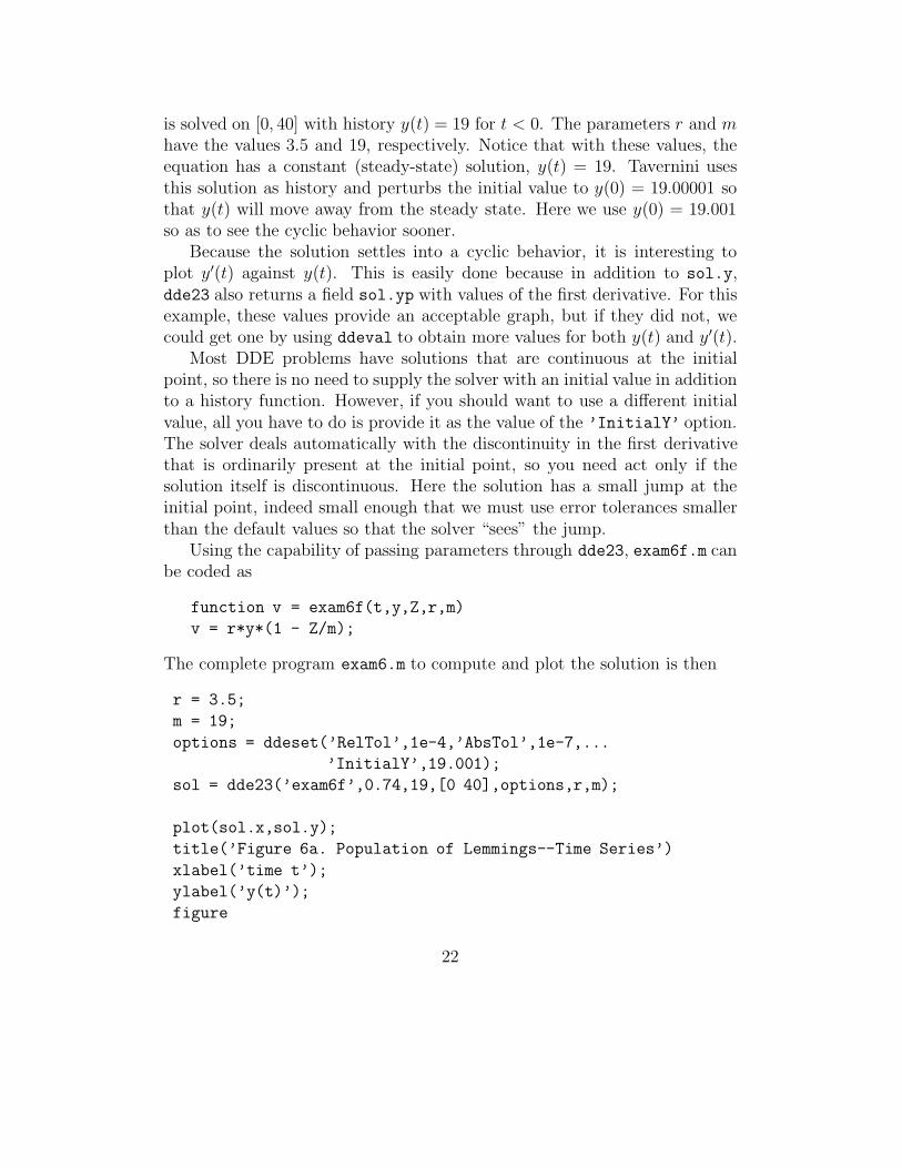
We solve a model of the infamous four year life cycle of a population oflemmings [22]. The equation
y′(t) = ry(t)
(1 − y(t− 0.74)
m
)
21
is solved on [0, 40] with history y(t) = 19 for t < 0. The parameters r and mhave the values 3.5 and 19, respectively. Notice that with these values, theequation has a constant (steady-state) solution, y(t) = 19. Tavernini usesthis solution as history and perturbs the initial value to y(0) = 19.00001 sothat y(t) will move away from the steady state. Here we use y(0) = 19.001so as to see the cyclic behavior sooner.
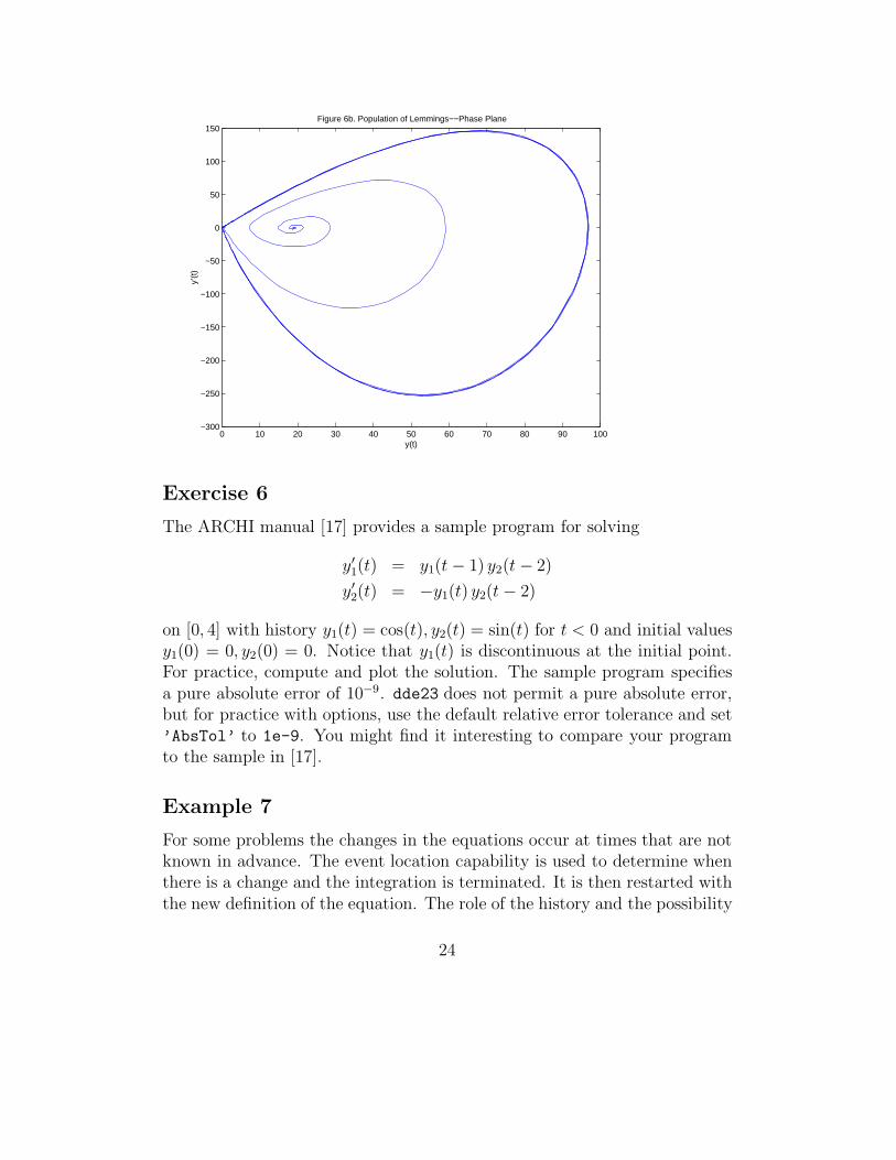
Because the solution settles into a cyclic behavior, it is interesting toplot y′(t) against y(t). This is easily done because in addition to sol.y,dde23 also returns a field sol.yp with values of the first derivative. For thisexample, these values provide an acceptable graph, but if they did not, wecould get one by using ddeval to obtain more values for both y(t) and y′(t).
Most DDE problems have solutions that are continuous at the initialpoint, so there is no need to supply the solver with an initial value in additionto a history function. However, if you should want to use a different initialvalue, all you have to do is provide it as the value of the ’InitialY’ option.The solver deals automatically with the discontinuity in the first derivativethat is ordinarily present at the initial point, so you need act only if thesolution itself is discontinuous. Here the solution has a small jump at theinitial point, indeed small enough that we must use error tolerances smallerthan the default values so that the solver “sees” the jump.
Using the capability of passing parameters through dde23, exam6f.m canbe coded as
function v = exam6f(t,y,Z,r,m)
v = r*y*(1 - Z/m);
The complete program exam6.m to compute and plot the solution is then
r = 3.5;
m = 19;
options = ddeset(’RelTol’,1e-4,’AbsTol’,1e-7,...
’InitialY’,19.001);
sol = dde23(’exam6f’,0.74,19,[0 40],options,r,m);
plot(sol.x,sol.y);
title(’Figure 6a. Population of Lemmings--Time Series’)
xlabel(’time t’);
ylabel(’y(t)’);
figure
22
plot(sol.y,sol.yp);
title(’Figure 6b. Population of Lemmings--Phase Plane’)
xlabel(’y(t)’);
ylabel(’y’’(t)’);
0 5 10 15 20 25 30 35 400
10
20
30
40
50
60
70
80
90
100Figure 6a. Population of Lemmings−−Time Series
time t
y(t)
Clearly the normalized population gets quite small, but how small? Areasonably accurate answer is obtained easily: The smallest value of y(t) isapproximately min(sol.y), namely 0.0116. If we wanted a better answer,we could obtain it by introducing event functions as in the last example.
23
0 10 20 30 40 50 60 70 80 90 100−300
−250
−200
−150
−100
−50
0
50
100
150Figure 6b. Population of Lemmings−−Phase Plane
y(t)
y’(t
)
Exercise 6
The ARCHI manual [17] provides a sample program for solving
y′1(t) = y1(t− 1) y2(t− 2)
y′2(t) = −y1(t) y2(t− 2)
on [0, 4] with history y1(t) = cos(t), y2(t) = sin(t) for t < 0 and initial valuesy1(0) = 0, y2(0) = 0. Notice that y1(t) is discontinuous at the initial point.For practice, compute and plot the solution. The sample program specifiesa pure absolute error of 10−9. dde23 does not permit a pure absolute error,but for practice with options, use the default relative error tolerance and set’AbsTol’ to 1e-9. You might find it interesting to compare your programto the sample in [17].
Example 7
For some problems the changes in the equations occur at times that are notknown in advance. The event location capability is used to determine whenthere is a change and the integration is terminated. It is then restarted withthe new definition of the equation. The role of the history and the possibility
24
of a jump discontinuity in the solution itself complicate this, but dde23 wasdesigned to make it as painless as possible. This example and the next showhow to proceed.
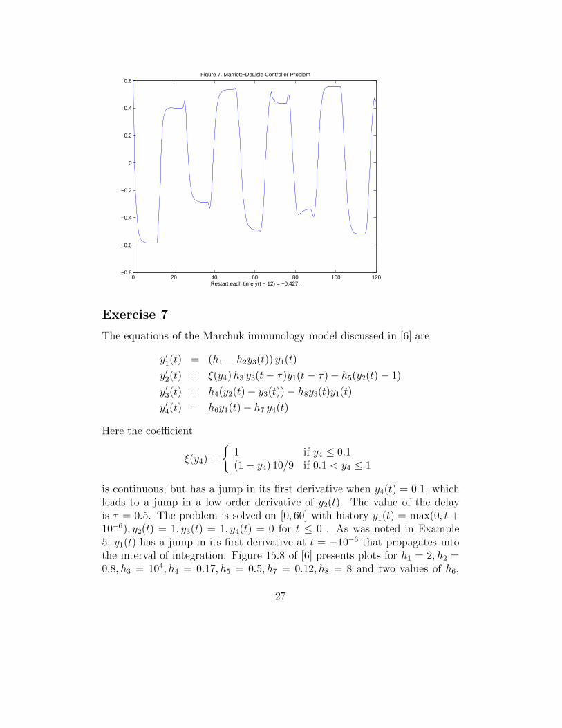
Marriott and DeLisle [10] solve a DDE that involves a step function ofthe history term. With ∆ = y(t− 12) − xb, the equation is
y′(t) =(−y(t) + π
(a + ε sign(∆) − u sin2(∆)
))/τ.
It is solved on [0, 120] with history y(t) = 0.6 for t ≤ 0 and parameter valuesxb = −0.427, a = 0.16, ε = 0.02, u = 0.5, τ = 1.
The term sign(∆) is an idealization of a sharp change that we do notexpect to resolve in detail. dde23 is sufficiently robust that it can solve thisproblem in a straightforward way. However, ignoring discontinuities can getyou into trouble even when solving an ODE [19], much less a DDE. You canbe much more confident of your numerical results if you arrange that thesolver is always integrating an equation with smooth coefficients. This canbe done here by letting the parameter state be the value the solver is touse for sign(∆). With the given history, it is initialized to +1. We integrateuntil the event function y(t−12)−xb vanishes. The ’Events’ option is usedto locate this event and terminate the integration then. The sign of state
is changed and the integration restarted. This continues until the end of theinterval is reached. It is straightforward to code the event location as
function [value,isterminal,direction] = exam7e(t,y,Z,state)
xb = -0.427;
value = Z - xb;
isterminal = 1;
direction = 0;
and with state defined in exam7.m as described, the evaluation of the DDEis coded as
function v = exam7f(t,y,Z,state)
xb = -0.427;
a = 0.16;
epsilon = 0.02;
u = 0.5;
tau = 1;
Delta = Z - xb;
v = (-y + pi * (a + epsilon*state - u*sin(Delta)^2)) / tau;
25
The event location capability deals with the issue of finding when theequations change, but there is a matter special to DDEs on restarting, thehistory. On a restart, dde23 accepts the previously computed solution struc-ture as history. dde23 updates the information in the solution structure eachtime it is called, so the solution returned is always valid from the initial to thelast point reached in the integration, namely sol.x(end). It is convenient tocompare this point to the end of the interval of integration and perform therestarts in a while loop. In this loop the solution structure of one integrationis used as the history for the next until the run is completed.
With exam7e.m and exam7f.m, the complete program exam7.m to com-pute and plot the solution is
state = +1;
opts = ddeset(’Events’,’exam7e’);
sol = dde23(’exam7f’,12,0.6,[0, 120],opts,state);
while sol.x(end) < 120
fprintf(’Restart at %5.1f.\n’,sol.x(end));
state = - state;
sol = dde23(’exam7f’,12,sol,[sol.x(end), 120],opts,state);
is continuous, but has a jump in its first derivative when y4(t) = 0.1, whichleads to a jump in a low order derivative of y2(t). The value of the delayis τ = 0.5. The problem is solved on [0, 60] with history y1(t) = max(0, t +10−6), y2(t) = 1, y3(t) = 1, y4(t) = 0 for t ≤ 0 . As was noted in Example5, y1(t) has a jump in its first derivative at t = −10−6 that propagates intothe interval of integration. Figure 15.8 of [6] presents plots for h1 = 2, h2 =0.8, h3 = 104, h4 = 0.17, h5 = 0.5, h7 = 0.12, h8 = 8 and two values of h6,
27
namely 10 and 300. Treat h6 as a parameter in your program and try toreproduce the figure for h6 = 300. For this you will have to plot the scaledcomponents 104y1, y2/2, y3, 10y4 with axis([0 60 -1 15.5]) . An arrayyplot of scaled values for plotting can be formed easily by
yplot = sol.y;
yplot(1,:) = 1e4*yplot(1,:);
and so forth. To solve this problem accurately over the whole interval, youwill need to reduce the tolerances to, say, a relative tolerance of 10−5 and anabsolute tolerance of 10−8.
dde23 is sufficiently robust that it can solve this problem in a straight-forward way. However, you can be much more confident of the results if youensure that the solver is always working with equations that have smoothcoefficients. There are two kinds of discontinuities in this problem. As inExample 5, use the ’Jumps’ option to tell the solver about the discontinu-ity at t = −10−6. As in Example 7, terminate the integration when theevent function y4(t) − 0.1 vanishes. Use a parameter state with value +1 ify4(t) ≤ 0.1 and −1 otherwise. The problem is to be solved with y4(0) = 0,so initialize state to +1. Thereafter, each time that the solver returns,check whether you have reached the end of the interval. If sol.x(end) <
60, change the sign of state and call dde23 again with the previous solutionas history. In the function for evaluating the DDEs, set ξ(y4) = 1 if state
is +1 and ξ(y4) = (1 − y4) 10/9 otherwise.
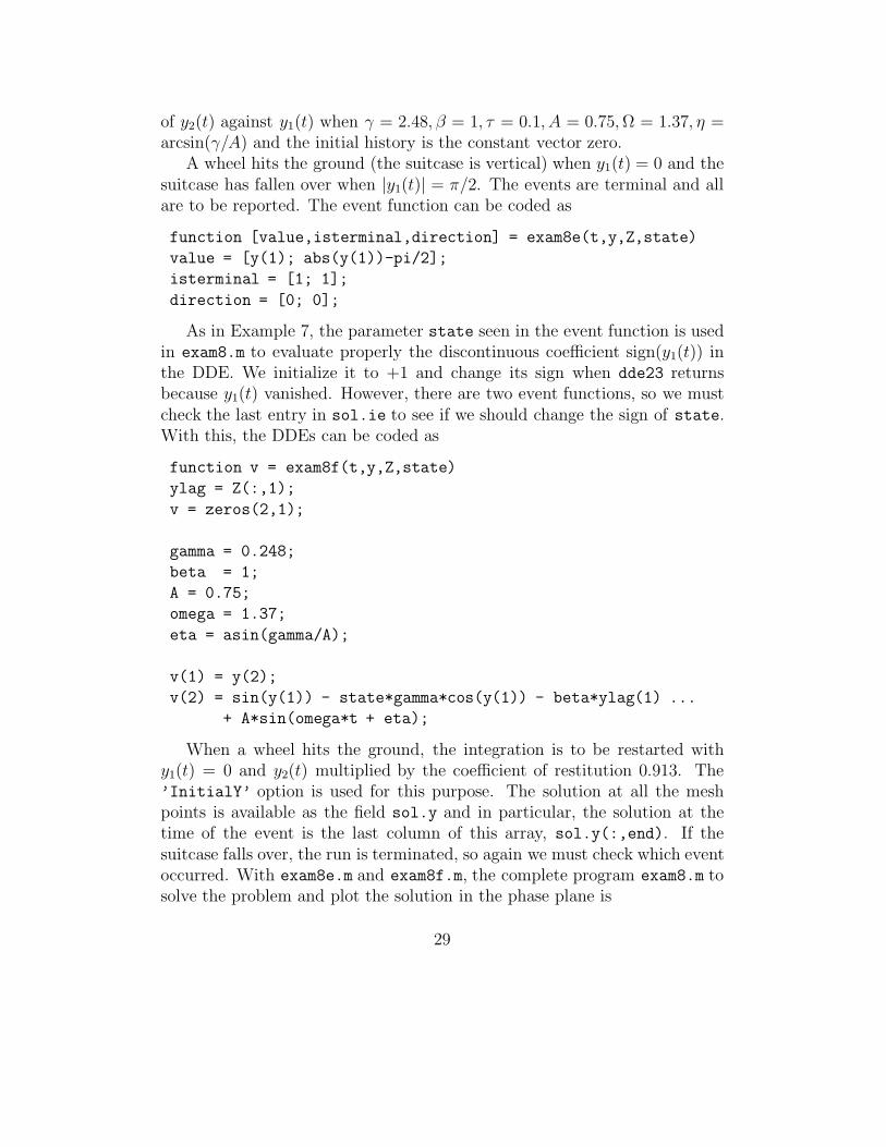
Example 8
This example is much like Example 7 except that the solution itself is dis-continuous. We restart at discontinuities, so the jump in the solution occursat the initial point of an integration and can be handled as in Example 6.
A two-wheeled suitcase may begin to rock from side to side as it is pulled.When this happens, the person pulling it attempts to return it to the verticalby applying a restoring moment to the handle. There is a delay in thisresponse that can affect significantly the stability of the motion. This ismodeled by Suherman et alia [21] with the DDE
The equation is solved on [0, 12] as a pair of first order equations with y1(t) =θ(t), y2(t) = θ′(t). Figure 3 of [21] shows a plot of y1(t) against t and a plot
28
of y2(t) against y1(t) when γ = 2.48, β = 1, τ = 0.1, A = 0.75,Ω = 1.37, η =arcsin(γ/A) and the initial history is the constant vector zero.
A wheel hits the ground (the suitcase is vertical) when y1(t) = 0 and thesuitcase has fallen over when |y1(t)| = π/2. The events are terminal and allare to be reported. The event function can be coded as
function [value,isterminal,direction] = exam8e(t,y,Z,state)
value = [y(1); abs(y(1))-pi/2];
isterminal = [1; 1];
direction = [0; 0];
As in Example 7, the parameter state seen in the event function is usedin exam8.m to evaluate properly the discontinuous coefficient sign(y1(t)) inthe DDE. We initialize it to +1 and change its sign when dde23 returnsbecause y1(t) vanished. However, there are two event functions, so we mustcheck the last entry in sol.ie to see if we should change the sign of state.With this, the DDEs can be coded as
When a wheel hits the ground, the integration is to be restarted withy1(t) = 0 and y2(t) multiplied by the coefficient of restitution 0.913. The’InitialY’ option is used for this purpose. The solution at all the meshpoints is available as the field sol.y and in particular, the solution at thetime of the event is the last column of this array, sol.y(:,end). If thesuitcase falls over, the run is terminated, so again we must check which eventoccurred. With exam8e.m and exam8f.m, the complete program exam8.m tosolve the problem and plot the solution in the phase plane is
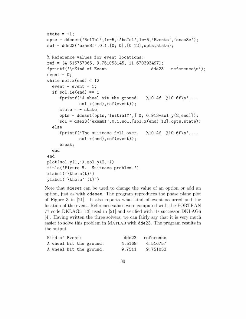
Note that ddeset can be used to change the value of an option or add anoption, just as with odeset. The program reproduces the phase plane plotof Figure 3 in [21]. It also reports what kind of event occurred and thelocation of the event. Reference values were computed with the FORTRAN77 code DKLAG5 [13] used in [21] and verified with its successor DKLAG6[4]. Having written the three solvers, we can fairly say that it is very mucheasier to solve this problem in Matlab with dde23. The program results inthe output
Kind of Event: dde23 reference
A wheel hit the ground. 4.5168 4.516757
A wheel hit the ground. 9.7511 9.751053
30
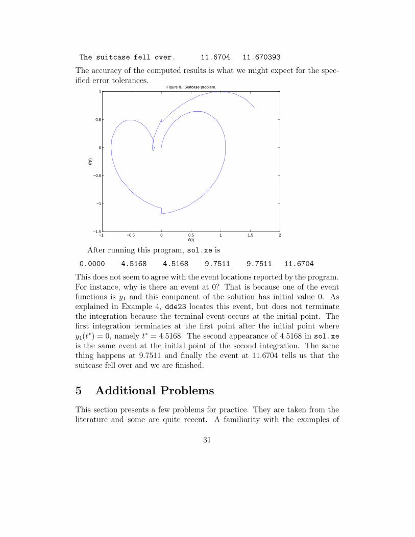
The suitcase fell over. 11.6704 11.670393
The accuracy of the computed results is what we might expect for the spec-ified error tolerances.
−1 −0.5 0 0.5 1 1.5 2−1.5
−1
−0.5
0
0.5
1Figure 8. Suitcase problem.
θ(t)
θ’(t
)
After running this program, sol.xe is
0.0000 4.5168 4.5168 9.7511 9.7511 11.6704
This does not seem to agree with the event locations reported by the program.For instance, why is there an event at 0? That is because one of the eventfunctions is y1 and this component of the solution has initial value 0. Asexplained in Example 4, dde23 locates this event, but does not terminatethe integration because the terminal event occurs at the initial point. Thefirst integration terminates at the first point after the initial point wherey1(t
∗) = 0, namely t∗ = 4.5168. The second appearance of 4.5168 in sol.xe
is the same event at the initial point of the second integration. The samething happens at 9.7511 and finally the event at 11.6704 tells us that thesuitcase fell over and we are finished.
5 Additional Problems
This section presents a few problems for practice. They are taken from theliterature and some are quite recent. A familiarity with the examples of
31
the previous section is assumed. Some hints are given and some output isprovided both as a check and to show how the solutions behave. Completesolutions are provided as additional templates. These problems and theirsolutions show that interesting problems can be solved easily in Matlabwith dde23.
Problem 1
Hale [7] cites predator–prey models obtained by introducing a resource lim-itation on the prey and assuming the birth rate of predators responds tochanges in the magnitude of the population y1 of prey and the populationy2 of predators only after a time delay τ . Starting with the system of ODEs[15]
y′1(t) = a y1(t) + b y1(t) y2(t)
y′2(t) = c y2(t) + d y1(t) y2(t)
we arrive in this way at a system of DDEs
y′1(t) = a y1(t)
(1 − y1(t)
m
)+ b y1(t) y2(t)
y′2(t) = c y2(t) + d y1(t− τ ) y2(t− τ )
It is interesting to explore the effect of the delay, so let us solve both systemson [0, 100] with initial value y1(0) = 80, y2(0) = 30 for the ODEs and thesame vector as constant history for the DDEs. Suppose that the parametersa = 0.25, b = −0.01, c = −1.00, d = 0.01, and m = 200.
Recall that you solve ODEs with dde23 by setting lags to []. Whenthis is done, the argument Z that dde23 supplies to the functions it calls isthe empty array. You can use this to code the evaluation of both sets ofequations in the same function by testing isempty(Z) to find out which setto evaluate. A more straightforward approach is to use two functions for thetwo sets of equations. Solve the DDE with τ = 1. Plot in one figure y2(t)against y1(t) for the two solutions. This phase plane plot of the solution ofthe ODEs should be a closed curve corresponding to a limit cycle. To achievethis you will need to tighten the error tolerances with a command like
opts = ddeset(’RelTol’,1e-5,’AbsTol’,1e-8);
32
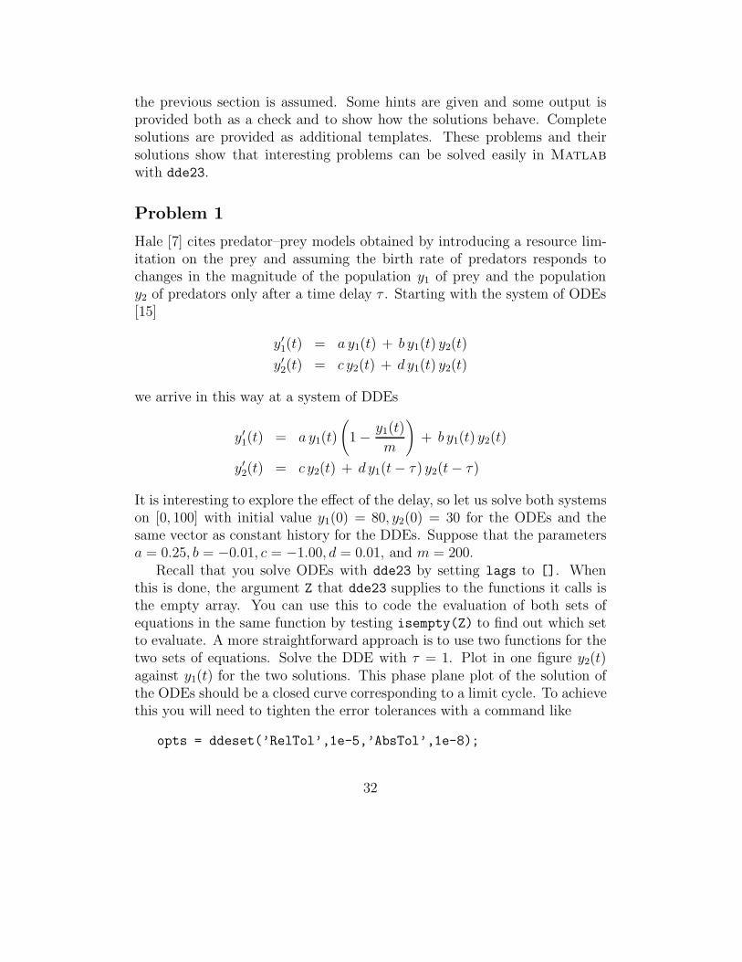
The figure makes the point that introducing a delay into an ODE model canhave a profound effect on the solution. If you experiment with τ , you willfind this to be true even for small delays. It is also interesting to remove theresource term 1 − y1(t)/m and see how the orbits change as τ is changed.
60 70 80 90 100 110 120 1305
10
15
20
25
30
35
40Problem 1. Solution with and without delay.
y1(t)
y 2(t)
No delayDelay τ = 1
Problem 2
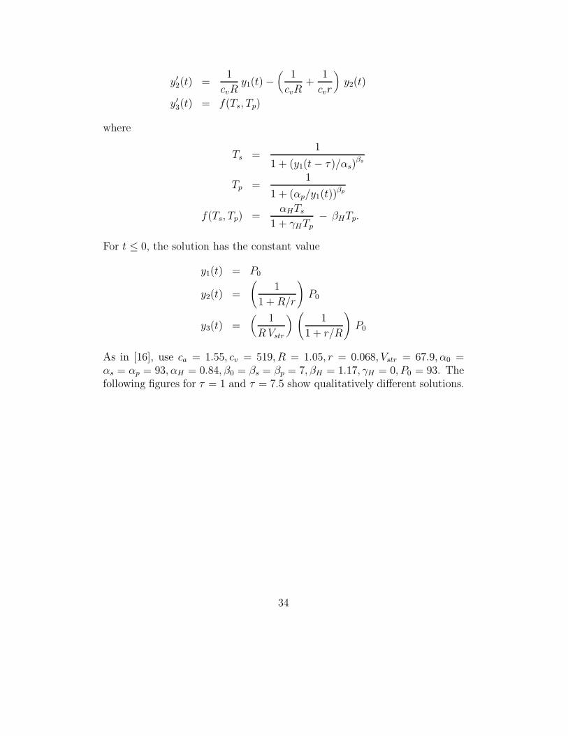
This problem considers a cardiovascular model due to Ottesen [16] involvingthe arterial pressure, Pa(t) = y1(t), the venous pressure, Pv(t) = y2(t), andthe heart rate, H(t) = y3(t). Ottesen studies conditions under which thedelay causes qualitative differences in the solution and in particular, oscil-lations in Pa(t). Delays τ = 1.0, 1.4, 3.9, 5.0, 7.5, 10 are considered in [16].There are a number of parameters in the model, so you might wish simplyto declare them as global values rather than pass them through dde23 tothe function for evaluating the equations, or even to hard code them. Ploty1(t) = Pa(t) for several values of τ . You should find that the solutionsobtained for different values of τ differ dramatically. Solve on [0, 350] theequations
y′1(t) = − 1
caRy1(t) +
1
caRy2(t) +
1
caVstr y3(t)
33
y′2(t) =1
cvRy1(t) −
(1
cvR+
1
cvr
)y2(t)
y′3(t) = f(Ts, Tp)
where
Ts =1
1 + (y1(t− τ )/αs)βs
Tp =1
1 + (αp/y1(t))βp
f(Ts, Tp) =αHTs
1 + γHTp
− βHTp.
For t ≤ 0, the solution has the constant value
y1(t) = P0
y2(t) =
(1
1 + R/r
)P0
y3(t) =(
1
RVstr
) (1
1 + r/R
)P0
As in [16], use ca = 1.55, cv = 519, R = 1.05, r = 0.068, Vstr = 67.9, α0 =αs = αp = 93, αH = 0.84, β0 = βs = βp = 7, βH = 1.17, γH = 0, P0 = 93. Thefollowing figures for τ = 1 and τ = 7.5 show qualitatively different solutions.
34
0 50 100 150 200 250 300 35082
84
86
88
90
92
94
96Problem 2. Baroflex Feedback Mechanism with τ = 1.
time t
Pa(t
)
0 50 100 150 200 250 300 35082
84
86
88
90
92
94
96Problem 2. Baroflex Feedback Mechanism with τ = 7.5.
time t
Pa(t
)
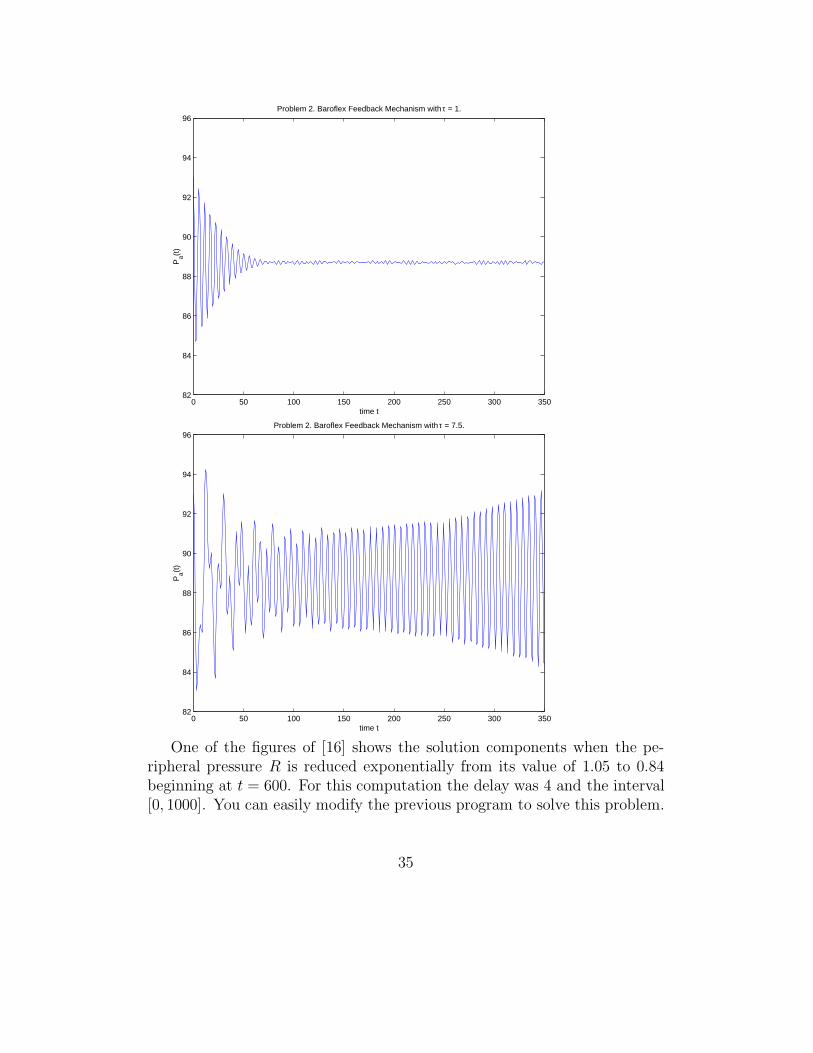
One of the figures of [16] shows the solution components when the pe-ripheral pressure R is reduced exponentially from its value of 1.05 to 0.84beginning at t = 600. For this computation the delay was 4 and the interval[0, 1000]. You can easily modify the previous program to solve this problem.
35
All you have to do is inform the solver of the low-order discontinuity at aknown time by setting the value of the ’Jumps’ option to 600, modify thefunction for evaluating the DDEs to include
if t <= 600
R = 1.05;
else
R = 0.21 * exp(600-t) + 0.84;
end
and use the specified delay and interval. All the solution components areof interest. The figure shows the sharp change in the heart rate due to thechange in R at t = 600.
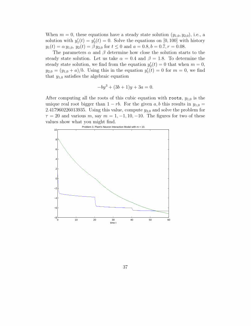
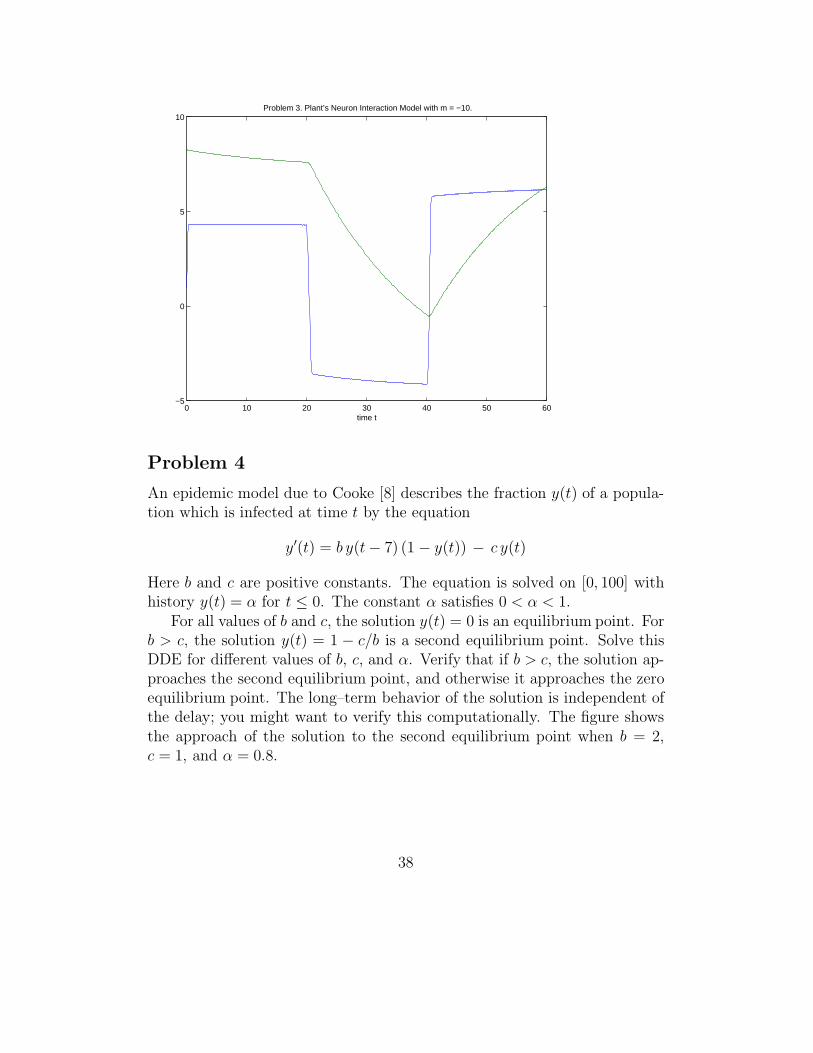
Plant’s Neuron Interaction Model [9] is given by the equations
y′1(t) = a y1(t) − y31(t)/3 + m (y1(t− τ ) − y1,0)
y′2(t) = r (y1(t) + a− b y2(t))
36
When m = 0, these equations have a steady state solution (y1,0, y2,0), i.e., asolution with y′1(t) = y′2(t) = 0. Solve the equations on [0, 100] with historyy1(t) = αy1,0, y2(t) = β y2,0 for t ≤ 0 and a = 0.8, b = 0.7, r = 0.08.
The parameters α and β determine how close the solution starts to thesteady state solution. Let us take α = 0.4 and β = 1.8. To determine thesteady state solution, we find from the equation y′2(t) = 0 that when m = 0,y2,0 = (y1,0 + a)/b. Using this in the equation y′1(t) = 0 for m = 0, we findthat y1,0 satisfies the algebraic equation
−by3 + (3b + 1)y + 3a = 0.
After computing all the roots of this cubic equation with roots, y1,0 is theunique real root bigger than 1 − rb. For the given a, b this results in y1,0 =2.417960226013935. Using this value, compute y2,0 and solve the problem forτ = 20 and various m, say m = 1,−1, 10,−10. The figures for two of thesevalues show what you might find.
0 10 20 30 40 50 60−8
−6
−4
−2
0
2
4
6
8
10Problem 3. Plant’s Neuron Interaction Model with m = 10.
time t
37
0 10 20 30 40 50 60−5
0
5
10Problem 3. Plant’s Neuron Interaction Model with m = −10.
time t
Problem 4
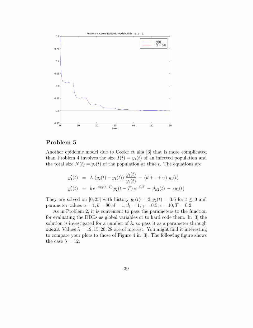
An epidemic model due to Cooke [8] describes the fraction y(t) of a popula-tion which is infected at time t by the equation
y′(t) = b y(t− 7) (1 − y(t)) − c y(t)
Here b and c are positive constants. The equation is solved on [0, 100] withhistory y(t) = α for t ≤ 0. The constant α satisfies 0 < α < 1.
For all values of b and c, the solution y(t) = 0 is an equilibrium point. Forb > c, the solution y(t) = 1 − c/b is a second equilibrium point. Solve thisDDE for different values of b, c, and α. Verify that if b > c, the solution ap-proaches the second equilibrium point, and otherwise it approaches the zeroequilibrium point. The long–term behavior of the solution is independent ofthe delay; you might want to verify this computationally. The figure showsthe approach of the solution to the second equilibrium point when b = 2,c = 1, and α = 0.8.
38
0 10 20 30 40 50 600.45
0.5
0.55
0.6
0.65
0.7
0.75
0.8Problem 4. Cooke Epidemic Model with b = 2 , c = 1.
time t
y(t)1 − c/b
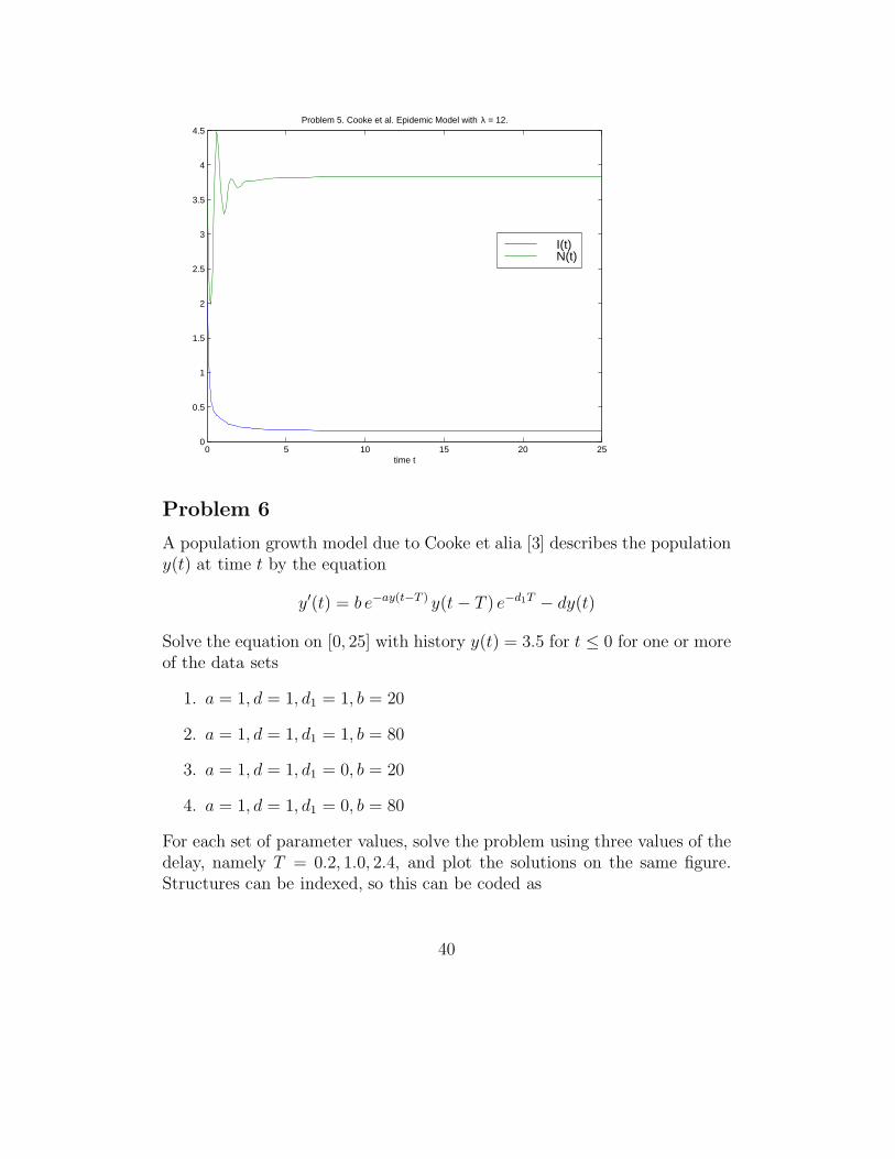
Problem 5
Another epidemic model due to Cooke et alia [3] that is more complicatedthan Problem 4 involves the size I(t) = y1(t) of an infected population andthe total size N(t) = y2(t) of the population at time t. The equations are
y′1(t) = λ (y2(t) − y1(t))y1(t)
y2(t)− (d + ε + γ) y1(t)
y′2(t) = b e−ay2(t−T ) y2(t− T ) e−d1T − dy2(t) − εy1(t)
They are solved on [0, 25] with history y1(t) = 2, y2(t) = 3.5 for t ≤ 0 andparameter values a = 1, b = 80, d = 1, d1 = 1, γ = 0.5, ε = 10, T = 0.2.
As in Problem 2, it is convenient to pass the parameters to the functionfor evaluating the DDEs as global variables or to hard code them. In [3] thesolution is investigated for a number of λ, so pass it as a parameter throughdde23. Values λ = 12, 15, 20, 28 are of interest. You might find it interestingto compare your plots to those of Figure 4 in [3]. The following figure showsthe case λ = 12.
39
0 5 10 15 20 250
0.5
1
1.5
2
2.5
3
3.5
4
4.5
time t
Problem 5. Cooke et al. Epidemic Model with λ = 12.
I(t)N(t)
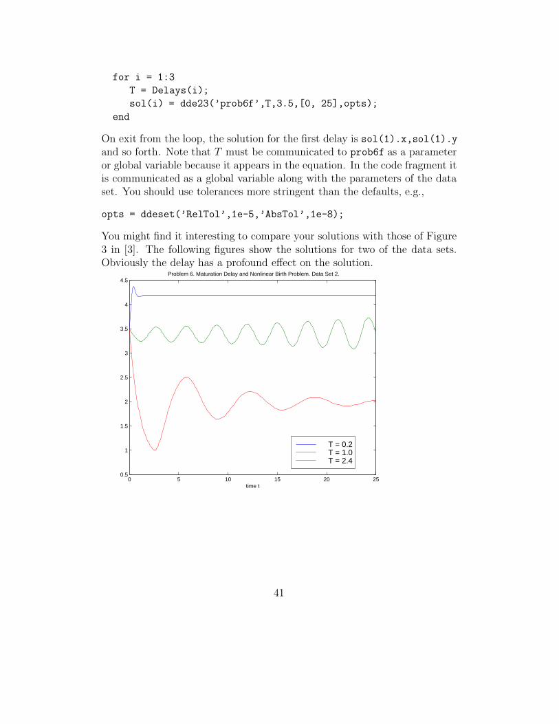
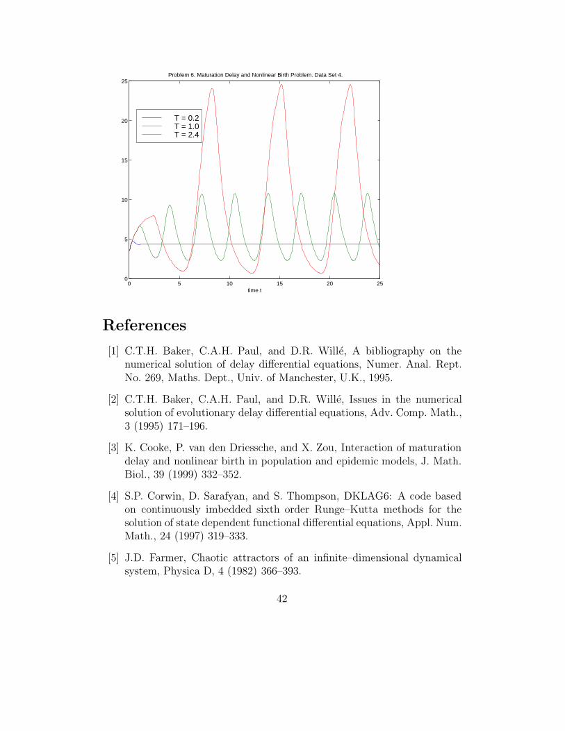
Problem 6
A population growth model due to Cooke et alia [3] describes the populationy(t) at time t by the equation
y′(t) = b e−ay(t−T ) y(t− T ) e−d1T − dy(t)
Solve the equation on [0, 25] with history y(t) = 3.5 for t ≤ 0 for one or moreof the data sets
1. a = 1, d = 1, d1 = 1, b = 20
2. a = 1, d = 1, d1 = 1, b = 80
3. a = 1, d = 1, d1 = 0, b = 20
4. a = 1, d = 1, d1 = 0, b = 80
For each set of parameter values, solve the problem using three values of thedelay, namely T = 0.2, 1.0, 2.4, and plot the solutions on the same figure.Structures can be indexed, so this can be coded as
40
for i = 1:3
T = Delays(i);
sol(i) = dde23(’prob6f’,T,3.5,[0, 25],opts);
end
On exit from the loop, the solution for the first delay is sol(1).x,sol(1).yand so forth. Note that T must be communicated to prob6f as a parameteror global variable because it appears in the equation. In the code fragment itis communicated as a global variable along with the parameters of the dataset. You should use tolerances more stringent than the defaults, e.g.,
opts = ddeset(’RelTol’,1e-5,’AbsTol’,1e-8);
You might find it interesting to compare your solutions with those of Figure3 in [3]. The following figures show the solutions for two of the data sets.Obviously the delay has a profound effect on the solution.
0 5 10 15 20 250.5
1
1.5
2
2.5
3
3.5
4
4.5
time t
Problem 6. Maturation Delay and Nonlinear Birth Problem. Data Set 2.
T = 0.2T = 1.0T = 2.4
41
0 5 10 15 20 250
5
10
15
20
25
time t
Problem 6. Maturation Delay and Nonlinear Birth Problem. Data Set 4.
T = 0.2T = 1.0T = 2.4
References
[1] C.T.H. Baker, C.A.H. Paul, and D.R. Wille, A bibliography on thenumerical solution of delay differential equations, Numer. Anal. Rept.No. 269, Maths. Dept., Univ. of Manchester, U.K., 1995.
[2] C.T.H. Baker, C.A.H. Paul, and D.R. Wille, Issues in the numericalsolution of evolutionary delay differential equations, Adv. Comp. Math.,3 (1995) 171–196.
[3] K. Cooke, P. van den Driessche, and X. Zou, Interaction of maturationdelay and nonlinear birth in population and epidemic models, J. Math.Biol., 39 (1999) 332–352.
[4] S.P. Corwin, D. Sarafyan, and S. Thompson, DKLAG6: A code basedon continuously imbedded sixth order Runge–Kutta methods for thesolution of state dependent functional differential equations, Appl. Num.Math., 24 (1997) 319–333.
[5] J.D. Farmer, Chaotic attractors of an infinite–dimensional dynamicalsystem, Physica D, 4 (1982) 366–393.
42
[6] E. Hairer, S.P. Nørsett, and G. Wanner, Solving Ordinary DifferentialEquations I, Springer-Verlag, Berlin, 1987.
[7] J. Hale, Functional Differential Equations, Springer-Verlag, Berlin, 1971.
[8] N. MacDonald, Time Lags in Biological Models, Springer-Verlag, Berlin,1978.
[9] N. MacDonald, Biological Delay Systems: Linear Stability Theory, Cam-bridge University Press, Cambridge, 1989.
[10] C. Marriott and C. DeLisle, Effects of discontinuities in the behavior ofa delay differential equation, Physica D, 36 (1989) 198–206.
[11] Matlab 5, The MathWorks, Inc., 3 Apple Hill Dr., Natick, MA 01760,1998.
[13] K.W. Neves and S. Thompson, Software for the numerical solution ofsystems of functional differential equations with state dependent delays,Appl. Num. Math., 9 (1992), 385–401.
[14] H.J. Oberle and H.J. Pesch, Numerical treatment of delay differentialequations by Hermite interpolation, Numer. Math., 37 (1981) 235–255.
[15] J.M. Ortega and W.G. Poole, An Introduction to Numerical Methodsfor Differential Equations, Pitman Publishing Inc., Marshfield, Mas-sachusetts, 1981.
[16] J.T. Ottesen, Modelling of the Baroflex–Feedback Mechanism WithTime–Delay, J. Math. Biol., 36 (1997), 41–63.
[17] C.A.H. Paul, A user-guide to Archi, Numer. Anal. Rept. No. 283, Maths.Dept., Univ. of Manchester, U.K., 1995.
[18] L.F. Shampine and M.W. Reichelt, The Matlab ODE suite, SIAM J.Sci. Comput., 18 (1997) 1–22.
[19] L.F. Shampine and S. Thompson, Event location for ordinary differentialequations, Comp. & Maths. with Appls., 39 (2000) 43–54.
43
[20] L.F. Shampine and S. Thompson, Solving DDEs in Matlab,manuscript.
[21] S. Suherman, R.H. Plaut, L.T. Watson, and S. Thompson, Effect ofhuman response time on rocking instability of a two–wheeled suitcase,J. of Sound and Vibration, 207 (1997) 617–625.
[22] L. Tavernini, Continuous–Time Modeling and Simulation, Gordon andBreach, Amsterdam, 1996.
[23] D.R. Wille and C.T.H. Baker, DELSOL – a numerical code for thesolution of systems of delay–differential equations, Appl. Numer. Math.,9 (1992) 223–234.