Solving differential equations with genetic programming I. G. Tsoulos, I. E. Lagaris * Department of Computer Science, University of Ioannina P.O. Box 1186, Ioannina 45110 - Greece Abstract A novel method for solving ordinary and partial differential equations, based on grammat- ical evolution is presented. The method forms generations of trial solutions expressed in an analytical closed form. Several examples are worked out and in most cases the exact solution is recovered. When the solution cannot be expressed in a closed analytical form then our method produces an approximation with a controlled level of accuracy. We report results on several problems to illustrate the potential of this approach. Keywords: Grammatical evolution, genetic programming, differential equations, evolutionary modeling. 1 Introduction A lot of problems in the fields of physics, chemistry, economics etc. can be expressed in terms of ordinary differential equations(ODE’s) and partial differential equations (PDE’s). Weather forecasting, quantum mechanics, wave propagation and stock market dynamics are some examples. For that reason many methods have been proposed for solving ODE’s and PDE’s such as Runge Kutta, Predictor - Corrector [1], radial basis functions [4] and feedforward neural networks [5]. Recently, methods based on genetic programming have also been proposed [6], as well as methods that induce the underlying differential equation from experimental data [7, 8]. The technique of genetic programming [2], is an optimization process based on the evolution of a large number of candidate solutions through genetic operations such as replication, crossover and mutation [14]. In this article we propose a novel method based on genetic programming. Our method attempts to solve ODE’s and PDE’s by generating solutions in a closed analytical form. Offering closed form analytical solutions is very helpful and highly desirable. Methods that offer such type of solutions have appeared in the past. We mention the Galerkin type of methods, methods based on neural networks [5], etc. These methods choose a basis set of functions with adjustable parameters and proceed approximating the solution by varying these parameters. Our method offers closed form solutions, however the variety of the basis functions involved is not a priori determined, rather is constructed dynamically as the solution procedure proceeds and can be of high complexity if required. This last feature is the one that distinguishes our method from others. We have not dealt with the problem of differential equation induction from data. The generation is achieved with the help of grammatical evolution. We used grammatical evolution instead the ”classic” tree based genetic programming, because grammatical evolution can produce programs in an arbitrary language, the genetic operations such as crossover and mutation are faster and also because it is far more convenient to symbolically differentiate mathematical expressions. The code production is performed using a mapping process governed by a grammar expressed in Backus Naur Form. Grammatical evolution has been applied successfully to problems such as symbolic regression [11], discovery of trigonometric identities [12], robot control [15], caching algorithms [16], financial prediction [17] etc. The rest of this article is organized as follows: in section 2 we give a brief * Corresponding author 1
Transcript
Solving differential equations with genetic programming
I. G. Tsoulos, I. E. Lagaris∗
Department of Computer Science, University of IoanninaP.O. Box 1186, Ioannina 45110 - Greece
Abstract
A novel method for solving ordinary and partial differential equations, based on grammat-
ical evolution is presented. The method forms generations of trial solutions expressed in an
analytical closed form. Several examples are worked out and in most cases the exact solution
is recovered. When the solution cannot be expressed in a closed analytical form then our
method produces an approximation with a controlled level of accuracy. We report results on
several problems to illustrate the potential of this approach.
A lot of problems in the fields of physics, chemistry, economics etc. can be expressed in termsof ordinary differential equations(ODE’s) and partial differential equations (PDE’s). Weatherforecasting, quantum mechanics, wave propagation and stock market dynamics are some examples.For that reason many methods have been proposed for solving ODE’s and PDE’s such as RungeKutta, Predictor - Corrector [1], radial basis functions [4] and feedforward neural networks [5].Recently, methods based on genetic programming have also been proposed [6], as well as methodsthat induce the underlying differential equation from experimental data [7, 8]. The technique ofgenetic programming [2], is an optimization process based on the evolution of a large number ofcandidate solutions through genetic operations such as replication, crossover and mutation [14]. Inthis article we propose a novel method based on genetic programming. Our method attempts tosolve ODE’s and PDE’s by generating solutions in a closed analytical form. Offering closed formanalytical solutions is very helpful and highly desirable. Methods that offer such type of solutionshave appeared in the past. We mention the Galerkin type of methods, methods based on neuralnetworks [5], etc. These methods choose a basis set of functions with adjustable parameters andproceed approximating the solution by varying these parameters. Our method offers closed formsolutions, however the variety of the basis functions involved is not a priori determined, ratheris constructed dynamically as the solution procedure proceeds and can be of high complexity ifrequired. This last feature is the one that distinguishes our method from others. We have notdealt with the problem of differential equation induction from data. The generation is achievedwith the help of grammatical evolution. We used grammatical evolution instead the ”classic” treebased genetic programming, because grammatical evolution can produce programs in an arbitrarylanguage, the genetic operations such as crossover and mutation are faster and also because it isfar more convenient to symbolically differentiate mathematical expressions. The code productionis performed using a mapping process governed by a grammar expressed in Backus Naur Form.Grammatical evolution has been applied successfully to problems such as symbolic regression [11],discovery of trigonometric identities [12], robot control [15], caching algorithms [16], financialprediction [17] etc. The rest of this article is organized as follows: in section 2 we give a brief
∗Corresponding author
1
presentation of grammatical evolution, in section 3 we describe in detail the new algorithm, insection 4 we present several experiments and in section 5 we present our conclusions and ideas forfurther work.
2 Grammatical Evolution
Grammatical evolution is an evolutionary algorithm that can produce code in any programminglanguage. The algorithm requires as inputs the BNF grammar definition of the target language andthe appropriate fitness function. Chromosomes in grammatical evolution, in contrast to classicalgenetic programming [2], are not expressed as parse trees, but as vectors of integers. Each integerdenotes a production rule from the BNF grammar. The algorithm starts from the start symbol ofthe grammar and gradually creates the program string, by replacing non terminal symbols withthe right hand of the selected production rule. The selection is performed in two steps:
• We read an element from the chromosome (with value V ).
• We select the rule according to the scheme
Rule = V mod NR (1)
where NR is the number of rules for the specific non-terminal symbol. The process of replacingnon terminal symbols with the right hand of production rules is continued until either a fullprogram has been generated or the end of chromosome has been reached. In the latter case wecan reject the entire chromosome or we can start over (wrapping event) from the first element ofthe chromosome. In our approach we allow at most two wrapping events to occur.
In our method we used a small part of the C programming language grammar as we can see infigure 1. The numbers in parentheses denote the sequence number of the corresponding productionrule to be used in the selection procedure described above.
2
Figure 1: The grammar of the proposed method
S::=<expr> (0)
<expr> ::= <expr> <op> <expr> (0)
| ( <expr> ) (1)
| <func> ( <expr> ) (2)
|<digit> (3)
|x (4)
|y (5)
|z (6)
<op> ::= + (0)
| - (1)
| * (2)
| / (3)
<func> ::= sin (0)
|cos (1)
|exp (2)
|log (3)
<digit> ::= 0 (0)
| 1 (1)
| 2 (2)
| 3 (3)
| 4 (4)
| 5 (5)
| 6 (6)
| 7 (7)
| 8 (8)
| 9 (9)
The symbol S in the grammar denotes the start symbol of the grammar. For example, suppose wehave the chromosome x = [16, 3, 7, 4, 10, 28, 24, 1, 2, 4]. In table 1 we show how a valid function isproduced from x. The resulting function in the above example is f(x) = log(x2). Further detailsabout grammatical evolution can be found in [9, 10, 11, 13]
log(x<op><expr>) 10, 28, 24, 1, 2, 4 10 mod 4 =2log(x*<expr>) 28, 24, 1, 2, 4 28 mod 7 =0
log(x*<expr><op><expr>) 24, 1, 2, 4 24 mod 7=3log(x*<digit><op><expr>) 1, 2, 4 1 mod 10=1
log(x*1<op><expr>) 2, 4 2 mod 4=2log(x*1*<expr>) 4 4 mod 7=4
log(x*1*x)
3
3 Description of the algorithm
To solve a given differential equation the proper boundary / initial conditions must be stated. Thealgorithm has the following phases:
1. Initialization.
2. Fitness evaluation.
3. Genetic operations.
4. Termination control.
3.1 Initialization
In the initialization phase the values for mutation rate and replication rate are set. The replicationrate denotes the fraction of the number of chromosomes that will go through unchanged to the nextgeneration(replication). That means that the probability for crossover is set to 1−replication rate.The mutation rate controls the average number of changes inside a chromosome.
3.2 Fitness evaluation
3.2.1 ODE case
We express the ODE’s in the following form:
f(
x, y, y(1), ..., y(n−1), y(n))
= 0, x ∈ [a, b] (2)
where y(n) denotes the n-order derivative of y. Let the boundary or initial conditions be given by:
gi
(
x, y, y(1), ..., y(n−1))
|x=ti
= 0, i = 1, ..., n
where ti is one of the two endpoints a or b. The steps for the fitness evaluation of the populationare the following:
1. Choose N equidistant points (x0, x1, ..., xN−1) in the relevant range.
2. For every chromosome i
(a) Construct the corresponding model Mi(x), expressed in the grammar described earlier.
(b) Calculate the quantity
E(Mi) =
N−1∑
j=0
(
f(
xj , M0i (xj), .., M
(n)i (xj)
))2
(3)
(c) Calculate an associated penalty P (Mi) as shown below.
(d) Calculate the fitness value of the chromosome as:
vi = E(Mi) + P (Mi) (4)
The penalty function P depends on the boundary conditions and it has the form:
P (Mi) = λ
n∑
k=1
g2k
(
x, Mi, M(1)i , ..., M
(n−1)i
)
|x=tk
(5)
where λ is a positive number.
4
3.2.2 SODE case
The proposed method can solve systems of ordinary differential equations that are expressed inthe form:
f1(x, y1, y(1)1 , y2, y
(1)2 , . . . , yk, y
(1)k ) = 0
f2(x, y1, y(1)1 , y2, y
(1)2 , . . . , yk, y
(1)k ) = 0
......
...
fk(x, y1, y(1)1 , y2, y
(1)2 , . . . , yk, y
(1)k ) = 0
, x ∈ [a, b] (6)
with initial conditions:
y1(a) = y1a
y2(a) = y2a
......
...yk(a) = yka
(7)
The steps for the fitness evaluation are the following:
1. Choose N equidistant points (x0, x1, ..., xN−1) in the relevant range.
2. For every chromosome i
(a) Split the chromosome uniformly in k parts, where k is the number of equations in thesystem.
(b) Construct the k models Mij , j = 1 . . . k
(c) Calculate the quantities
E(Mij) =
N−1∑
l=0
(
fj(xl, Mi1(xl), M(1)i1 (xl), Mi2(xl), M
(1)i2 (xl), . . . , Mik(xl), M
(1)ik (xl)
)2
,∀j = 1 . . . k
(d) Calculate the quantity
E(Mi) =k
∑
j=1
(E(Mij)) (8)
(e) Calculate the associated penalties
P (Mij) = λ (Mij(a) − yja)2 , ∀j = 1 . . . k (9)
where λ is a positive number.
(f) Calculate the total penalty value
P (Mi) =
k∑
j=1
(P (Mij)) (10)
(g) Finally, the fitness of the chromosome i is given by:
ui = E(Mi) + P (Mi) (11)
5
3.2.3 PDE case
We only consider here elliptic PDE’s in two and three variables with Dirichlet boundary conditions.The generalization of the process to other types of boundary conditions and higher dimensions isstraightforward. The PDE is expressed in the form:
f
(
x, y, Ψ(x, y),∂
∂xΨ(x, y),
∂
∂yΨ(x, y),
∂2
∂x2Ψ(x, y),
∂2
∂y2Ψ(x, y)
)
= 0 (12)
with x ∈ [x0, x1] and y ∈ [y0, y1]. The associated Dirichlet boundary conditions are expressedas: Ψ(x0, y) = f0(y), Ψ(x1, y) = f1(y), Ψ(x, y0) = g0(x), Ψ(x, y1) = g1(x).
The steps for the fitness evaluation of the population are given below:
1. Choose N2 equidistant points in the box [x0, x1] × [y0, y1], Nx equidistant points on theboundary at x = x0 and at x = x1, Ny equidistant points on the boundary at y = y0 and aty = y1.
2. For every chromosome i
• Construct a trial solution Mi(x, y) expressed in the grammar described earlier.
with the boundary conditions y(0) = 0 and y′(0) = 10. We take in the range [0, 1] N = 10 equidis-tant points x0, . . . , x9. Suppose that we have chromosomes with length 10 and one chromosome isthe array: g = [7, 2, 10, 4, 4, 2, 11, 20, 30, 5]. The function which corresponds to the chromosome g
is Mg(x) = exp(x)+sin(x). The first order derivative is M(1)(x)g = exp(x)+cos(x) and the second
6
order derivative is M(2)(x)g = exp(x) − sin(x). The symbolic computation of the above quantities
is described in detail in the section 2. Using the equation 3 we have:
E(Mg) =
9∑
i=0
(
M (2)g (xi) + 100Mg(xi)
)2
=
9∑
i=0
(101 exp(xi) + 99 sin(xi))2
= 4849332.4
The penalty function P (Mg) is calculated following the equation 5 as:
So, the fitness value ug of the chromosome is given by:
ug = E(Mg) + P (Mg)
= 4849332.4 + 82λ
We perform the above procedure to all chromosomes in the population and we sort them inascending order according to their fitness value. In consequence, we apply the genetic operators,the new population is created and the process is repeated until the termination criteria are met.
3.3 Evaluation of derivatives
Derivatives are evaluated together with the corresponding functions using an additional stack andthe following differentiation elementary rules, adopted by the various Automatic DifferentiationMethods [21] and used in corresponding tools [18, 19, 20]:
1. (f(x) + g(x))′ = f ′(x) + g′(x)
2. (f(x)g(x))′ = f ′(x)g(x) + f(x)g′(x)
3.(
f(x)g(x)
)′
= f ′(x)g(x)−g′(x)f(x)g2(x)
4. f(g(x))′ = g′(x)f ′(g(x))
To find the first derivative of a function we use two different stacks, the first is used for thefunction value and the second for the derivative value. For instance consider that we want toestimate the derivative of the function f(x) = sin(x) + log(x + 1). Suppose that S0 is the stackfor the function’s value and S1 is the stack for the derivative. The function f(x) in postfix orderis written as “x sin x 1 + log + ”. We begin to read from left to right, until we reach the endof the string. The following calculations are performed in the stacks S0 and S1. We denote with(a0, a1, ..., an) the elements in a stack, an being the element at the top.
The S1 stack contains the first derivative of f(x). To extend the above calculations for the secondorder derivative, a third stack must be employed.
3.4 Genetic operations
3.4.1 Genetic operators
The genetic operators that are applied to the genetic population are the initialization, the crossoverand the mutation.
The initialization is applied only once on the first generation. For every element of eachchromosome a random integer in the range [0..255] is selected.
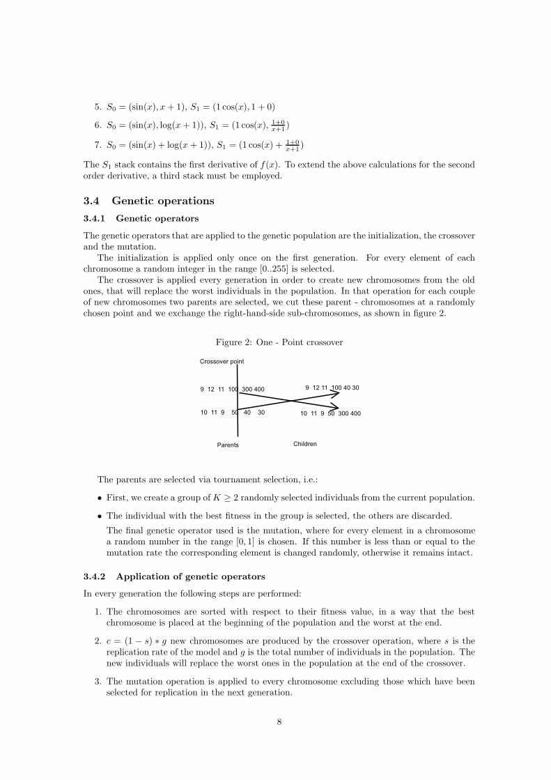
The crossover is applied every generation in order to create new chromosomes from the oldones, that will replace the worst individuals in the population. In that operation for each coupleof new chromosomes two parents are selected, we cut these parent - chromosomes at a randomlychosen point and we exchange the right-hand-side sub-chromosomes, as shown in figure 2.
Figure 2: One - Point crossover
The parents are selected via tournament selection, i.e.:
• First, we create a group of K ≥ 2 randomly selected individuals from the current population.
• The individual with the best fitness in the group is selected, the others are discarded.
The final genetic operator used is the mutation, where for every element in a chromosomea random number in the range [0, 1] is chosen. If this number is less than or equal to themutation rate the corresponding element is changed randomly, otherwise it remains intact.
3.4.2 Application of genetic operators
In every generation the following steps are performed:
1. The chromosomes are sorted with respect to their fitness value, in a way that the bestchromosome is placed at the beginning of the population and the worst at the end.
2. c = (1 − s) ∗ g new chromosomes are produced by the crossover operation, where s is thereplication rate of the model and g is the total number of individuals in the population. Thenew individuals will replace the worst ones in the population at the end of the crossover.
3. The mutation operation is applied to every chromosome excluding those which have beenselected for replication in the next generation.
8
3.5 Termination control
The genetic operators are applied to the population creating new generations, until a maximumnumber of generations is reached or the best chromosome in the population has fitness better thana preset threshold.
4 Experimental results
We describe several experiments performed on linear and non linear first and second order ODE’sand systems and PDE’s in two and three dimensions. In addition we applied our method to ODE’sthat do not posses an analytical closed form solution and hence can not be represented exactly bythe grammar. For the case of systems of ODE’s, each chromosome is split uniformly in M parts,where M is the number of equations in the system. Each part of the chromosome represents thesolution of the corresponding ODE. We used 10% for the replication rate (hence the crossoverprobability is set to 90%) and 5% for the mutation rate. We investigated the importance of thesetwo parameters by performing experiments using sets of different values. Each experiment wasperformed 30 times and we plot the average number of generations for the ODE7 problem in figure3. As one can see the performance is somewhat dependent on these parameters, but not critically.The population size was set to 1000 and the length of each chromosome to 50. The size of thepopulation is a critical parameter. Too small a size weakens the method’s effectiveness. Too biga size renders the method slow. Hence since there is no first principals estimation for the thepopulation size, we resorded to an experimental approach to obtain a realistic determination ofits range. It turns out that values in the interval [200, 1000] are proper. We used fixed - lengthchromosomes instead of variable - length to avoid creation of unnecessary large chromosomeswhich will render the method inefficient. The length of the chromosomes is usually depended onthe problem to be solved. For the case of simple ODE’s a length between 20 and 50 is usuallysufficient, while for the case of SODE’s and PDE’s where the chromosome must be split into parts,the length must be increased accordingly. The experiments were performed on an AMD ATHLON2400+ running Slackware Linux 9.1 The penalty parameter λ in the penalty function was setto 100 in all runs, except for PDE cases where the value λ = 1 was sufficient. The maximumnumber of generations allowed was set to 2000 and the preset fitness target for the terminationcriteria was 10−7. From the conducted experiments, we have observed that the maximum numberof generations allowed must be greater for difficult problems such as SODE’s and PDE’s than forsimpler problems of ODE’s. The value of N for ODE’s was between 10 and 20 depending on theproblem. For PDE’s N was set to 5 (i.e. 52 = 25 points) and Nx = Ny = 50. We tried to selectthe value for N and Nx so as to minimize the computational effort without sacrificing quality.The results were compared against the results from the DSolve procedure of the Mathematicaprogram version 5.0 running on Mandrake Linux v10.0. According to the manual of Mathematicathe DSolve procedure can solve linear ordinary differential equations with constant coefficients.Also, it can solve many linear equations up to second order with non - constant coefficients and itincludes general procedures that handle a large fraction of the nonlinear ODE’s whose solutionsare given in standard reference books such as Kamke [22]. The evaluation of the derived functionswas performed using the FunctionParser programming library [3].
9
Figure 3: Average number of generations versus the replication rate for two values of the mutationrate ( problem ODE7)
250
300
350
400
450
500
550
600
650
700
0.05 0.1 0.15 0.2 0.25 0.3 0.35 0.4 0.45
gene
ratio
ns(a
vera
ge)
replication rate
mutation: 5%mutation: 10%
4.1 Linear ODE’s
In the present subsection we present the results from first and second order linear ODE’s. Theproposed was applied in each equation 30 times and in every experiment the analytical solutionwas found.
ODE1
y′ =2x − y
x
with y(0) = 20.1 and x ∈ [0.1, 1.0]. The analytical solution is y(x) = x + 2x.
ODE2
y′ =1 − y cos(x)
sin(x)
with y(0.1) = 2.1sin(0.1) and x ∈ [0.1, 1]. The analytical solution is y(x) = x+2
sin(x) .
ODE3
y′ = −1
5y + exp(−x
5) cos(x)
with y(0) = 0 and x ∈ [0, 1]. The analytical solution is y(x) = exp(− x5 ) sin(x).
ODE4
y′′ = −100y
with y(0) = 0 and y′(0) = 10 and x ∈ [0, 1]. The analytical solution is y(x) = sin(10x).
10
ODE5
y′′ = 6y′ − 9y
with y(0) = 0 and y′(0) = 2 and x ∈ [0, 1]. The analytical solution is y(x) = 2x exp(3x).
ODE6
y′′ = −1
5y′ − y − 1
5exp(−x
5) cos(x)
with y(0) = 0 and y′(0) = 1 and x ∈ [0, 2]. The analytical solution is y(x) = exp(− x5 ) sin(x).
ODE7
y′′ = −100y
with y(0) = 0 and y(1) = sin(10) and x ∈ [0, 1]. The analytical solution is y(x) = sin(10x).
ODE8
xy′′ + (1 − x)y′ + y = 0
with y(0) = 1 and y(1) = 0 and x ∈ [0, 1]. The analytical solution is y(x) = 1 − x.
ODE9
y′′ = −1
5y′ − y − 1
5exp(−x
5) cos(x)
with y(0) = 0 and y(1) = sin(1)exp(0.2) and x ∈ [0, 1]. The analytical solution is y(x) = exp(− x
5 ) sin(x).
In table 2 we list the results from the proposed method for the equations above. Under the ODEheading the equation label is listed. Under the headings MIN, MAX, AVG we list the minimum,maximum and average number of generations (in the set of 30 experiments) needed to recover theexact solution. The Mathematica subroutine DSolve has managed to find the analytical solutionin all cases.
In figure 4 we plot the evolution of a trial solution for the fourth problem of table 2. Atgeneration 22 the fitness value was 4200.5 and the intermediate solution was:
Finally, at generation 59 the problem was solved exactly.
Figure 4: Evolving candidate solutions of y′ = −100y with boundary conditions on the left
-1
-0.8
-0.6
-0.4
-0.2
0
0.2
0.4
0.6
0.8
1
0 0.2 0.4 0.6 0.8 1
y22(x)y27(x)
y(x)
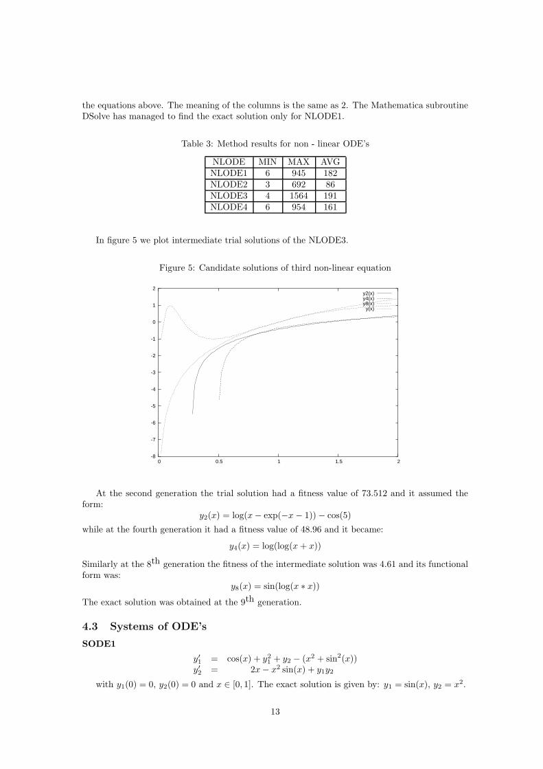
4.2 Non - linear ordinary differential equations
In this subsection we present results from the application of the method to non - linear ordi-nary differential equations. In all the equations the method was applied 30 times and in everyapplication the exact solution was found.
NLODE1
y′ =1
2y
with y(1) = 1 and x ∈ [1, 4]. The exact solution is y =√
with y(1) = 1 + sin(1) and x ∈ [1, 2] The exact solution is y = x + sin(x).
NLODE3
y′′y′ = − 4
x3
with y(1) = 0 and x ∈ [1, 2]. The exact solution is y = log(x2).
NLODE4
x2y′′ + (xy′)2 +1
log(x)= 0
with y(e) = 0, y′(e) = 1e
and x ∈ [e, 2e]. The exact solution is y(x) = log(log(x)) and it was
recovered at the 30th generation. In table 3 we list results from the application of the method to
12
the equations above. The meaning of the columns is the same as 2. The Mathematica subroutineDSolve has managed to find the exact solution only for NLODE1.
Table 3: Method results for non - linear ODE’s
NLODE MIN MAX AVGNLODE1 6 945 182NLODE2 3 692 86NLODE3 4 1564 191NLODE4 6 954 161
In figure 5 we plot intermediate trial solutions of the NLODE3.
Figure 5: Candidate solutions of third non-linear equation
-8
-7
-6
-5
-4
-3
-2
-1
0
1
2
0 0.5 1 1.5 2
y2(x)y4(x)y8(x)y(x)
At the second generation the trial solution had a fitness value of 73.512 and it assumed theform:
y2(x) = log(x − exp(−x − 1)) − cos(5)
while at the fourth generation it had a fitness value of 48.96 and it became:
y4(x) = log(log(x + x))
Similarly at the 8th generation the fitness of the intermediate solution was 4.61 and its functionalform was:
y8(x) = sin(log(x ∗ x))
The exact solution was obtained at the 9th generation.
with y1(0) = 0, y2(0) = 0 and x ∈ [0, 1]. The exact solution is given by: y1 = sin(x), y2 = x2.
13
SODE2
y′1 = cos(x)−sin(x)
y2
y′2 = y1y2 + exp(x) − sin(x)
with y1(0) = 0, y2(0) = 1 and x ∈ [0, 1]. The exact solution is y1 = sin(x)exp(x) , y2 = exp(x).
SODE3
y′1 = cos(x)
y′2 = −y1
y′3 = y2
y′4 = −y3
y′5 = y4
with y1(0) = 0, y2(0) = 1, y3(0) = 0,y4(0) = 1, y5(0) = 0 and x ∈ [0, 1]. The exact solutions isy1 = sin(x), y2 = cos(x), y3 = sin(x), y4 = cos(x), y5 = sin(x).
SODE4
y′1 = − 1
y2
sin(exp(x))
y′2 = −y2
with y1(0) = cos(1.0), y2(0) = 1.0 and x ∈ [0, 1]. The exact solution is y1 = cos(exp(x)),y2 = exp(−x). In table 4 we list results from the application of the method to the equationsabove. The meaning of the columns is the same as 2. The Mathematica subroutine DSolve hasmanaged to find the analytical solution only for SODE3.
Table 4: Method results for non - linear ODE’s
SODE MIN MAX AVGSODE1 6 1211 201SODE2 15 1108 234SODE3 30 1205 244SODE4 5 630 75
4.4 An ODE without an analytical closed form solution
Example 1
y′′ +1
xy′ − 1
xcos(x) = 0
with x ∈ [0, 1] and y(0) = 0 and y′(0) = 1. With 20 points in [0,1] we find:
GP1(x) = x(cos(− sin(x/3 + exp(−5 + x − exp(cos(x)))))))
with fitness value 2.1 ∗ 10−6. The exact solution is :
y(x) =
∫ x
0
sin(t)
tdt
In figure 6, we plot the two functions in the range [0,5]
14
Figure 6: Plot of GP1(x) and y(x) =∫ x
0sin(t)
tdt
0
0.5
1
1.5
2
2.5
3
0 0.5 1 1.5 2 2.5 3 3.5 4 4.5 5
GP1(x)y(x)
Example 2
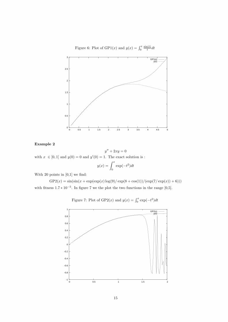
y′′ + 2xy = 0
with x ∈ [0, 1] and y(0) = 0 and y′(0) = 1. The exact solution is :
with fitness 1.7 ∗ 10−5. In figure 7 we the plot the two functions in the range [0,5].
Figure 7: Plot of GP2(x) and y(x) =∫ x
0 exp(−t2)dt
-1
-0.8
-0.6
-0.4
-0.2
0
0.2
0.4
0.6
0.8
1
0 0.5 1 1.5 2
GP2(x)y(x)
15
Observe, that even though the equations in the above examples were solved for x ∈ [0, 1],the approximation maintains its quality beyond that interval, a fact that illustrates the unusualgeneralization ability.
4.5 A special case
Consider the ODEy′′(x2 + 1) − 2xy − x2 − 1 = 0
in the range [0, 1] and with initial conditions y(0) = 0 and y′(0) = 1. The analytical solution isy(x) = (x2 + 1)arctan(x). Note that arctan(x) does not belong to the function repertoire of themethod and this make the case special. The solution reached is not exact but approximate givenby:
with fitness 0.0059168. Note that the subroutine DSolve of Mathematica failed to solve theabove equation. In figure 8 we plot z(x) ( obtained using the method of Lagaris et al [5]),y(x) = (x2 +1)arctan(x) (which is the exact solution) and the above solution GP(x). From figures6, 7 and 8 we observe the quality of the approximate solution even outside the training interval,hence rendering our method useful and practical.
Figure 8: z(x), y(x) = (x2 + 1)arctan(x), GP(x)
0
1
2
3
4
5
6
7
0 0.5 1 1.5 2
z(x)y(x)
GP(x)
4.6 PDE’s
In this subsection we present results from the application of the method to elliptic partial differ-ential equations. In all the equations the method was applied 30 times and in every applicationthe exact solution was found.
16
PDE1
∇2Ψ(x, y) = exp(−x)(x − 2 + y3 + 6y)
with x ∈ [0, 1] and y ∈ [0, 1] and boundary conditions:Ψ(0, y) = y3, Ψ(1, y) = (1 + y3) exp(−1),Ψ(x, 0) = x exp(−x), Ψ(x, 1) = (x+1) exp(−x). The exact solution is Ψ(x, y) = (x+y3) exp(−x).
PDE2
∇2Ψ(x, y) = −2Ψ(x, y)
with x ∈ [0, 1] and y ∈ [0, 1] and boundary conditions: Ψ(0, y) = 0, Ψ(1, y) = sin(1) cos(y),Ψ(x, 0) = sin(x), Ψ(x, 1) = sin(x) cos(1). The exact solution is Ψ(x, y) = sin(x) cos(y).
PDE3
∇2Ψ(x, y) = 4
with x ∈ [0, 1] and y ∈ [0, 1] and boundary conditions:Ψ(0, y) = y2 + y + 1, Ψ(1, y) = y2 + y + 3,Ψ(x, 0) = x2 + x + 1, Ψ(x, 1) = x2 + x + 3. The exact solution is Ψ(x, y) = x2 + y2 + x + y + 1.
PDE4
∇2Ψ(x, y) = −(x2 + y2)Ψ(x, y)
with x ∈ [0, 1] and y ∈ [0, 1] and boundary conditions:Ψ(x, 0) = 0, Ψ(x, 1) = sin(x), Ψ(0, y) = 0,Ψ(1, y) = sin(y). The exact solution is Ψ(x, y) = sin(xy).
PDE5
∇2Ψ(x, y) = (x − 2) exp(−x) + x exp(−y)
with x ∈ [0, 1] and y ∈ [0, 1] and boundary conditions: Ψ(x, 0) = x(exp(−x) + 1), Ψ(x, 1) =x(exp(−x)+exp(−1)), Ψ(0, y) = 0, Ψ(1, y) = exp(−y)+exp(−1). The exact solution is Ψ(x, y) =x(exp(−x) + exp(−y)).
PDE6
The following is a highly non - linear pde:
∇2Ψ(x, y) + exp(Ψ(x, y)) = 1 + x2 + y2 +4
(1 + x2 + y2)2
with x ∈ [−1, 1] and y ∈ [−1, 1] and boundary conditions: f(0, y) = log(1+y2), f(1, y) = log(2+y2), g(x, 0) = log(1+x2) and g(x, 1) = log(2+x2). The exact solution is Ψ(x, y) = log(1+x2+y2).
PDE7
∇2Ψ(x, y, z) = 6
with x ∈ [0, 1] and y ∈ [0, 1] and z ∈ [0, 1] and boundary conditions: Ψ(0, y, z) = y2 + z2,Ψ(1, y, z) = y2 + z2 + 1, Ψ(x, 0, z) = x2 + z2, Ψ(x, 1, z) = x2 + z2 + 1, Ψ(x, y, 0) = x2 + y2,Ψ(x, y, 1) = x2 + y2 + 1. The exact solution is Ψ(x, y, z) = x2 + y2 + z2 + 1.
In table 5 we list results from the application of the method to the equations above. Themeaning of the columns is the same as 2. The Mathematica subroutine DSolve has not managedto find the exact solution for any of the examples above.
In the following we present some graphs for trial solutions of the second PDE. At generation1 the trial solution was
GP1(x, y) =x
7
with fitness value 8.14. The difference between the trial solution GP1(x, y) and the exact solution
Ψ(x, y) is shown in figure 9. At the 10thgeneration the trial solution was
GP10(x, y) = sin(x/3 + x)
with fitness value 3.56. The difference between the trial solution GP10(x, y) and the exact solutionΨ(x, y) is shown in figure 10.
Figure 9: Difference between Ψ(x, y) = sin(x) cos(y) and GP1(x, y)
0 0.2
0.4 0.6
0.8 1 0
0.2
0.4
0.6
0.8
1
0
0.1
0.2
0.3
0.4
0.5
0.6
0.7
18
Figure 10: Difference between Ψ(x, y) = sin(x) cos(y) and GP10(x, y)
0 0.2
0.4 0.6
0.8 1 0
0.2
0.4
0.6
0.8
1
-0.6
-0.5
-0.4
-0.3
-0.2
-0.1
0
At the 40th generation the trial solution was
GP40(x) = sin(cos(y)x)
with fitness value 0.59. The difference between the trial solution GP40(x, y) and the exact solutionΨ(x, y) is shown in figure 11.
Figure 11: Difference between Ψ(x, y) = sin(x) cos(y) and GP40(x, y)
0 0.2
0.4 0.6
0.8 1 0
0.2
0.4
0.6
0.8
1
-0.06
-0.05
-0.04
-0.03
-0.02
-0.01
0
5 Conclusions and further work
We presented a novel approach for solving ODE’s and PDE’s. The method is based on geneticprogramming. This approach creates trial solutions and seeks to minimize an associated error.
19
The advantage is that our method can produce trial solutions of highly versatile functional form.Hence the trial solutions are not restricted to a rather inflexible form that is imposed frequently bybasis - set methods that rely on completeness. If the grammar has a rich function repertoire, andthe differential equation has a closed form solution, it is very likely that our method will recoverit. If however the exact solution can not be represented in a closed form, our method will producea closed form approximant.
The grammar used in this article can be further developed and enhanced. For instance itis straight forward to enrich the function repertoire or even to allow for additional operations.Treating different types of PDE’s with the appropriate boundary conditions is a topic of currentinterest and is being investigated. Our preliminary results are very encouraging.
References
1. J.D. Lambert, Numerical methods for Ordinary Differential Systems: The initial value prob-lem, John Wiley & Sons: Chichester, England, 1991.
2. J. R. Koza, Genetic Programming: On the programming of Computer by Means of NaturalSelection. MIT Press: Cambridge, MA, 1992.
3. J. Nieminen and J. Yliluoma, “Function Parser for C++, v2.7”, available fromhttp://www.students.tut.fi/̃ warp/FunctionParser/.
4. G. E. Fasshauer, “Solving Differential Equations with Radial Basis Functions: MultilevelMethods and Smoothing,” Advances in Computational Mathematics, vol. 11, No. 2-3, pp.139-159, 1999.
5. I. Lagaris, A. Likas, and D.I. Fotiadis, “Artificial Neural Networks for Solving Ordinary andPartial Differential Equations,” IEEE Transactions on Neural Networks, vol. 9, No. 5, pp.987-1000, 1998.
6. G. Burgess, “Finding Approximate Analytic Solutions to Differential Equations Using Ge-netic Programming,” Surveillance Systems Division, Electronics and Surveillance ResearchLaboratory, Department of Defense, Australia, 1999.
7. Cao, H., Kang, L., Chen, Y., Yu, J., Evolutionary Modeling of Systems of Ordinary DifferentialEquations with Genetic Programming, Genetic Programming and Evolvable Machines, vol.1,pp.309-337, 2000.
8. Iba,H., Sakamoto,E.: ”Inference of Differential Equation Models by Genetic Programming”,Proceedings of the Genetic and Evolutionary Computation Conference (GECCO 2002),pp.788-795, 2002.
9. M. O’ Neill, Automatic Programming in an Arbitrary Language: Evolving Programs withGrammatical Evolution. PhD thesis, University Of Limerick, Ireland, August 2001.
10. C. Ryan, J. J. Collins and M. O’ Neill, Evolving programs for an arbitrary language.In Wolf-gang Banzhaf, Riccardo Poli, Marc Schoenauer, and Terence C. Fogarty, editors, Proceedingsof the First European Workshop on Genetic Programming, volume 1391 of LNCS, pages 83–95,Paris, 14-15 April 1998. Springer-Verlag.
11. M. O’Neill and C. Ryan, Grammatical Evolution: Evolutionary Automatic Programming in aArbitrary Language, volume 4 of Genetic programming. Kluwer Academic Publishers, 2003.
12. C. Ryan, M. O’Neill, and J.J. Collins, “Grammatical Evolution: Solving Trigonometric Iden-tities,” In proceedings of Mendel 1998: 4th International Mendel Conference on Genetic Al-gorithms, Optimization Problems, Fuzzy Logic, Neural Networks, Rough Sets., Brno, CzechRepublic, June 24-26 1998. Technical University of Brno, Faculty of Mechanical Engineering,pp. 111-119.
20
13. M. O’Neill and C. Ryan, “Grammatical Evolution,” IEEE Trans. Evolutionary Computation,Vol. 5, pp. 349-358, 2001.
14. D.E. Goldberg, Genetic algorithms in search, Optimization and Machine Learning, AddisonWesley, 1989.
15. J.J Collins and C. Ryan, “Automatic Generation of Robot Behaviors using GrammaticalEvolution,” In Proc. of AROB 2000, the Fifth International Symposium on Artificial Life andRobotics.
16. M. O’Neill, J.J. Collins and C. Ryan, “Automatic generation of caching algorithms,” In KaisaMiettinen, Marko M. Mkel, Pekka Neittaanmki, and Jacques Periaux (eds.), EvolutionaryAlgorithms in Engineering and Computer Science, Jyvskyl, Finland, 30 May - 3 June 1999,John Wiley & Sons, pp. 127-134, 1999.
17. A. Brabazon and M. O’Neill, “A grammar model for foreign-exchange trading,” In H. R.Arabnia et al., editor, Proceedings of the International conference on Artificial Intelligence,volume II, CSREA Press, 23-26 June 2003, pp. 492-498, 2003.
18. P. Cusdin and J.D. Muller, “Automatic Differentiation and Sensitivity Analysis Methods forCFD,” QUB School of Aeronautical Engineering, 2003.
19. O. Stauning, ”Flexible Automatic Differentiation using Templates and Operator Overloadingin C++,” Talk presented at the Automatic Differentiation Workshop at Shrivenham Campus,Cranfield University, June 6, 2003.
20. C. Bischof, A. Carle, G. Corliss, and A. Griewank, “ADIFOR - Generating Derivative Codesfrom Fortran Programs,” Scientific Programming, no. 1, pp. 1-29, 1992.
21. A. Griewank, ”On Automatic Differentiation” in M. Iri and K. Tanabe (eds.), MathematicalProgramming: Recent Developments and Applications, Kluwer Academic Publishers, Ams-terdam, pp. 83-108, 1989.
22. E. Kamke: Differential Equations. Solution Methods and Solutions, Teubner, Stuttgart, 1983.


![[George v. Tsoulos] Adaptive Antennas for Wireless(BookZZ.org)](https://static.documents.pub/doc/80x56/5695d0d11a28ab9b0293fd44/george-v-tsoulos-adaptive-antennas-for-wirelessbookzzorg.jpg)


