30
Solving Nonlinear Equations Jijian Fan Department of Economics University of California, Santa Cruz Oct 13 2014

Solving Nonlinear Equations
Jijian Fan
Department of EconomicsUniversity of California, Santa Cruz
Oct 13 2014

Overview
NUMERICALLY solving nonlinear equation
f(x) = 0
Four methodsBisectionFunction iterationNewton’sQuasi-Newton

Motivation
Linear equation can be solved analyticallyAx = b ⇒ x = A−1bMethods such as L-U factorization, Gaussian elimination,etc
However, nonlinear equation might not be explicitly solvede.g. f(x) = x−0.8 + 2x0.5 − 3 = 0Numerical methods

Motivation
Linear equation can be solved analyticallyAx = b ⇒ x = A−1bMethods such as L-U factorization, Gaussian elimination,etc
However, nonlinear equation might not be explicitly solvede.g. f(x) = x−0.8 + 2x0.5 − 3 = 0Numerical methods

Numerical methods
"Continuous" means 1, 1.001, . . . , 1.999, 2"Equality" means 1 = 1.0003
Figure 1 : A "continuous" function in computer

Bisection Method
Based on Intermediate Value TheoremStart with a bounded interval [a, b] such that f(a)f(b) < 0
Sample codewhile (b-a)>tol;
if sign(f((a+b)/2)) == sign(f(a))a= (a+b)/2;
elseb= (a+b)/2;
endx=a;

Bisection Method
AdvantageReliable: always finds the rootLEAST requirements on functional properties
DisadvantageUnivariate f : R 7→ RSlow log(n)

Function Iteration
Solve for fixed point x = g(x)f(x) = 0⇔ x = g(x) = x− f(x)
Start with an initial guess x(0) s.t. ||g′(x(0))|| < 1
Sample codex=x0;y=g(x);while norm(y-x)>tol;
x=y;y=g(x);
end

Function Iteration
AdvantageCould be multivariate f : Rn 7→ Rn
Easy-coding
DisadvantageNot reliable: require differentiability, andInitial x(0) should be sufficiently close to a fixed point x∗Only applicable to downward-crossing fixed point||g′(x∗)|| < 1Worth trying even if one or more condition fails

Function Iteration: Extension
Value Function Iteration (VFI)
V(k) = maxk′{u(c) + βV(k′)}
k′ = f(k)− c+ (1− δ)k
Rewrite as
V(k) = maxk′{u(f(k) + (1− δ)k− k′) + βV(k′)}
Function Iteration: Extension
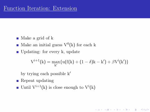
Make a grid of kMake an initial guess V0(k) for each kUpdating: for every k, update
Vi+1(k) = maxk′{u(f(k) + (1− δ)k− k′) + βVi(k′)}
by trying each possible k′
Repeat updatingUntil Vi+1(k) is close enough to Vi(k)

Newton’s Method
First-order Taylor approximation
f(x) ≈ f(x(k)) + f ′(x(k))(x− x(k)) = 0
Solve for the iteration rule
x(k+1) ← x(k) − [f ′(x(k))]−1f(x(k))
Start with an initial guess x(0)
Pseudo-codefor iter=1:maxiter
[ fval fjac ]=f(x);x = x - fjac \ fval;if norm(fval) < tol, break, end
end

Newton’s Method
First-order Taylor approximation
f(x) ≈ f(x(k)) + f ′(x(k))(x− x(k)) = 0
Solve for the iteration rule
x(k+1) ← x(k) − [f ′(x(k))]−1f(x(k))
Start with an initial guess x(0)
Pseudo-codefor iter=1:maxiter
[ fval fjac ]=f(x);x = x - fjac \ fval;if norm(fval) < tol, break, end
end

Newton’s Method: Calculate the Jacobian Matrix
How to calculate the Jacobian Matrix
f ′(x) =
∂f1/∂x1 ∂f1/∂x2 . . . ∂f1/∂xn∂f2/∂x1 ∂f2/∂x2 . . . ∂f2/∂xn
......
. . ....
∂fn/∂x1 ∂fn/∂x2 . . . ∂fn/∂xn
Analytical derivativesNumerical derivatives

Newton’s Method: Calculate the Jacobian Matrix
Analytical derivatives example: Cournot duopoly model
P(q) = q−1/η
Ci(qi) =12ciq2
i
maxqi
πi(q1, q2) = P(q1 + q2)qi − Ci(qi)
F.O.C.∂πi
∂qi= P(q1 + q2) + P′(q1 + q2)qi − C′i(qi) = 0
Let
~f(~q) =
[∂π1∂q1
(q1, q2)∂π2∂q2
(q1, q2)
]Solve
~f(~q) = ~0

Newton’s Method: Calculate the Jacobian Matrix
Note that∂fi∂xj≡ ∂2πi
∂qj∂qi
function [fval,fjac]=f(q)c=[0.6,0.8]; eta=1.6; e=-1/eta;fval=sum(q)ˆe + e*sum(q)ˆ(e-1)*q-diag(c)*q;fjac=e*sum(q)ˆ(e-1)*ones(2,2)+e*sum(q)ˆ(e-1)*eye(2)+ (e-1)*e*sum(q)ˆ(e-2)*q*[1 1]-diag(c);
end

Newton’s Method: Calculate the Jacobian Matrix
Note that∂fi∂xj≡ ∂2πi
∂qj∂qi
function [fval,fjac]=f(q)c=[0.6,0.8]; eta=1.6; e=-1/eta;fval=sum(q)ˆe + e*sum(q)ˆ(e-1)*q-diag(c)*q;fjac=e*sum(q)ˆ(e-1)*ones(2,2)+e*sum(q)ˆ(e-1)*eye(2)+ (e-1)*e*sum(q)ˆ(e-2)*q*[1 1]-diag(c);
end
Newton’s Method: Calculate the Jacobian Matrix
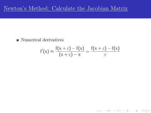
Numerical derivatives
f ′(x) ≈ f(x+ ε)− f(x)(x+ ε)− x
=f(x+ ε)− f(x)
ε
Centered finite difference approximation
f ′(x) ≈ f(x+ ε)− f(x− ε)(x+ ε)− (x− ε)
=f(x+ ε)− f(x− ε)
2ε

Newton’s Method: Calculate the Jacobian Matrix
Numerical derivatives
f ′(x) ≈ f(x+ ε)− f(x)(x+ ε)− x
=f(x+ ε)− f(x)
ε
Centered finite difference approximation
f ′(x) ≈ f(x+ ε)− f(x− ε)(x+ ε)− (x− ε)
=f(x+ ε)− f(x− ε)
2ε

Newton’s Method: Calculate the Jacobian Matrix
For multivariate case, let
ε =
0...0ε0...0

Quasi-Newton Methods
Calculating f ′(x) and taking inverse isSlowInefficient
GoalFind a proper approximation of f ′(x) or (f ′(x))−1
Update this approximation in a more efficient wayMethods
Secant methodBroyden’s method

Secant Methods
UnivariateApproximate derivatives (tangent) by secant
f ′(x(k)) ≈ f(x(k))− f(x(k−1))
x(k) − x(k−1)
thus
[f ′(x(k))]−1 ≈ x(k) − x(k−1)
f(x(k))− f(x(k−1))
Iteration rule
x(k+1) ← x(k) − x(k) − x(k−1)
f(x(k))− f(x(k−1))f(x(k))
Need two initial value

Secant Methods
UnivariateApproximate derivatives (tangent) by secant
f ′(x(k)) ≈ f(x(k))− f(x(k−1))
x(k) − x(k−1)
thus
[f ′(x(k))]−1 ≈ x(k) − x(k−1)
f(x(k))− f(x(k−1))
Iteration rule
x(k+1) ← x(k) − x(k) − x(k−1)
f(x(k))− f(x(k−1))f(x(k))
Need two initial value

Broyden’s Methods
Generalized secant method for multivariateDenote A(k) as the Jacobian approximant of f at x = x(k)
Newton iteration
x(k+1) ← x(k) − (A(k))−1f(x(k))
Secant condition must hold at x(k+1)
f(x(k+1))− f(x(k)) = A(k+1)(x(k+1) − x(k))
Broyden’s Methods
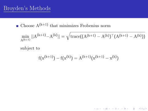
Choose A(k+1) that minimizes Frobenius norm
minA(k+1)
||A(k+1)−A(k)|| =√
trace((A(k+1) −A(k))>(A(k+1) −A(k)))
subject to
f(x(k+1))− f(x(k)) = A(k+1)(x(k+1) − x(k))
Solve for A(k+1)
A(k+1) ← A(k) + [f(x(k+1))− f(x(k))−A(k)d(k)]d(k)>
d(k)>d(k)
whered(k) = x(k+1) − x(k)

Broyden’s Methods
Choose A(k+1) that minimizes Frobenius norm
minA(k+1)
||A(k+1)−A(k)|| =√
trace((A(k+1) −A(k))>(A(k+1) −A(k)))
subject to
f(x(k+1))− f(x(k)) = A(k+1)(x(k+1) − x(k))
Solve for A(k+1)
A(k+1) ← A(k) + [f(x(k+1))− f(x(k))−A(k)d(k)]d(k)>
d(k)>d(k)
whered(k) = x(k+1) − x(k)
Broyden’s Methods
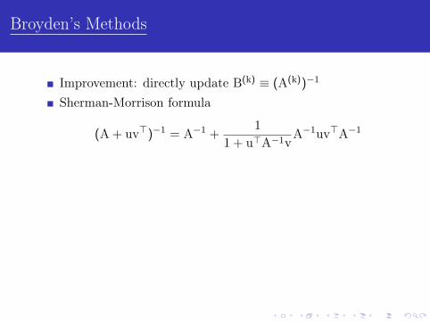
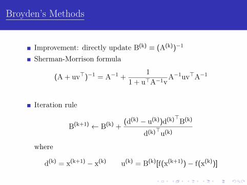
Improvement: directly update B(k) ≡ (A(k))−1
Sherman-Morrison formula
(A+ uv>)−1 = A−1 +1
1+ u>A−1vA−1uv>A−1
Iteration rule
B(k+1) ← B(k) +(d(k) − u(k))d(k)>B(k)
d(k)>u(k)
where
d(k) = x(k+1) − x(k) u(k) = B(k)[f(x(k+1))− f(x(k))]
Broyden’s Methods
Improvement: directly update B(k) ≡ (A(k))−1
Sherman-Morrison formula
(A+ uv>)−1 = A−1 +1
1+ u>A−1vA−1uv>A−1
Iteration rule
B(k+1) ← B(k) +(d(k) − u(k))d(k)>B(k)
d(k)>u(k)
where
d(k) = x(k+1) − x(k) u(k) = B(k)[f(x(k+1))− f(x(k))]

Broyden’s Methods
Pseudo-code
Choose initial xCalculate initial B (usually B = f ′−1(x))loop
update xif f(x) is close enough to 0 then breakupdate B
end
Summary
Four method to solve nonlinear equationsBisection: robust but relatively slowFunction iteration: easy-codingNewton & Quasi-Newton: quick, most popular but notalways work
May not work for the multi-root case


