28
Solving parabolic PDEs in half precision Matteo Croci & Mike Giles Mathematical Institute University of Oxford SIAM Conference on Computational Science and Engineering 2021

Solving parabolic PDEs in half precision
Matteo Croci & Mike GilesMathematical InstituteUniversity of Oxford
SIAM Conference on Computational Science and Engineering 2021

Objective: developing low-precision PDE solvers
M. Croci PDEs in half precision

Overview
Background
A 3-step guide to solving the heat equation in low precision
M. Croci PDEs in half precision

Round to nearest
xk x xk+1
ϑ(xk+1 − xk),
ϑ ∈ [0, 1].
if ϑ < 0.5
if ϑ > 0.5
fl(x) = x(1 + δ), with |δ| ≤ u.
M. Croci PDEs in half precision

Stochastic rounding
xk x xk+1
ϑ(xk+1 − xk),
ϑ ∈ [0, 1].
with probability 1− ϑwith probability ϑ
sr(x) = x(1 + δ(ω)), with |δ(ω)| ≤ 2u, and E[sr(x)] = x .
M. Croci PDEs in half precision

RtN might cause stagnation
xk+1xk xk + ∆x
M. Croci PDEs in half precision

RtN might cause stagnation
xk+1xk xk + ∆x
M. Croci PDEs in half precision

SR is resilient to stagnation
xk+1xk xk + ∆x
M. Croci PDEs in half precision
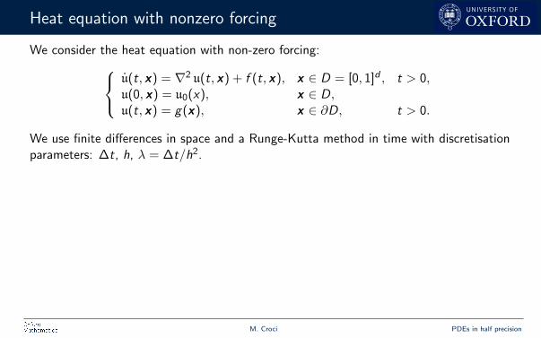
Heat equation with nonzero forcing
We consider the heat equation with non-zero forcing:
u(t, x) = ∇2 u(t, x) + f (t, x), x ∈ D = [0, 1]d , t > 0,u(0, x) = u0(x), x ∈ D,u(t, x) = g(x), x ∈ ∂D, t > 0.
We use finite differences in space and a Runge-Kutta method in time with discretisationparameters: ∆t, h, λ = ∆t/h2.
Let A be the (spd) stiffness matrix. The numerical scheme is:
Un+1 = SUn + ∆tF n
for some matrix S dependent on ∆tA. For instance,
Un+1 = (I −∆tA)Un + ∆tF nFE, (FE), Un+1 = (I + ∆tA)−1Un + ∆tF n
BE, (BE).
We work in bfloat16 half precision, u = 2−8 ≈ 4× 10⁻³.Everything extends to FEM and linear parabolic equations.
M. Croci PDEs in half precision

Overview
Background
A 3-step guide to solving the heat equation in low precision
M. Croci PDEs in half precision

1) Local rounding errors and the delta form
How to best implement the Runge-Kutta scheme? Use the delta form!
Standard form: Un+1 = SUn + ∆tF n.
Delta form: Un+1 = Un + ∆t(−SAUn + F n
)= Un + ∆Un.
e.g. SFE = (I −∆tA), SFE = 1, and SBE = SBE = (I + ∆tA)−1.
• Errors in the computation of SUn are of order u (machine precision).
• Errors in the computation of ∆Un are of order ∆tpu, p ≥ 0.
We prove that:
• The delta form produces much smaller rounding errors at each time step.
• Most of the rounding errors in the delta form are introduced into the final addition.
M. Croci PDEs in half precision

2) Exploit exact subtraction
How to best implement the matrix-vector product −AUn?
Uni+1 − 2Un
i + Uni−1
h2,
(Uni+1 −Un
i )− (Uni −Un
i−1)
h2.
Leads to O(h−2) error! Leads to near-exact matvecs.
A similar trick works for FEM as well. Only requires small modification of CSR matvecs.
Parts of a Theorem [C. and Giles 2020]
If a, b ∈ R are exactly represented in floating point arithmetic, and
|a− b| ≤ min(|a|, |b|)
then (a− b) is computed exactly.
See also Section 2.5 in “Accuracy and Stability of Numerical Algorithms” by Nick Higham.
M. Croci PDEs in half precision

Worst-case local rounding errors in 2D
10−3 10−2
∆t
10−3
10−2
10−1
100
u−1max
n(||errn|| ∞
/||U
N|| ∞
)RtN
FE
delta form
naive matvec
no delta form
O(∆t0.8)
BE
delta form
naive matvec
no delta form
O(∆t0.7)
BE
delta form
naive matvec
no delta form
O(∆t0.7)
10−4 10−3 10−2
∆t
10−3
10−2
10−1
100
u−1max
ω,n(||errn(ω)||
∞/||
UN(ω)||
∞)
SR
FE
delta form
naive matvec
no delta form
O(∆t1.1)
BE
delta form
naive matvec
no delta form
O(∆t0.7)
BE
delta form
naive matvec
no delta form
O(∆t0.7)
Note: from now on we use the delta form with “smart” matvecs.
M. Croci PDEs in half precision

3) RtN vs SR
Why is RtN in low precision bad for parabolic equations?
a) Stagnation:
• RtN always stagnates for sufficiently small ∆t (recall ∆Un = O(u∆tp)).
• The RtN solution is initial condition, discretization and precision dependent.
b) Global error:
• RtN rounding errors are strongly correlated and cannot be modelled as zero-meanindependent random variables.
• RtN global errors grow like O(u∆t−1) until stagnation.
SR fixes all these issues!
M. Croci PDEs in half precision

3a) Stagnation (left 1D, right 2D)
0.0 0.2 0.4 0.6 0.8 1.0x
0.4
0.6
0.8
1.0
1.2
1.4
1.6
1.8
2.0U
∞
double (same as exact)
SR, all initial conditions
RtN, u0 = 1
RtN, u0 = 3/2− |x− 1/2|RtN, u0 = 1 + noise
RtN, u0 = 1 + sin(8πx)
RtN computations are discretization and initial condition dependent. SR works!
M. Croci PDEs in half precision

3b) Global rounding errors [C. and Giles 2020]
Let εn ∈ RK be the vector containing all rounding errors introduced at time step n.
We can distinguish two cases:
RtN: we can only assume the worst-case scenario, |εni | ≤ ε = O(u) for all n, i .
SR: the εni are zero-mean spatially independent and temporally mean-independent.
Mode Norm 1D 2D 3D
RtN L2,∞ O(ε∆t−1) O(ε∆t−1) O(ε∆t−1)
SR E[|| · ||∞] O(ε∆t−1/4`(∆t)1/2) O(ε`(∆t)) O(ε`(∆t)1/2)
SR E[|| · ||2L2 ]1/2 O(ε∆t−1/4) O(ε`(∆t)1/2) O(ε)
Asymptotic global rounding error blow-up rates; `(∆t) = | log(λ−1∆t)|.Note that the RtN rates are well-known [Henrici 1962-1963, Jezequel 1995].
Spatial independence of SR errors means more error cancellation in higher dimensions!
M. Croci PDEs in half precision

3b) Global rounding errors (here at steady-state)
10−4 10−3 10−2
∆t
100
101
102
103
relative
error
∞ norm
RtN-FE
SR-FE
RtN-BE
SR-BE
O(∆t−1)
O(| log(∆t)|)
10−4 10−3 10−2
∆t
100
101
102
103
relative
error
L2 norm
RtN-FE
SR-FE
RtN-BE
SR-BE
O(∆t−1)
O(| log(∆t)|1/2)
Global error (delta form, 2D)
Note: relative error = error × (u||UN ||)−1
M. Croci PDEs in half precision

Outlook
• Working in low precision can bring large speed, memory and energy consumptionimprovements. New hardware supports low-precision.
• SR might be an effective way of obtaining accurate results in much lower precisionwhen solving time-dependent parabolic PDEs.
• Custom-built C++ low-precision emulator (bitbucket.org/croci/libchopping/)
inspired by [Higham and Pranesh 2019] and Milan Kloewer’s Julia routines(github.com/milankl?tab=repositories).
Current/future research directions
• Hyperbolic PDEs, stabilised explicit RK methods, nested multilevel Monte Carlo.
• Weather forecasting and brain simulation applications.
M. Croci PDEs in half precision

Thank you for listening!
Preprint, slides, and more info at: https://croci.github.io
[1] M. Croci and M. B. Giles. Effects of round-to-nearest and stochastic rounding in the numericalsolution of the heat equation in low precision, 2020. URL http://arxiv.org/abs/2010.16225.
[2] M. P. Connolly, N. J. Higham, and T. Mary. Stochastic Rounding and its Probabilistic BackwardError Analysis, 2020. URL https://hal.archives-ouvertes.fr/hal-02556997/document.
[3] N. J. Higham and T. Mary. A new approach to probabilistic rounding error analysis. SIAM Journalof Scientific Computing, 41(5):2815–2835, 2019. doi: 10.1137/18M1226312.
[4] N. J. Higham and S. Pranesh. Simulating low precision floating-point arithmetic. SIAM Journal onScientific Computing, 41(5):C585–C602, 2019. doi: 10.1137/19M1251308.
[5] N. J. Higham. Accuracy and Stability of Numerical Algorithms. SIAM, 2002.
[6] F. Jezequel. Round-off error propagation in the solution of the heat equation by finite differences.Journal of Universal Computer Science, 1(7):465–479, 1995.
[7] M. Arato. Round-off error propagation in the integration of ordinary differential equations by onestep methods. Acta Scientiarium Mathematicarum, 45:23–31, 1983. doi: 10.13140/2.1.3920.9608.
[8] P. Henrici. Discrete Variable Methods in Ordinary Differential Equations. John Wiley & Sons, Inc.,1962.
M. Croci PDEs in half precision

M. Croci PDEs in half precision
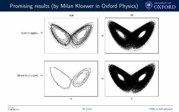
Promising results (by Milan Kloewer in Oxford Physics)
M. Croci PDEs in half precision
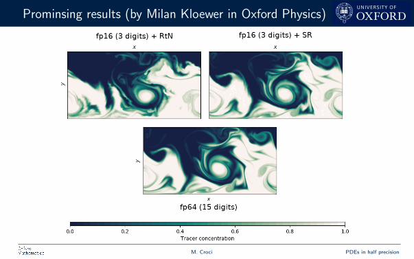
Prominsing results (by Milan Kloewer in Oxford Physics)
M. Croci PDEs in half precision

3a) Stagnation effects - theory
Stagnation fl(x + ε) = x occurs whenever u2 |x | ≥ |ε|. For the PDE:
u
2| u(tn, xi )| ≈
u
2|Un
i | ≥ |∆Uni | = |Un+1
i − Uni | ≈ ∆t|u(tn, xi )|,
This shows that Uni will not be updated whenever
| u(tn, xi )| ' 2(∆t/u)|u(tn, xi )|.
More formally,
Lemma [C. and Giles 2020]
Assume that the delta form is used and that p > 0. If there exists ε > 0 such that|U n
i | ≥ ε for some i , n, then there exists τ(ε) > 0 such that if ∆t < τ , we have
Uni = U n
i for all n ≥ n.
M. Croci PDEs in half precision


![Rigorous FEM for 1D Burgers equation[10,11,13,19,20,29] and parabolic [21,23–26,35] PDEs (but this mainly for periodic boundary conditions). The up to date information about these](https://static.documents.pub/doc/80x56/5ecc16849ccf4717d1558cd4/rigorous-fem-for-1d-burgers-equation-101113192029-and-parabolic-2123a2635.jpg)


![POST PROCESSING FOR STOCHASTIC PARABOLIC PARTIAL ...gabriel/Research/pp.pdf · Although inertial manifolds have been shown to exist for stochastic PDEs [2], we do not attempt to approximate](https://static.documents.pub/doc/80x56/5f3981f63b51e46d5c4709ac/post-processing-for-stochastic-parabolic-partial-gabrielresearchpppdf-although.jpg)
