Solving PDEs with PGI CUDA Fortran Part 4: Initial value...

Solving PDEs with PGI CUDA Fortran http://geo.mff.cuni.cz/~lh

Solving PDEs with PGI CUDA Fortran Part 4: Initial value problems for ordinary differential equations Outline ODEs and initial conditions. Explicit and implicit Euler methods. Runge-Kutta methods. Multistep Adams' predictor-corrector and Gear's BDF methods. Example: Lorenz attractor.


Ordinary differential equations and initial conditions 1 ordinary differential equation for 1 unknown function y(x) of 1 variable x For a unique solution, the initial condition is required A set of M ordinary differential equations for M unknown functions ym(x) of 1 variable x

for vector Y of unknown functions ym and vector F of right-hand-side functions fm For a unique solution, M initial conditions are required These are initial value problems (IVPs) for ordinary differential equations (ODEs). Higher-order ODEs can be rewritten into a set of 1st-order ODEs (see, e.g., Numerical Recipes).


Ordinary differential equations and initial conditions Discretization

x-grid and stepsize

numerical solution Numerical methods below are, for simplicity, formulated for 1 ODE and the constant stepsize h. However, they all also work for y replaced by Y and h replaced by hn.


Explicit Euler method the left-hand 1st-order finite-difference scheme for the 1st derivative after substitution into the ODE, we get the approximate explicit Euler method

it is an explicit formula as all terms on the right-hand side are known accuracy: 1st-order method (corresponds to the truncated Taylor expansion with the 0th and 1st term only)


Explicit Euler method stability: consider a linear problem with constant coefficients

(solution: ) Euler method: but for thus, there is a stepsize limit due to stability Pros: a simple explicit formula Cons: low accuracy => higher-order explicit methods low stability => implicit methods


Implicit Euler method the right-hand 1st-order finite-difference scheme for the 1st derivative after substitution into the ODE, we get the implicit Euler method

it is an implicit formula as there are references to unknown yn+1 on the right-hand side again, it is only 1-st order accurate


Implicit Euler method stability: as above, consider the problem (solution: ) the implicit formula: thus, implicit Euler method is stable for any (positive) h, it has an infinite region of absolute stability


Semi-implicit Euler method for solving implicit Euler method by linearization of F(Y) (similarly as in the Newton method for root finding)

i.e., in each step, MxM (Jacobian) matrix assembly and inversion is required


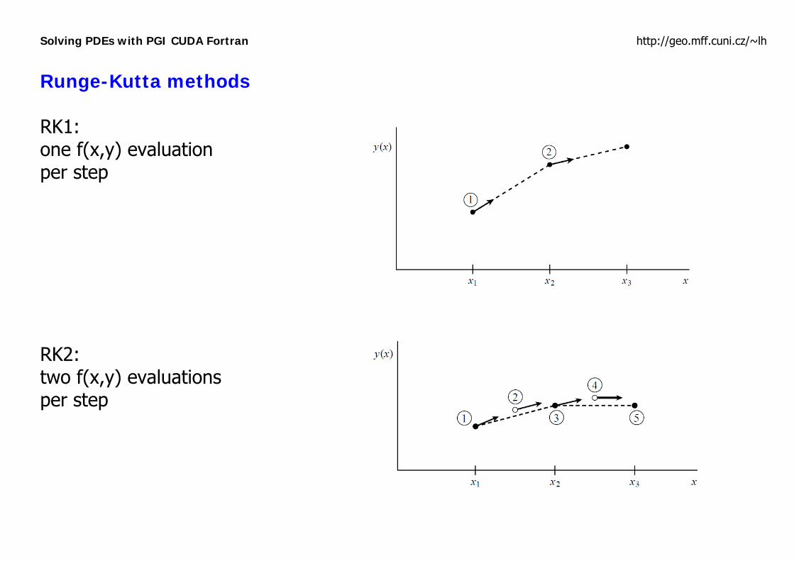
Runge-Kutta methods – more accurate, higher-order methods for integrating ODEs – approximate the Taylor expansion by averaging the appropriately chosen dy/dx along y(x) between xn and xn+1 – RK1: the explicit Euler method, the simplest RK method

for f(x) independent of y, it is equivalent to the rectangle quadrature rule – RK2: the 2nd-order RK method (midpoint method)

for f(x) independent of y, it is equivalent to the trapezoidal quadrature rule


Runge-Kutta methods RK1: one f(x,y) evaluation per step RK2: two f(x,y) evaluations per step


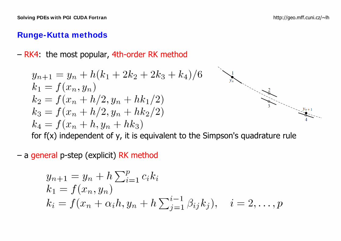
Runge-Kutta methods – RK4: the most popular, 4th-order RK method

for f(x) independent of y, it is equivalent to the Simpson's quadrature rule – a general p-step (explicit) RK method


Runge-Kutta methods – stepsize control (different h in each step): guess a step size, or make a few runs with step doubling, or use RK methods with adaptive stepsize control (e.g., Numerical Recipes, Chapter 16.2) – pros: higher accuracy, better stability (not as much as in implicit variants) than explicit Euler – implicit RK methods available (more stable than the explicit methods, but not infinitely stable)


Multistep methods A general linear multistep method

with or nonzero The methods are explicit and p-step for b0=0 and implicit and (p+1)-step otherwise.


Multistep methods Adams' family of multistep methods – based on polynomial approximation of f(x,y(x)) between xn+1-p and xn (xn+1 for implicit methods) and analytical integration of the approximating polynomial between xn and xn+1

– the order (i.e., the coincidence with the truncated Taylor expansion) is p for explicit and p+1 for implicit methods – the explicit p=1 method is the explicit Euler, the implicit p=0 method is the implicit Euler


Multistep methods Coefficients ai and bi of Adams' methods explicit (Adams-Bashforth) methods implicit (Adams-Moulton) methods all p: a1 = 1, other ai = 0 all p: a1 = 1, other ai = 0 i: 0 1 2 3 4 i: 0 1 2 3 4 p=0: bi – p=0: bi 1 p=1: bi 0 1 p=1: 2bi 1 1 p=2: 2bi 0 3 –1 p=2: 12bi 5 8 –1 p=3: 12bi 0 23 –16 5 p=3: 24bi 9 19 –5 1 p=4: 24bi 0 55 –59 37 –9 p=4: 720bi 251 646 –264 106 –19 e.g., explicit p=2: implicit p=1: Regions of absolute stability of explicit and implicit 2nd-order Adams methods


Multistep methods The predictor-corrector algorithm: conventional application of Adams' methods step P (predictor): applies an explicit Adams' formula of a given order, ynew = yn+1[explicit](xn+1) step E (evaluation): updates fn+1 = f(xn+1,ynew) step C (corrector): applies an implicit Adams' formula of the same order, ynew = yn+1[implicit](xn+1) steps E and C can be repeated: variants PEC, PECE, P(EC)2E i.e., a predictor extrapolates f into xn+1, a corrector makes use of this value for polynomial interpolation – initialization of multistep methods by their lower-order relatives or by RK methods – the predictor-corrector algorithm is essentially explicit, its stability is therefore worse than that of the corrector – adaptive stepsize control is laborious


Multistep methods Backward differentiation formulas (BDFs, Gear’s method) – based on polynomial approximation of y(x) between xn+1-p and xn+1 and analytical differentiation of the approximating polynomial at xn+1 – implicit p-step methods of the order p; for p=1: implicit Euler method – BDFs combined with the Newton method are known to have excellent stability (for p ≤ 6) – inevitable for stiff problems with two or more very different scales of the variable x on which the unknowns y are changing (stability conditions require to accommodate to the fastest scale, i.e., with small stepsize, while the process under study usually develops on the slowest scale, i.e., too many small steps would be necessary with explicit methods)


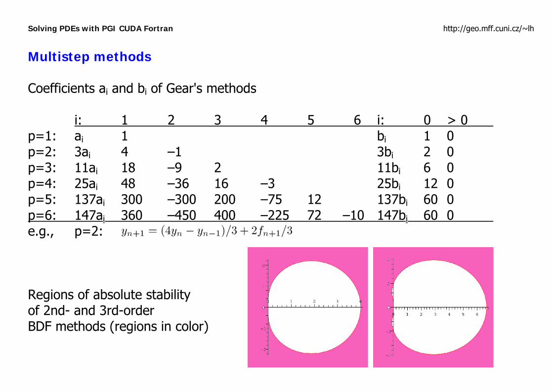
Multistep methods Coefficients ai and bi of Gear's methods i: 1 2 3 4 5 6 i: 0 > 0 p=1: ai 1 bi 1 0 p=2: 3ai 4 –1 3bi 2 0 p=3: 11ai 18 –9 2 11bi 6 0 p=4: 25ai 48 –36 16 –3 25bi 12 0 p=5: 137ai 300 –300 200 –75 12 137bi 60 0 p=6: 147ai 360 –450 400 –225 72 –10 147bi 60 0 e.g., p=2: Regions of absolute stability of 2nd- and 3rd-order BDF methods (regions in color)


On the crossroads Euler methods are extremely simple but inaccurate, too; the implicit variant is necessary when stability matters, i.e., when larger stepsize is required than a stability condition allows. Runge-Kutta explicit methods are simple and fast enough both to code and to run, as each step requires just evaluation of an explicit formula, and for many problems, they are accurate enough. However, they are explicit and stepsize is limited. Predictor-corrector implementation, including stepsize adaptivity, is rather an artwork, but it was done and can be reused from available packages. Still, stability is limited. Backward differentiation formulas, as a multistep method, share many features with predictor-corrector methods, however, for their excellent stability, they are inevitable for stiff problems.


An example: Lorenz attractor – a problem of the 2D convection in the atmosphere, mathematically simplified as much as possible – a fully deterministic system with chaotic behavior – a simplified problem: 3 ODEs for temporal evolution of 3 variables (coefficients of eigenvalue expansions of the stream function and temperature anomalies) in the 3D (phase) space

where A is a stream-function coefficient, B and C coefficients of temperature anomalies, P the Prandtl number, r=Ra/RaCR with Ra the Rayleigh number, corresponds to the size of a convection roll and is nondimensionalized time – parameters used by Lorenz (1963): P=10, r=28 and b=8/3, a sufficient time interval: 0..20


Lorenz attractor – temporal solutions roll around two fixed points (the strange attractors) along a lemniscate-shaped trajectory (like ) – physically: the boundary layer of a convection cell grows, at some point it becomes unstable, convection resumes, either as a clockwise or counterclockwise roll: chaotic behavior in a deterministic system – popular vizualization: A-B-C phase portraits


Lorenz attractor Source codes CPU: an arbitrary A-B-C point undergoes NT Runge-Kutta time steps, they are recorded and plotted CPU: NX x NY x NZ points, spread within a 3D cube, undergo NT time steps, each independent of others, only final positions of all points are recorded and plotted GPU: the previous case with one kernel GPU: the previous case, now with a smaller kernel called repeatedly Goals: a massively parallel compute-bound kernel, SP/DP execution times, avoiding kernel execution timeout, stability limits of explicit schemes


Links and references Numerical methods Ascher U. M. and Petzold L. R., Computer Methods for Ordinary Differential Equations and Differential-Algebraic Equations, SIAM, 1998 Press W. H. et al., Numerical Recipes in Fortran 77: The Art of Scientific Computing, Second Edition, Cambridge, 1992 Chapter 16.1: Runge-Kutta method Chapter 16.2: Adaptive stepsize control for Runge-Kutta Chapter 16.6: Stiff sets of equations http://www.nr.com, PDFs available at http://www.nrbook.com/a/bookfpdf.php Lorenz attractor Schubert G. et al., Mantle Convection in the Earth and Planets, Cambridge, 2001, p. 332–337 http://ebookee.org/Mantle-Convection-in-the-Earth-and-Planets_661884.html

Date post:	23-May-2018
Category:	Documents
Upload:	duongquynh
View:	215 times
Download:	0 times

Solving PDEs with PGI CUDA Fortran Part 4: Initial value...

Documents