1

Solving the Bottleneck Traveling Salesman Problem Using the Lin-Kernighan-Helsgaun Algorithm

Keld Helsgaun

E-mail: keld@ruc.dk

Computer Science Roskilde University

DK-4000 Roskilde, Denmark1

Abstract The Bottleneck Traveling Salesman Problem (BTSP) is a variation of the Traveling Sales-man Problem (TSP). The Bottleneck Traveling Salesman Problem asks for a tour in which the largest edge is as small as possible. It is well known that any BTSP instance can be solved using a TSP solver. This paper evaluates the performance of the state-of-the art TSP solver Lin-Kernighan-Helsgaun (LKH) on a large number of benchmark instances. When LKH was used as a black box, without any modifications, most instances with up to 115,475 vertices could be solved to optimality in a reasonable time. A small revision of LKH made it possible to solve BTSP instances with up to one million vertices. The pro-gram, named BLKH, is free of charge for academic and non-commercial use and can be downloaded in source code. The program is also applicable to the Maximum Scatter TSP (MSTSP), which asks for a tour in which the smallest edge is as large possible. Keywords: Bottleneck traveling salesman problem, BTSP, Maximum scatter traveling salesman problem, MSTSP, Traveling salesman problem, TSP, Lin-Kernighan Mathematics Subject Classification: 90C27, 90C35, 90C59

1. Introduction

The Bottleneck Traveling Salesman Problem (BTSP) is a variation of the Traveling Salesman Problem (TSP). The BTSP asks for a tour in which the largest edge is as small as possible. The problem has numerous applications, including transportation of perishable goods, work-force scheduling [1], and minimizing the makespan in a two-machine flowshop [2]. The BTSP is defined on a complete graph G = (V, E), where V={v1....vn} is the vertex set and E={(vi,vj) : vi, vj ∈ V, i ≠ j} is the edge set. A non-negative cost cij is associated with each edge (vi, vj). The BTSP can be stated as the problem of finding a Hamiltonian cycle whose largest edge is as small as possible. If the cost matrix C = (cij) is symmetric, i.e., cij = cji for all i, j, i≠j, the problem is called symmetric. Otherwise it is called asymmetric. Just like the TSP, the BTSP is NP-hard [3].

_________ April 2014

2

Figure 1 shows the optimal BTSP tour for usa1097, an instance consisting of 1097 cities in the adjoining 48 U.S. states, plus the District of Columbia. Its total length is 127,786,915 me-ters, and its bottleneck edge has a length of 175,360 meters. In comparison, the optimal TSP tour for this instance has a total length of 71,109,602 meters and a bottleneck edge length of 195,002 meters.

Figure 1 Optimal BTSP tour for usa1097.

It is well known that any BTSP instance can be solved using a TSP solver [3], either after transforming the BTSP instance into a standard TSP instance, or by solving the BTSP in-stance as a sequence of O(log n) standard TSP instances using Edmonds and Fulkerson’s well known threshold algorithm for bottleneck problems [4]. The first approach, however, does not have much practical value since the edge costs of the transformed instance grows exponen-tially. For this reason, the second approach has been chosen. LKH [5, 6] is a powerful local search heuristic for the TSP based on the variable depth local search of Lin and Kernighan [7]. Among its characteristics may be mentioned its use of 1-tree approximation for determining a candidate edge set, extension of the basic search step, and effective rules for directing and pruning the search. LKH is available free of charge for scien-tific and educational purposes from http://www.ruc.dk/~keld/research/LKH. The following section describes how LKH can be used as a black box to solve the BTSP.

3

2. Implementing a BTSP Solver Based on LKH Input to LKH is given in two files:

(1) A problem file in TSPLIB format [8], which contains a specification of the TSP instance to be solved. A problem may be symmetric or asymmetric. In the latter case, the problem is transformed by LKH into a symmetric one with 2n vertices.

(2) A parameter file, which contains the name of the problem file, together with some parameter values that control the solution process. Parameters that are not specified in this file are given suitable default values.

The BTSP solver, named BLKH, starts by reading the parameter file as well as the prob-lem file. A lower bound for the bottleneck cost is then computed and used for solving the BTSP. An outline of the main program (written in C) is given below.

int main(int argc, char *argv[]) { int Bottleneck, Bound, LowerBound; ReadParameters(); ReadProblem(); LowerBound = TwoMax(); if ((Bound = BBSSP(LowerBound)) > LowerBound) LowerBound = Bound; if (ProblemType == ATSP) { if ((Bound = BBSSPA(LowerBound)) > LowerBound) LowerBound = Bound; if ((Bound = BSCSSP(LowerBound)) > LowerBound) LowerBound = Bound; if ((Bound = BAP(LowerBound)) > LowerBound) LowerBound = Bound; } Bottleneck = SolveBTSP(LowerBound); }

Comments:

1. The algorithms for computing a lower bound are similar to those used by John La-Rusic et al. [9, 10].

• The TwoMax function computes the 2-Max bound. • The BBSSP function attempts to improve this bound by solving the Bottleneck

Biconnected Spanning Subgraph Problem on a symmetric cost matrix. For asymmetric instances, the following symmetric relaxation of the asymmetric cost matrix is used: c’ij = min{cij,cji}.

• The BBSSPA function attempts to improve the current lower bound for an asymmetric instance by solving the Bottleneck Biconnected Spanning Sub-graph Problem on a 2nx2n symmetric cost matrix constructed from the asym-metric nxn cost matrix using Jonker and Volgenant’s well known ATSP-to-TSP transformation [11].

• The BSCSSP function attempts to improve the current lower bound for an asymmetric instance by solving the Bottleneck Strongly Connected Spanning Subgraph Problem.

4

• Finally, the BAP function attempts to improve the current lower bound for an asymmetric instance by solving the Bottleneck Assignment Problem.

See [10] for a more precise description of these bounds. The implementation in BLKH of the lower bound algorithms for the last four bounds differs on three points from the implementation used in [10]:

(1) The current lower bound is used as an initial lower limit for the search interval.

(2) The binary search is based on interval midpoints, in contrast to [10], which uses binary search based on medians of edge costs.

(3) An initial test is made in order to decide whether it is possible to raise the current lower bound. If not, the binary search is skipped.

Computational evaluation has shown that BLKH’s strategy is efficient in both runtime and memory usage.

The four binary search algorithms follow the same pattern. Below is shown the algorithm for the BBSSP function.

int BBSSP(int Low) { int High = INT_MAX, Mid; if (Biconnected(Low)) return Low; Low++; while (Low < High) { Mid = Low + (High - Low) / 2; if (Biconnected(Mid)) High = Mid; else Low = Mid + 1; } return Low; }

3. After the lower bound has been computed, the SolveBTSP function is called in order to

solve the given BTSP instance (using LKH). The function returns the bottleneck cost of the obtained tour.

5

The implementation of the SolveBTSP function is shown below.

int SolveBTSP(int LowerBound) { int Low = LowerBound, High = INT_MAX, Bottleneck; Bottleneck = High = SolveTransformedTSP(Low, High); while (Low < High && Bottleneck != LowerBound) { int B = SolveTransformedTSP(Low, High); if (B < Bottleneck) { Bottleneck = High = B; if (High <= Low) Low = LowerBound + (High - LowerBound) / 2; } else Low += (High - Low + 1) / 2; } return Bottleneck; }

Comments:

1. As in the computation of the lower bound, binary search is also used here. The inte-gers Low and High denote the current search interval for the bottleneck cost. The algorithm differs from the one described in [10] on the following points:

• The binary search is based on interval midpoints, in contrast to [10], which

uses binary search based on medians of edge costs. • LKH is used for solving the TSPs, whereas [10] uses Concorde’s implementa-

tion of the Lin-Kernighan algorithm [12]. • Initially, an upper bound for the bottleneck cost is computed by executing

LKH. If this upper bound is equal to the lower bound, optimum has been found, and the binary search is skipped. This is advantageous, since the lower bound is often the true optimum.

• The algorithm is simpler, since the ‘shake’ strategy of [9] and [10] is not used.

2. The SolveTransformedTSP function (1) transforms the original instance into a stand-ard TSP instance according to the current values of Low and High, (2) solves this transformed instance using LKH, and (3) returns the bottleneck cost for the obtained tour. The TSP instances are constructed by the following transformation of the origi-nal cost matrix:

𝑐!!" =  

 0                                                    𝑖𝑓  𝑐!" ≤ 𝐿𝑜𝑤                                                                                                      𝑐!"                                                𝑖𝑓  𝐿𝑜𝑤 < 𝑐!" < 𝐻𝑖𝑔ℎ                                                                      

𝑐!" +𝐼𝑁𝑇_𝑀𝐴𝑋

4    𝑖𝑓  𝑐!" ≥ 𝐻𝑖𝑔ℎ                                                                                                                    

The implementation of the SolveTransformedTSP function is shown below in pseudo code.

6

int SolveTransformedTSP(int Low, int High) { Create problem file; if (High == INT_MAX) { Create parameter file with special values;

Create candidate file; } else Create parameter file based on the input parameter file; SolveTSP(); return bottleneck cost of the obtained tour; }

Comments:

1. First, the transformed cost matrix is written to a file that adheres to the TSPLIB file format [8]. A suitable parameter file is then created, and the standard TSP instance is solved by LKH.

2. When SolveTransformedTSP is called for the first time (High = INT_MAX), some special parameter values are chosen and a file that specifies candidate edges is created. The candidate edges are those edges that have a transformed cost of zero. However, since the number of such edges may be very large, pruning may be necessary in order to keep running time low. For symmetric instances, a maximum of 100 candidate edges are allowed to emanate from any vertex. If pruning for a vertex is necessary, its emanating candidate edges are chosen as the connections to its 100 nearest neighbor vertices. For asymmetric instances, the maximum number of allowable emanating candidate edges for any vertex is 1000. The special parameter values are:

CANDIDATE_FILE = <name of candidate file> GAIN23 = NO MAX_CANDIDATES = 0 MOVE_TYPE = 3 OPTIMUM = 0 RESTRICTED_SEARCH = NO SUBGRADIENT = NO SUBSEQUENT_MOVE_TYPE = 2

These parameter settings cause LKH to use non-restricted 3-opt as its basic move type (MOVE_TYPE = 3, RESTRICTED_SEARCH = NO). Non-sequential moves are not ex-plored (Gain23 = NO), and in any variable k-opt move, all submoves following the initial submove are 2-opt moves (SUBSEQUENT_MOVE_TYPE = 2). Only the edges in the candidate file will be used as candidate edges (MAX_CANDIDATES = 0), and no at-tempt is made to improve the lower bound of the TSP by subgradient optimization (SUBGRADIENT = NO). The setting OPTIMUM = 0 causes LKH to stop as soon as tour cost of zero is found. Experiments have shown that these parameter settings work very well, both when it comes to running time and tour quality.

3. For all subsequent calls of SolveTransformedTSP, the parameter settings are taken from the input parameter file given to BLKH.

4. The generated TSP instance is solved by the SolveTSP function by executing LKH as a child process (using the Standard C Library function popen()).

7

3. Improving the BTSP Solver

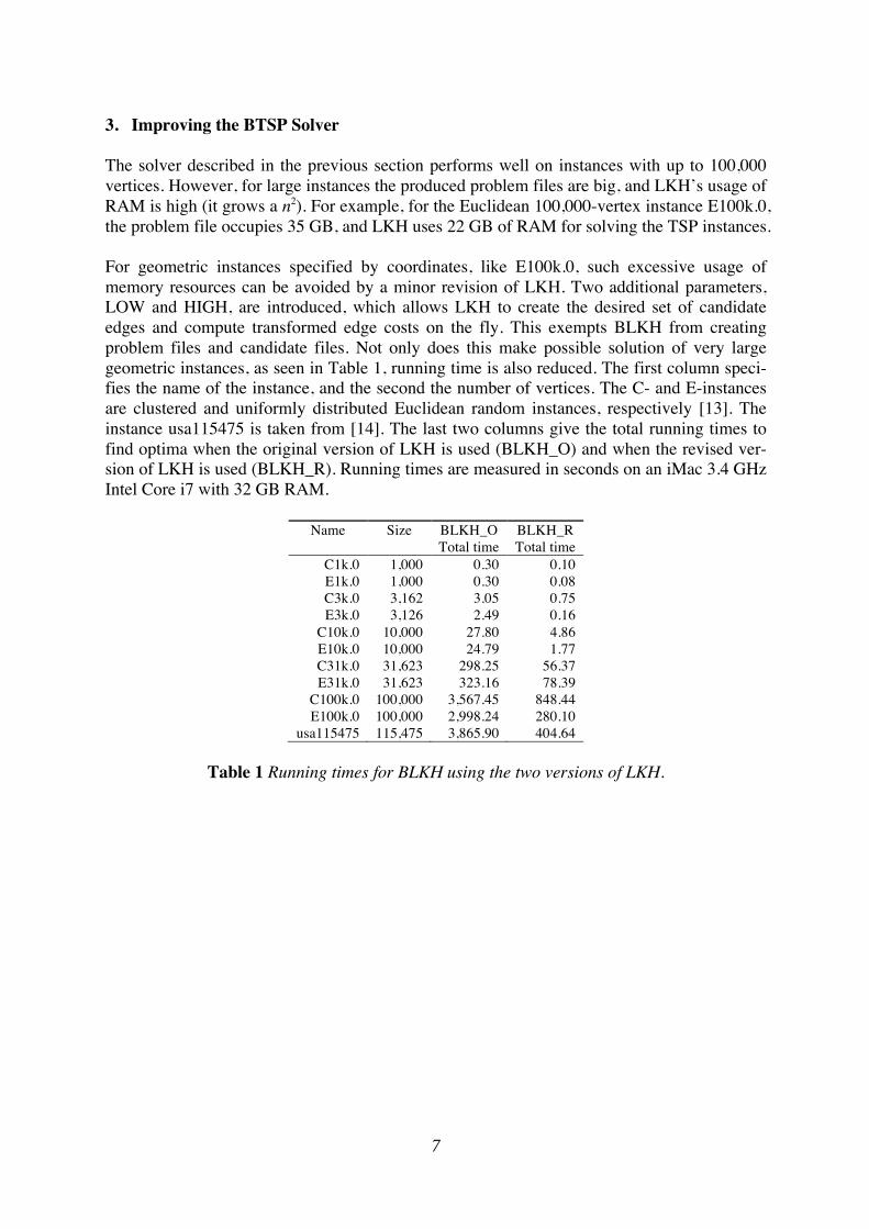
The solver described in the previous section performs well on instances with up to 100,000 vertices. However, for large instances the produced problem files are big, and LKH’s usage of RAM is high (it grows a n2). For example, for the Euclidean 100,000-vertex instance E100k.0, the problem file occupies 35 GB, and LKH uses 22 GB of RAM for solving the TSP instances. For geometric instances specified by coordinates, like E100k.0, such excessive usage of memory resources can be avoided by a minor revision of LKH. Two additional parameters, LOW and HIGH, are introduced, which allows LKH to create the desired set of candidate edges and compute transformed edge costs on the fly. This exempts BLKH from creating problem files and candidate files. Not only does this make possible solution of very large geometric instances, as seen in Table 1, running time is also reduced. The first column speci-fies the name of the instance, and the second the number of vertices. The C- and E-instances are clustered and uniformly distributed Euclidean random instances, respectively [13]. The instance usa115475 is taken from [14]. The last two columns give the total running times to find optima when the original version of LKH is used (BLKH_O) and when the revised ver-sion of LKH is used (BLKH_R). Running times are measured in seconds on an iMac 3.4 GHz Intel Core i7 with 32 GB RAM.

Name Size BLKH_O Total time

BLKH_R Total time

C1k.0 1,000 0.30 0.10 E1k.0 1,000 0.30 0.08 C3k.0 3,162 3.05 0.75 E3k.0 3,126 2.49 0.16

C10k.0 10,000 27.80 4.86 E10k.0 10,000 24.79 1.77 C31k.0 31,623 298.25 56.37 E31k.0 31,623 323.16 78.39

C100k.0 100,000 3,567.45 848.44 E100k.0 100,000 2,998.24 280.10

usa115475 115,475 3,865.90 404.64

Table 1 Running times for BLKH using the two versions of LKH.

8

4. Computational Evaluation

BLKH was coded in C and run under Linux on an iMac 3.4GHz Intel Core i7 with 32 GB RAM. The implementation is based on version 2.0.7 of LKH, which was revised as described in the previous section. The performance of BLKH has been evaluated on 339 symmetric and 352 asymmetric bench-mark instances. For all instances, the currently best known solutions were either found or im-proved. 4.1 Performance on Symmetric Instances For all symmetric instances, the following parameter settings for BLKH were chosen:

PROBLEM_FILE = TSP_INSTANCES/<instance name>.tsp INITIAL_PERIOD = 100 MAX_TRIALS = 100

MOVE_TYPE = 3 OPTIMUM = <best known cost> RUNS = 1 An explanation is given below:

PROBLEM_FILE: The symmetric test instances have been placed in the directory TSP_INSTANCES and have filename extension “.tsp”.

INITIAL_PERIOD: The candidate sets that are used in the Lin-Kernighan search pro-cess are found using a Held-Karp subgradient ascent algorithm based on minimum 1-trees [16]. The parameter specifies the length of the first period in the Held-Karp as-cent (default is n/2). MAX_TRIALS: Maximum number of trials (iterations) to be performed by the iter-ated Lin-Kernighan procedure (default is n). MOVE_TYPE: Basic k-opt move type used in the Lin-Kernighan search (default is 5). LKH offers the possibility of using higher-order and/or non-sequential move types in order to improve the solution quality. However, preliminary tests showed that 3-opt moves were sufficient for solving the symmetric benchmark instances. OPTIMUM: This parameter may be used to supply a best known solution cost. The algorithm will stop if this value is reached during the search process. RUNS: Number of runs to be performed by LKH. Set to 1, since preliminary tests showed that optimum could be found for all benchmark instances using only one run (default is 10).

9

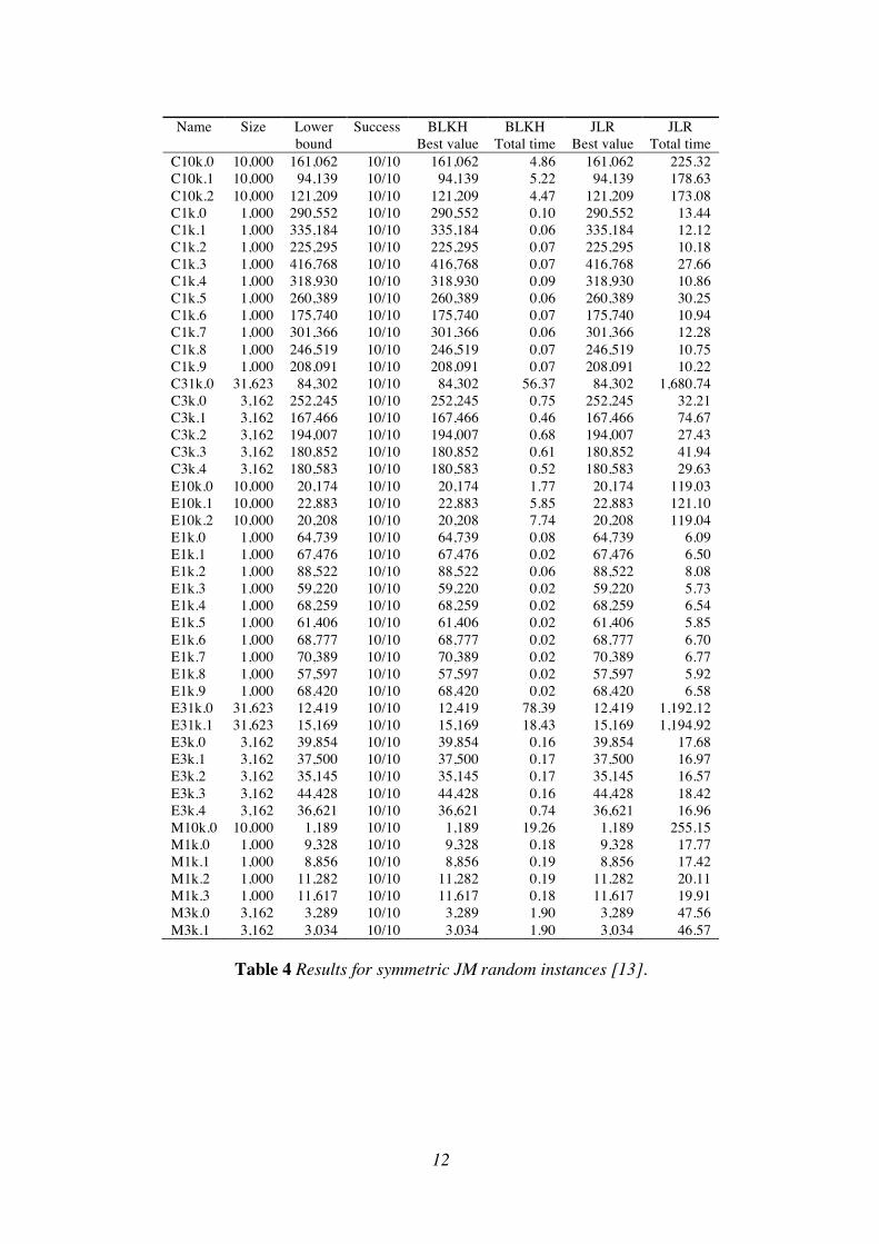
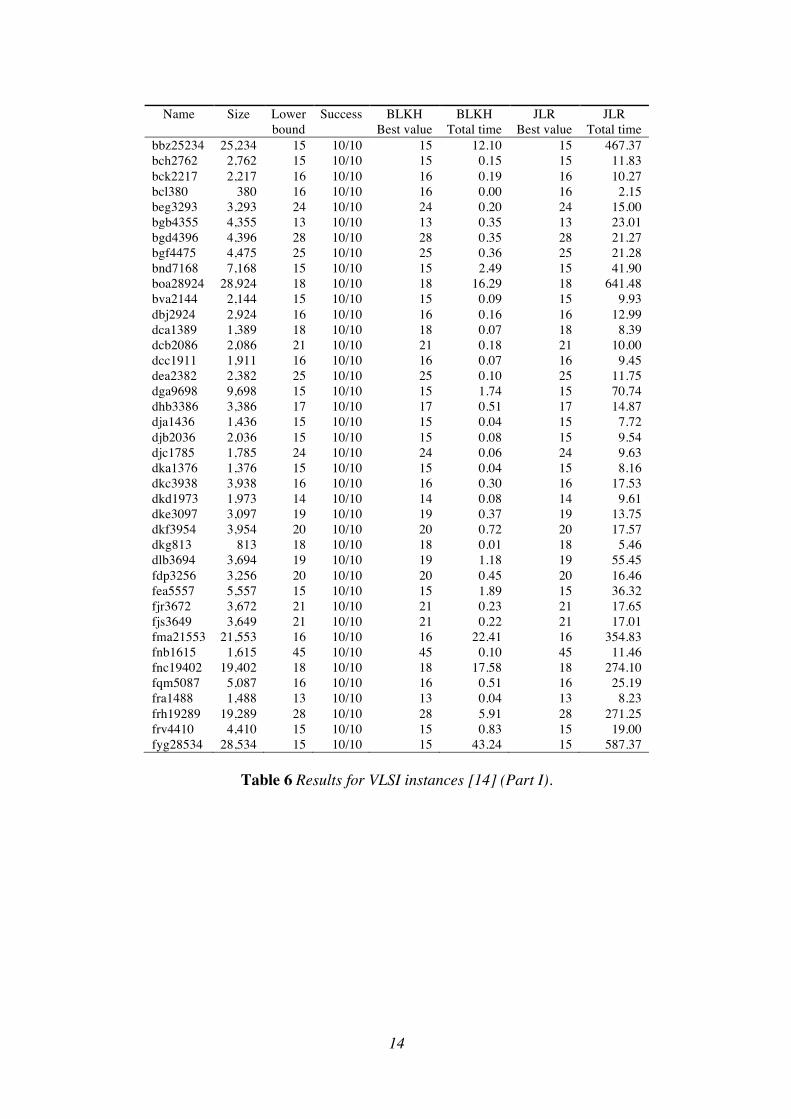
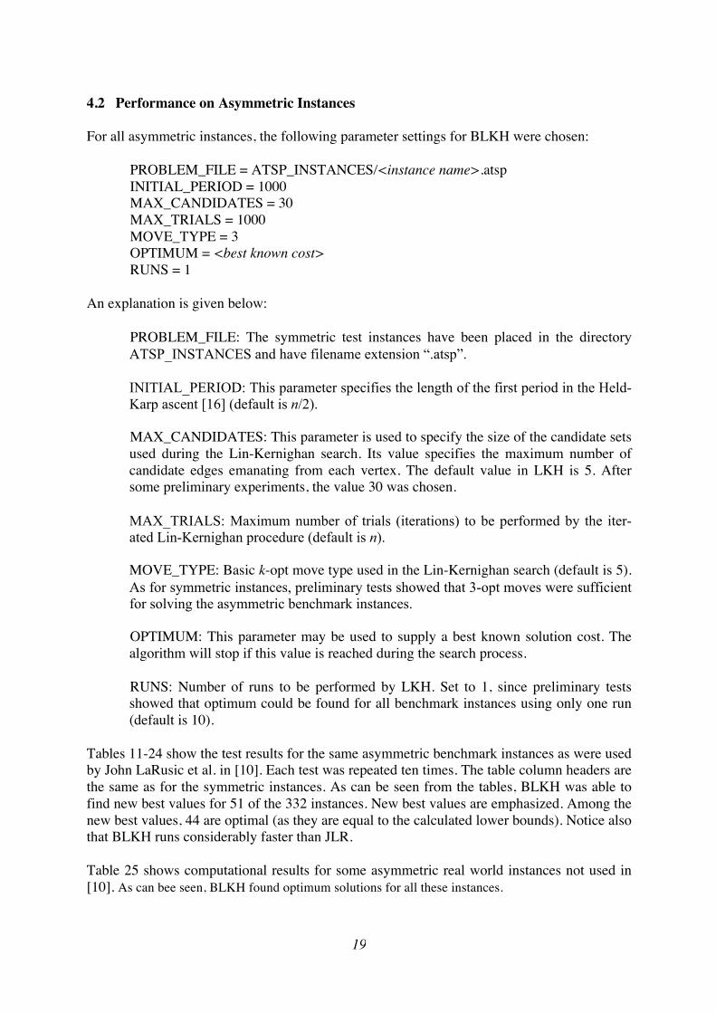
Tables 2-9 show the test results for the same symmetric benchmark instances as were used by John LaRusic et al. in [9]. Each test was repeated ten times. The column headers are as fol-lows: Name: the instance name. Size: the number of vertices. Lower bound: The lower bound (calculated by TwoMax and BBSSP). Success: The number of tests in which the best value was found. BLKH Best value: The best value found by BLKH.

BLKH Total time: The average CPU time, in seconds, used by BLKH for one test (in-cludes the time for calculating the lower bound). JLR Best value: The best value found John LaRusic et al.’s implementation (JLR). JLR Total time: The average CPU time, in seconds, used by JLR for one test (includes the time for calculating the lower bound).

As can be seen from the test results in Tables 2-9, BLKH and JLR find the same best values for these instances, but BLKH uses much less CPU time than JLR, even when it is taken into account that BLKH was run on a more powerful processor (3.4 GHz Intel i7) than the proces-sor used for running JLR (2.8 GHz Intel Xeon). That BLKH finds solutions much faster than JLR is particularly obvious from the test results for the specially constructed hard instances (Tables 8-9). Due to memory limitations, JLR was not able to solve instances with more than 31,623 verti-ces. This is not an obstacle for BLKH when using the slightly revised version of LKH. Table 10 gives the computational results for 30 instances with between 31,623 and 1,000,000 verti-ces. The column “Lower bound time” gives the time, in seconds, used to find the lower bound. All runs required less than 1 GB of RAM. As can bee seen, optimum solutions were found for all in-stances.

10

Name Size Lower bound

Success BLKH Best value

BLKH Total time

JLR Best value

JLR Total time

a280 280 20 10/10 20 0.01 20 0.92 ali535 535 3,889 10/10 3,889 0.07 3,889 7.55

att48 48 519 10/10 519 0.00 519 0.08 att532 532 229 10/10 229 0.05 229 3.85

bayg29 29 111 10/10 111 0.00 111 0.03 bays29 29 154 10/10 154 0.00 154 0.03

berlin52 52 475 10/10 475 0.00 475 0.13 bier127 127 7,486 10/10 7,486 0.00 7,486 0.78 brazil58 58 2,149 10/10 2,149 0.00 2,149 0.18

brd14051 14,051 1,306 10/10 1,306 10.42 1,306 187.73 brg180 180 30 10/10 30 0.01 30 1.00

burma14 14 418 10/10 418 0.00 418 0.01 ch130 130 142 10/10 142 0.00 142 0.42 ch150 150 93 10/10 93 0.00 93 0.38 d1291 1,291 1,289 10/10 1,289 0.04 1,289 12.49

d15112 15,112 1,370 10/10 1,370 2.80 1,370 227.86 d1655 1,655 1,476 10/10 1,476 0.07 1,476 13.44

d18512 18,512 476 10/10 476 6.70 476 304.16 d198 198 1,380 10/10 1,380 0.00 1,380 1.42

d2103 2,103 1,133 10/10 1,133 0.08 1,133 14.65 d493 493 2,008 10/10 2,008 0.01 2,008 5.34 d657 657 1,368 10/10 1,368 0.01 1,368 6.92

dantzig42 42 35 10/10 35 0.00 35 0.05 dsj1000 1,000 295,939 10/10 295,939 0.08 295,939 11.96

eil101 101 13 10/10 13 0.00 13 0.25 eil51 51 13 10/10 13 0.00 13 0.05 eil76 76 16 10/10 16 0.00 16 0.22

fl1400 1,400 530 10/10 530 0.05 530 10.58 fl1577 1,577 431 10/10 431 0.11 431 10.94 fl3795 3,795 528 10/10 528 0.27 528 22.01

fl417 417 472 10/10 472 0.01 472 5.67 fnl4461 4,461 132 10/10 132 0.42 132 23.59

fri26 26 93 10/10 93 0.00 93 0.03 gil262 262 23 10/10 23 0.00 23 0.96 gr120 120 220 10/10 220 0.00 220 0.49 gr137 137 2,132 10/10 2,132 0.01 2,132 0.69

gr17 17 282 10/10 282 0.00 282 0.01 gr202 202 2,230 10/10 2,230 0.01 2,230 1.97

gr21 21 355 10/10 355 0.00 355 0.02 gr229 229 4,027 10/10 4,027 0.01 4,027 1.85

gr24 24 108 10/10 108 0.00 108 0.02 gr431 431 4,027 10/10 4,027 0.03 4,027 5.46

gr48 48 227 10/10 227 0.00 227 0.07 gr666 666 4,264 10/10 4,264 0.06 4,264 10.33

gr96 96 2,807 10/10 2,807 0.00 2,807 0.43 hk48 48 534 10/10 534 0.00 534 0.07

kroA100 100 475 10/10 475 0.00 475 0.20 kroA150 150 392 10/10 392 0.00 392 0.34 kroA200 200 408 10/10 408 0.00 408 0.68 kroB100 100 530 10/10 530 0.00 530 0.25 kroB150 150 436 10/10 436 0.00 436 0.40 kroB200 200 344 10/10 344 0.01 344 0.55 kroC100 100 498 10/10 498 0.00 498 0.19 kroD100 100 491 10/10 491 0.00 491 0.19

Table 2 Results for symmetric TSPLIB instances [8] (Part I).

11

Name Size Lower bound

Success BLKH Best value

BLKH Total time

JLR Best value

JLR Total Time

kroE100 100 490 10/10 490 0.00 490 0.19 lin105 105 487 10/10 487 0.00 487 0.28 lin318 318 487 10/10 487 0.01 487 1.41 nrw1379 1,379 105 10/10 105 0.04 105 8.44 p654 654 1,223 10/10 1,223 0.04 1,223 5.40 pa561 561 16 10/10 16 0.03 16 3.44 pcb1173 1,173 243 10/10 243 0.03 243 8.30 pcb3038 3,038 198 10/10 198 0.42 198 13.58 pcb442 442 500 10/10 500 0.01 500 2.94 pla7397 7,397 81,438 10/10 81,438 5.52 81,438 181.79 pr1002 1,002 2,129 10/10 2,129 0.05 2,129 7.07 pr107 107 7,050 10/10 7,050 0.00 7,050 0.42 pr124 124 3,302 10/10 3,302 0.00 3,302 0.48 pr136 136 2,976 10/10 2,976 0.00 2,976 0.54 pr144 144 2,570 10/10 2,570 0.00 2,570 0.51 pr152 152 5,553 10/10 5,553 0.00 5,553 0.67 pr226 226 3,250 10/10 3,250 0.00 3,250 0.94 pr2392 2,392 481 10/10 481 0.49 481 12.03 pr264 264 4,701 10/10 4,701 0.01 4,701 1.83 pr299 299 498 10/10 498 0.02 498 2.41 pr439 439 2,384 10/10 2,384 0.00 2,384 3.07 pr76 76 3,946 10/10 3,946 0.00 3,946 0.20 rat195 195 21 10/10 21 0.00 21 0.51 rat575 575 23 10/10 23 0.01 23 2.82 rat783 783 26 10/10 26 0.01 26 5.46 rat99 99 20 10/10 20 0.00 20 0.10 rd100 100 221 10/10 221 0.00 221 0.30 rd400 400 104 10/10 104 0.01 104 1.94 rl11849 11,849 842 10/10 842 5.53 842 149.59 rl1304 1,304 1,535 10/10 1,535 0.07 1,535 9.35 rl1323 1,323 2,489 10/10 2,489 0.08 2,489 10.87 rl1889 1,889 896 10/10 896 0.18 896 9.72 rl5915 5,915 602 10/10 602 1.67 602 229.82 rl5934 5,934 896 10/10 896 1.55 896 60.29 si1032 1,032 362 10/10 362 0.15 362 21.84 si175 175 177 10/10 177 0.01 177 0.68 si535 535 227 10/10 227 0.04 227 4.35 st70 70 24 10/10 24 0.00 24 0.15 swiss42 42 67 10/10 67 0.00 67 0.06 ts225 500 1,000 10/10 1,000 0.06 1,000 2.99 tsp225 225 36 10/10 36 0.00 36 0.75 u1060 1,060 2,378 10/10 2,378 0.02 2,378 8.39 u1432 1,432 300 10/10 300 0.04 300 7.21 u159 159 800 10/10 800 0.00 800 0.52 u1817 1,817 234 10/10 234 0.06 234 8.61 u2152 2,152 105 10/10 105 0.09 105 25.66 u2319 2,319 224 10/10 224 0.09 224 10.03 u574 574 345 10/10 345 0.01 345 3.73 u724 724 170 10/10 170 0.02 170 4.00 ulysses16 16 1,504 10/10 1,504 0.00 1,504 0.01 ulysses22 22 1,504 10/10 1,504 0.00 1,504 0.03 usa13509 13,509 16,754 10/10 16,754 3.08 16,754 211.14 vm1084 1,084 998 10/10 998 0.04 998 6.91 vm1748 1,748 1,017 10/10 1,017 0.05 1,017 9.47

Table 3 Results for symmetric TSPLIB instances [8] (Part II).

12

Name Size Lower bound

Success BLKH Best value

BLKH Total time

JLR Best value

JLR Total time

C10k.0 10,000 161,062 10/10 161,062 4.86 161,062 225.32 C10k.1 10,000 94,139 10/10 94,139 5.22 94,139 178.63 C10k.2 10,000 121,209 10/10 121,209 4.47 121,209 173.08 C1k.0 1,000 290,552 10/10 290,552 0.10 290,552 13.44 C1k.1 1,000 335,184 10/10 335,184 0.06 335,184 12.12 C1k.2 1,000 225,295 10/10 225,295 0.07 225,295 10.18 C1k.3 1,000 416,768 10/10 416,768 0.07 416,768 27.66 C1k.4 1,000 318,930 10/10 318,930 0.09 318,930 10.86 C1k.5 1,000 260,389 10/10 260,389 0.06 260,389 30.25 C1k.6 1,000 175,740 10/10 175,740 0.07 175,740 10.94 C1k.7 1,000 301,366 10/10 301,366 0.06 301,366 12.28 C1k.8 1,000 246,519 10/10 246,519 0.07 246,519 10.75 C1k.9 1,000 208,091 10/10 208,091 0.07 208,091 10.22 C31k.0 31,623 84,302 10/10 84,302 56.37 84,302 1,680.74 C3k.0 3,162 252,245 10/10 252,245 0.75 252,245 32.21 C3k.1 3,162 167,466 10/10 167,466 0.46 167,466 74.67 C3k.2 3,162 194,007 10/10 194,007 0.68 194,007 27.43 C3k.3 3,162 180,852 10/10 180,852 0.61 180,852 41.94 C3k.4 3,162 180,583 10/10 180,583 0.52 180,583 29.63 E10k.0 10,000 20,174 10/10 20,174 1.77 20,174 119.03 E10k.1 10,000 22,883 10/10 22,883 5.85 22,883 121.10 E10k.2 10,000 20,208 10/10 20,208 7.74 20,208 119.04 E1k.0 1,000 64,739 10/10 64,739 0.08 64,739 6.09 E1k.1 1,000 67,476 10/10 67,476 0.02 67,476 6.50 E1k.2 1,000 88,522 10/10 88,522 0.06 88,522 8.08 E1k.3 1,000 59,220 10/10 59,220 0.02 59,220 5.73 E1k.4 1,000 68,259 10/10 68,259 0.02 68,259 6.54 E1k.5 1,000 61,406 10/10 61,406 0.02 61,406 5.85 E1k.6 1,000 68,777 10/10 68,777 0.02 68,777 6.70 E1k.7 1,000 70,389 10/10 70,389 0.02 70,389 6.77 E1k.8 1,000 57,597 10/10 57,597 0.02 57,597 5.92 E1k.9 1,000 68,420 10/10 68,420 0.02 68,420 6.58 E31k.0 31,623 12,419 10/10 12,419 78.39 12,419 1,192.12 E31k.1 31,623 15,169 10/10 15,169 18.43 15,169 1,194.92 E3k.0 3,162 39,854 10/10 39,854 0.16 39,854 17.68 E3k.1 3,162 37,500 10/10 37,500 0.17 37,500 16.97 E3k.2 3,162 35,145 10/10 35,145 0.17 35,145 16.57 E3k.3 3,162 44,428 10/10 44,428 0.16 44,428 18.42 E3k.4 3,162 36,621 10/10 36,621 0.74 36,621 16.96 M10k.0 10,000 1,189 10/10 1,189 19.26 1,189 255.15 M1k.0 1,000 9,328 10/10 9,328 0.18 9,328 17.77 M1k.1 1,000 8,856 10/10 8,856 0.19 8,856 17.42 M1k.2 1,000 11,282 10/10 11,282 0.19 11,282 20.11 M1k.3 1,000 11,617 10/10 11,617 0.18 11,617 19.91 M3k.0 3,162 3,289 10/10 3,289 1.90 3,289 47.56 M3k.1 3,162 3,034 10/10 3,034 1.90 3,034 46.57

Table 4 Results for symmetric JM random instances [13].

13

Name Size Lower bound

Success BLKH Best value

BLKH Total time

JLR Best value

JLR Total time

ar9152 9,152 4,871 10/10 4,871 1.77 4,871 102.02 ca4663 4,663 13,768 10/10 13,768 1.21 13,768 35.18 dj89 89 437 10/10 437 0.00 437 0.29 eg7146 7,146 2,150 10/10 2,150 2.27 2,150 65.86 ei8246 8,246 124 10/10 124 1.44 124 65.69 fi10639 10,639 768 10/10 768 1.73 768 106.56 gr9882 9,882 1,399 10/10 1,399 1.99 1,399 97.15 ho14473 14,473 440 10/10 440 7.66 440 208.38 it16862 16,862 1,499 10/10 1,499 10.71 1,499 431.88 ja9847 9,847 6,413 10/10 6,413 4.71 6,413 101.17 kz9976 9,976 1,602 10/10 1,602 1.89 1,602 103.94 lu980 980 44 10/10 44 0.02 44 5.97 mo14185 14,185 939 10/10 939 10.88 939 180.20 mu1979 1,979 1,153 10/10 1,153 0.09 1,153 14.10 nu3496 3,496 650 10/10 650 0.35 650 24.84 pm8079 8,079 331 10/10 331 2.39 331 75.56 qa194 194 370 10/10 370 0.00 370 1.13 rw1621 1,621 150 10/10 150 0.09 150 11.46 sw24978 24,978 1,068 10/10 1,068 37.19 1,068 8,270.68 tz6117 6,117 486 10/10 486 0.74 486 40.26 uy734 734 389 10/10 389 0.04 389 5.04 vm22775 22,775 388 10/10 388 9.94 388 477.76 wi29 29 2,250 10/10 2,250 0.00 2,250 0.02 ym7663 7,663 3,113 10/10 3,113 2.74 3,113 66.67 zi929 929 887 10/10 887 0.02 887 8.12

Table 5 Results for National TSP instances [14].

14

Name Size Lower bound

Success BLKH Best value

BLKH Total time

JLR Best value

JLR Total time

bbz25234 25,234 15 10/10 15 12.10 15 467.37 bch2762 2,762 15 10/10 15 0.15 15 11.83 bck2217 2,217 16 10/10 16 0.19 16 10.27 bcl380 380 16 10/10 16 0.00 16 2.15 beg3293 3,293 24 10/10 24 0.20 24 15.00 bgb4355 4,355 13 10/10 13 0.35 13 23.01 bgd4396 4,396 28 10/10 28 0.35 28 21.27 bgf4475 4,475 25 10/10 25 0.36 25 21.28 bnd7168 7,168 15 10/10 15 2.49 15 41.90 boa28924 28,924 18 10/10 18 16.29 18 641.48 bva2144 2,144 15 10/10 15 0.09 15 9.93 dbj2924 2,924 16 10/10 16 0.16 16 12.99 dca1389 1,389 18 10/10 18 0.07 18 8.39 dcb2086 2,086 21 10/10 21 0.18 21 10.00 dcc1911 1,911 16 10/10 16 0.07 16 9.45 dea2382 2,382 25 10/10 25 0.10 25 11.75 dga9698 9,698 15 10/10 15 1.74 15 70.74 dhb3386 3,386 17 10/10 17 0.51 17 14.87 dja1436 1,436 15 10/10 15 0.04 15 7.72 djb2036 2,036 15 10/10 15 0.08 15 9.54 djc1785 1,785 24 10/10 24 0.06 24 9.63 dka1376 1,376 15 10/10 15 0.04 15 8.16 dkc3938 3,938 16 10/10 16 0.30 16 17.53 dkd1973 1,973 14 10/10 14 0.08 14 9.61 dke3097 3,097 19 10/10 19 0.37 19 13.75 dkf3954 3,954 20 10/10 20 0.72 20 17.57 dkg813 813 18 10/10 18 0.01 18 5.46 dlb3694 3,694 19 10/10 19 1.18 19 55.45 fdp3256 3,256 20 10/10 20 0.45 20 16.46 fea5557 5,557 15 10/10 15 1.89 15 36.32 fjr3672 3,672 21 10/10 21 0.23 21 17.65 fjs3649 3,649 21 10/10 21 0.22 21 17.01 fma21553 21,553 16 10/10 16 22.41 16 354.83 fnb1615 1,615 45 10/10 45 0.10 45 11.46 fnc19402 19,402 18 10/10 18 17.58 18 274.10 fqm5087 5,087 16 10/10 16 0.51 16 25.19 fra1488 1,488 13 10/10 13 0.04 13 8.23 frh19289 19,289 28 10/10 28 5.91 28 271.25 frv4410 4,410 15 10/10 15 0.83 15 19.00 fyg28534 28,534 15 10/10 15 43.24 15 587.37

Table 6 Results for VLSI instances [14] (Part I).

15

Name Size Lower bound

Success BLKH Best value

BLKH Total time

JLR Best value

JLR Total time

icw1483 1,483 21 10/10 21 0.08 21 9.07 icx28698 28,698 18 10/10 18 16.39 18 594.93 ida8197 8,197 14 10/10 14 1.24 14 55.20 ido21215 21,215 16 10/10 16 7.50 16 345.75 ird29514 29,514 16 10/10 16 17.70 16 629.35 irw2802 2,802 15 10/10 15 0.33 15 12.52 irx28268 28,268 15 10/10 15 36.75 15 575.07 lap7454 7,454 16 10/10 16 1.02 16 45.54 ley2323 2,323 27 10/10 27 0.19 27 11.47 lim963 963 13 10/10 13 0.04 13 6.98 lsb22777 22,777 23 10/10 23 26.73 23 374.12 lsm2854 2,854 19 10/10 19 0.15 19 12.85 lsn3119 3,119 16 10/10 16 0.18 16 13.89 lta3140 3,140 17 10/10 17 0.19 17 13.95 ltb3729 3,729 13 10/10 13 0.31 13 17.97 mlt2597 2,597 21 10/10 21 0.12 21 11.98 pbd984 984 13 10/10 13 0.02 13 7.17 pbk411 411 14 10/10 14 0.01 14 2.54 pbl395 395 13 10/10 13 0.01 13 2.31 pbm436 436 15 10/10 15 0.01 15 2.70 pbn423 423 14 10/10 14 0.01 14 2.46 pds2566 2,566 15 10/10 15 0.26 15 11.14 pia3056 3,056 15 10/10 15 0.18 15 13.57 pjh17845 17,845 14 10/10 14 5.07 14 231.96 pka379 379 11 10/10 11 0.00 11 1.75 pma343 343 15 10/10 15 0.00 15 1.77 rbu737 737 13 10/10 13 0.02 13 4.62 rbv1583 1,583 18 10/10 18 0.11 18 8.68 rbw2481 2,481 27 10/10 27 0.23 27 11.96 rbx711 711 15 10/10 15 0.01 15 4.35 rby1599 1,599 18 10/10 18 0.12 18 9.58 xia16928 16,928 15 10/10 15 4.59 15 310.45 xit1083 1,083 11 10/10 11 0.02 11 6.46 xmc10150 10,150 17 10/10 17 1.56 17 239.83 xpr2308 2,308 14 10/10 14 0.10 14 10.09 xqc2175 2,175 15 10/10 15 0.20 15 10.18

Table 7 Results for VLSI instances [14] (Part II).

16

Beta Gamma r Seed Success Lower bound

BLKH Best value

BLKH Total time

JLR Best value

JLR Total time

500 5,000 125 6,125 10/10 29 525 4.33 525 6,190.58 500 5,000 250 6,250 10/10 17 17 0.03 17 5.94 500 5,000 375 6,375 10/10 35 524 6.43 524 5,491.03 500 7,500 125 8,625 10/10 31 538 5.82 538 5,709.70 500 7,500 250 8,750 10/10 22 22 0.03 22 5.77 500 7,500 375 8,875 10/10 36 537 10.47 537 5,272.00 500 10,000 125 11,125 10/10 53 547 13.68 547 4,749.93 500 10,000 250 11,250 10/10 20 20 0.03 20 5.98 500 10,000 375 11,375 10/10 30 551 7.24 551 5,471.06

1,000 5,000 125 6,625 10/10 56 1,022 4.66 1,022 6,573.59 1,000 5,000 250 6,750 10/10 26 26 0.03 26 5.60 1,000 5,000 375 6,875 10/10 73 1,019 8.41 1,019 6,061.48 1,000 7,500 125 9,125 10/10 59 1,031 5.66 1,031 6,697.39 1,000 7,500 250 9,250 10/10 40 40 0.03 40 5.99 1,000 7,500 375 9,375 10/10 55 1,034 5.41 1,034 6,396.32 1,000 10,000 125 11,625 10/10 70 1,052 12.55 1,052 5,721.51 1,000 10,000 250 11,750 10/10 34 34 0.03 34 5.98 1,000 10,000 375 11,875 10/10 99 1,047 13.50 1,047 5,336.26 2,500 5,000 125 8,125 10/10 175 2,514 6.95 2,514 6,897.77 2,500 5,000 250 8,250 10/10 88 88 0.04 88 6.18 2,500 5,000 375 8,375 10/10 156 2,513 6.21 2,513 7,088.92 2,500 7,500 125 10,625 10/10 174 2,530 7.71 2,530 6,446.26 2,500 7,500 250 10,750 10/10 106 106 0.04 106 5.79 2,500 7,500 375 10,875 10/10 170 2,528 7.38 2,528 6,493.24 2,500 10,000 125 13,125 10/10 171 2,534 9.43 2,534 6,874.99 2,500 10,000 250 13,250 10/10 83 83 0.04 83 6.11 2,500 10,000 375 13,375 10/10 161 2,536 6.32 2,536 6,539.55

Table 8 Results for hard instances with n = 500 [9].

17

Beta Gamma r Seed Success Lower bound

BLKH Best value

BLKH Total time

JLR Best value

JLR Total time

500 5,000 625 8,625 10/10 7 505 189.12 505 24,305.76 500 5,000 1,250 9,250 10/10 4 4 0.81 4 32.01 500 5,000 1,875 9,875 10/10 9 505 306.22 505 21,989.61 500 7,500 625 11,125 10/10 9 508 239.56 508 23,334.92 500 7,500 1,250 11,750 10/10 4 4 0.81 4 32.55 500 7,500 1,875 12,375 10/10 8 507 192.47 507 22,762.23 500 10,000 625 13,625 10/10 6 510 179.83 510 23,854.55 500 10,000 1250 14,250 10/10 4 4 0.81 4 32.44 500 10,000 1875 14,875 10/10 7 510 176.55 510 23,708.87

1,000 5,000 625 9,125 10/10 16 1,005 171.32 1,005 25,242.82 1,000 5,000 1,250 9,750 10/10 6 6 0.82 6 35.85 1,000 5,000 1,875 10,375 10/10 16 1,005 200.40 1,005 25,255.14 1,000 7,500 625 11,625 10/10 14 1,007 191.53 1,007 25,724.98 1,000 7,500 1,250 12,250 10/10 8 8 0.85 8 34.84 1,000 7,500 1,875 12,875 10/10 16 1,007 268.91 1,007 24,531.80 1,000 10,000 625 14,125 10/10 17 1,009 256.42 1,009 23,909.13 1,000 10,000 1,250 14,750 10/10 6 6 0.84 6 35.28 1,000 10,000 1,875 15,375 10/10 17 1,009 253.63 1,009 24,152.90 2,500 5,000 625 10,625 10/10 39 2,503 205.60 2,503 27,607.44 2,500 5,000 1,250 11,250 10/10 21 21 0.89 21 33.17 2,500 5,000 1,875 11,875 10/10 40 2,503 174.84 2,503 26,995.48 2,500 7,500 625 13,125 10/10 46 2,506 256.41 2,506 25,895.66 2,500 7,500 1,250 13,750 10/10 22 22 0.89 22 36.52 2,500 7,500 1,875 14,375 10/10 35 2,506 196.41 2,506 27,706.35 2,500 10,000 625 15,625 10/10 38 2,509 264.72 2,509 26,657.82 2,500 10,000 1,250 16,250 10/10 17 17 1.01 17 37.25 2,500 10,000 1,875 16,875 10/10 37 2,508 273.14 2,508 26,699.86

Table 9 Results for hard instances with n = 2,500 [9].

18

Name Size Lower bound

Lower bound time

BLKH Best value

BLKH Total time

pla33810 33,810 30,266 96.64 30,266 119.46 pla85900 85,900 51,006 723.77 51,006 953.31 ch71009 71,009 1,509 345.69 1,509 454.82 usa115475 115,475 1,110 115.80 1,110 404.64 C31k.1 31,623 65,079 46.16 65,079 68.61 C100k.0 100,000 44,745 560.56 44,745 848.44 C316k.0 316,228 23,159 8,855.63 23,159 11,137.78 E100k.0 100,000 7,169 73.84 7,169 280.10 E316k.0 316,228 4,382 960.17 4,382 3,203.02 E1M.0 1,000,000 2,396 10,605.88 2,396 33,543.05 ara238025 238,025 161 6,004.04 161 7,304.01 bby34656 34,656 18 8.67 18 26.02 bna56769 56,769 16 145.53 16 201.92 dan59296 59,296 23 30.67 23 93.19 fht47608 47,608 16 93.52 16 130.93 fna52057 52,057 16 119.42 16 165.59 fry33203 33,203 20 45.03 20 60.43 ics39603 39,603 18 62.29 18 86.10 lra498378 498,378 1,341 27,596.81 1,341 34,519.57 lrb744710 744,710 86 54,586.40 86 67,586.45 pbh30440 30,440 26 6.15 26 18.52 rbz43748 43,748 14 82.55 14 112.90 sra104815 104,815 194 662.00 194 909.87 xib32892 32,892 19 41.43 19 56.39 mona-lisa100K 100,000 340 36.74 340 241.80 vangogh120K 120,000 218 78.84 218 379.79 venus140K 140,000 185 120.95 185 537.75 pareja160K 160,000 283 133.94 283 687.35 courbet180K 180,000 230 194.70 230 900.96 earring200K 200,000 394 214.12 394 1,096.22

Table 10 Results for very large symmetric instances [8][13][14].

19

4.2 Performance on Asymmetric Instances

For all asymmetric instances, the following parameter settings for BLKH were chosen:

PROBLEM_FILE = ATSP_INSTANCES/<instance name>.atsp INITIAL_PERIOD = 1000 MAX_CANDIDATES = 30 MAX_TRIALS = 1000

MOVE_TYPE = 3 OPTIMUM = <best known cost> RUNS = 1 An explanation is given below:

PROBLEM_FILE: The symmetric test instances have been placed in the directory ATSP_INSTANCES and have filename extension “.atsp”.

INITIAL_PERIOD: This parameter specifies the length of the first period in the Held-Karp ascent [16] (default is n/2). MAX_CANDIDATES: This parameter is used to specify the size of the candidate sets used during the Lin-Kernighan search. Its value specifies the maximum number of candidate edges emanating from each vertex. The default value in LKH is 5. After some preliminary experiments, the value 30 was chosen. MAX_TRIALS: Maximum number of trials (iterations) to be performed by the iter-ated Lin-Kernighan procedure (default is n). MOVE_TYPE: Basic k-opt move type used in the Lin-Kernighan search (default is 5). As for symmetric instances, preliminary tests showed that 3-opt moves were sufficient for solving the asymmetric benchmark instances. OPTIMUM: This parameter may be used to supply a best known solution cost. The algorithm will stop if this value is reached during the search process. RUNS: Number of runs to be performed by LKH. Set to 1, since preliminary tests showed that optimum could be found for all benchmark instances using only one run (default is 10).

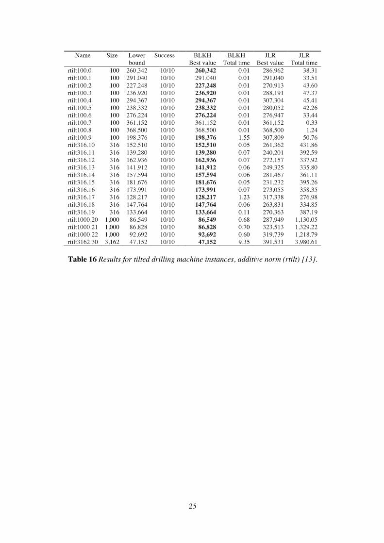
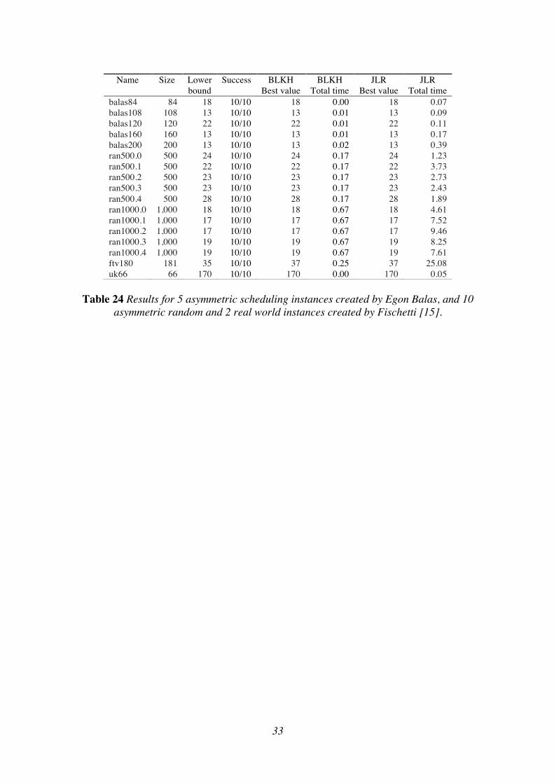
Tables 11-24 show the test results for the same asymmetric benchmark instances as were used by John LaRusic et al. in [10]. Each test was repeated ten times. The table column headers are the same as for the symmetric instances. As can be seen from the tables, BLKH was able to find new best values for 51 of the 332 instances. New best values are emphasized. Among the new best values, 44 are optimal (as they are equal to the calculated lower bounds). Notice also that BLKH runs considerably faster than JLR. Table 25 shows computational results for some asymmetric real world instances not used in [10]. As can bee seen, BLKH found optimum solutions for all these instances.

20

Name Size Lower bound

Success BLKH Best value

BLKH Total time

JLR Best value

JLR Total time

amat100.0 100 50,981 10/10 50,981 0.01 50,981 0.13 amat100.1 100 26,551 10/10 26,551 0.01 50,821 0.16 amat100.2 100 50,821 10/10 50,821 0.01 63,674 0.13 amat100.3 100 21,695 10/10 21,695 0.01 62,994 0.17 amat100.4 100 63,674 10/10 63,674 0.02 55,534 0.15 amat100.5 100 17,539 10/10 17,539 0.01 44,548 0.15 amat100.6 100 62,994 10/10 62,994 0.01 72,650 0.15 amat100.7 100 19,952 10/10 19,952 0.01 59,291 0.15 amat100.8 100 55,534 10/10 55,534 0.01 55,462 0.13 amat100.9 100 20,779 10/10 20,779 0.01 49,928 0.13 amat316.10 316 17,207 10/10 17,207 0.04 21,896 0.98 amat316.11 316 59,291 10/10 59,291 0.10 20,451 1.25 amat316.12 316 43,608 10/10 43,608 0.04 26,551 0.88 amat316.13 316 55,462 10/10 55,462 0.07 21,695 1.04 amat316.14 316 9,978 10/10 9,978 0.04 17,539 2.64 amat316.15 316 49,928 10/10 49,928 0.04 19,952 2.07 amat316.16 316 10,624 10/10 10,624 0.04 20,779 1.18 amat316.17 316 21,896 10/10 21,896 0.04 26,165 0.95 amat316.18 316 6,715 10/10 6,715 0.04 17,207 1.71 amat316.19 316 20,451 10/10 20,451 0.04 43,608 2.36 amat1000.20 1,000 44,548 10/10 44,548 0.39 9,978 15.35 amat1000.21 1,000 26,165 10/10 26,165 0.39 10,624 15.81 amat1000.22 1,000 72,650 10/10 72,650 0.40 6,715 29.15 amat3162.30 3,162 2,985 10/10 2,985 3.99 47,237 5,760.72

Table 11 Results for random asymmetric instances (amat) [13].

21

Name Size Lower bound

Success BLKH Best value

BLKH Total time

JLR Best value

JLR Total time

coin100.0 100 253 10/10 253 0.01 253 14.49 coin100.1 100 219 10/10 219 0.01 219 18.85 coin100.2 100 203 10/10 203 0.23 203 16.18 coin100.3 100 232 10/10 232 0.01 232 20.84 coin100.4 100 214 10/10 214 0.01 214 0.16 coin100.5 100 244 10/10 244 0.01 244 18.60 coin100.6 100 239 10/10 239 0.00 239 9.68 coin100.7 100 265 10/10 265 0.00 265 20.47 coin100.8 100 198 10/10 198 0.12 198 15.54 coin100.9 100 243 10/10 243 0.01 243 21.38 coin316.10 316 227 10/10 227 0.04 227 82.78 coin316.11 316 238 10/10 238 0.04 238 87.09 coin316.12 316 225 10/10 225 0.05 225 72.60 coin316.13 316 245 10/10 245 0.14 245 66.07 coin316.14 316 278 10/10 278 0.03 278 88.84 coin316.15 316 282 10/10 282 0.04 282 56.75 coin316.16 316 243 10/10 243 0.06 243 47.92 coin316.17 316 277 10/10 277 0.03 277 88.05 coin316.18 316 277 10/10 277 0.04 277 66.54 coin316.19 316 259 10/10 259 0.03 259 0.53 coin1000.20 1,000 278 10/10 278 0.34 278 341.00 coin1000.21 1,000 327 10/10 327 0.32 327 422.52 coin1000.22 1,000 245 10/10 245 0.33 249 279.33 coin3162.30 3,162 260 10/10 260 3.85 649 4,075.57

Table 12 Results for pay phone collection instances (coin) [13].

22

Name Size Lower bound

Success BLKH Best value

BLKH Total time

JLR Best value

JLR Total time

crane100.0 100 173,390 10/10 173,390 0.01 173,390 0.12 crane100.1 100 152,923 10/10 152,923 0.14 180,146 30.65 crane100.2 100 214,843 10/10 214,843 0.01 214,843 0.14 crane100.3 100 145,622 10/10 145,622 0.01 145,622 0.28 crane100.4 100 171,484 10/10 171,484 0.01 171,484 0.26 crane100.5 100 205,739 10/10 205,739 0.01 205,739 0.12 crane100.6 100 185,071 10/10 185,071 0.01 185,071 0.17 crane100.7 100 200,173 10/10 200,173 0.01 200,173 0.12 crane100.8 100 205,258 10/10 205,258 0.01 205,258 0.18 crane100.9 100 192,987 10/10 192,987 0.01 192,987 23.40 crane316.10 316 119,345 10/10 119,345 0.99 120,333 136.68 crane316.11 316 108,045 10/10 108,045 0.04 108,045 1.08 crane316.12 316 132,750 10/10 132,750 0.04 132,750 2.34 crane316.13 316 102,898 10/10 102,898 0.05 102,898 0.95 crane316.14 316 145,963 10/10 145,963 0.04 145,963 0.73 crane316.15 316 128,548 10/10 128,548 0.05 128,548 192.00 crane316.16 316 111,939 10/10 111,939 0.04 111,939 1.71 crane316.17 316 102,571 10/10 102,571 0.04 102,571 1.42 crane316.18 316 106,821 10/10 106,821 0.05 106,821 1.92 crane316.19 316 133,399 10/10 133,399 0.04 133,399 0.86 crane1000.20 1,000 56,343 10/10 56,343 0.42 56,343 19.44 crane1000.21 1,000 61,720 10/10 64,450 28.83 64,450 722.66 crane1000.22 1,000 58,091 10/10 58,466 4.01 58,466 489.04 crane3162.30 3,162 41,751 10/10 41,751 4.31 76,894 6,234.88

Table 13 Results for random Euclidean stacker crane instances (crane) [13].

23

Name Size Lower bound

Success BLKH Best value

BLKH Total time

JLR Best value

JLR Total time

disk100.0 100 508,034 10/10 508,034 0.01 508,034 0.12 disk100.1 100 473,495 10/10 473,495 0.01 473,495 0.10 disk100.2 100 382,677 10/10 382,677 0.11 386,809 10.39 disk100.3 100 453,657 10/10 453,657 0.01 453,657 0.15 disk100.4 100 415,696 10/10 415,696 0.01 415,696 0.19 disk100.5 100 553,069 10/10 553,069 0.01 553,069 0.21 disk100.6 100 432,563 10/10 432,563 0.01 432,563 0.13 disk100.7 100 550,543 10/10 550,543 0.01 550,543 0.16 disk100.8 100 396,159 10/10 396,159 0.01 396,159 0.40 disk100.9 100 426,697 10/10 426,697 0.01 426,697 0.22 disk316.10 316 309,801 10/10 309,801 0.05 309,801 0.82 disk316.11 316 259,308 10/10 259,308 0.08 259,308 1.33 disk316.12 316 273,516 10/10 273,516 0.05 273,516 1.41 disk316.13 316 236,394 10/10 236,394 0.18 236,394 32.21 disk316.14 316 226,920 10/10 226,920 0.05 226,920 2.64 disk316.15 316 271,724 10/10 271,724 0.05 271,724 1.50 disk316.16 316 249,590 10/10 249,590 0.15 249,590 7.44 disk316.17 316 305,813 10/10 305,813 0.05 305,813 1.01 disk316.18 316 246,356 10/10 246,356 0.19 246,356 1.37 disk316.19 316 320,680 10/10 320,680 0.18 320,680 1.16 disk1000.20 1,000 190,741 10/10 190,741 0.46 190,741 975.74 disk1000.21 1,000 190,665 10/10 190,665 0.45 190,665 746.68 disk1000.22 1,000 171,509 10/10 171,509 3.79 195,825 1,537.19 disk3162.30 3,162 114,028 10/10 114,028 8.52 275,891 5,957.56

Table 14 Results for disk drive instances (disk) [13].

24

Name Size Lower bound

Success BLKH Best value

BLKH Total time

JLR Best value

JLR Total time

rect100.0 100 223,717 10/10 223,717 0.01 223,717 12.40 rect100.1 100 296,349 10/10 296,349 0.01 296,349 28.72 rect100.2 100 198,319 10/10 198,319 0.01 198,319 22.94 rect100.3 100 252,297 10/10 252,297 0.01 252,297 24.45 rect100.4 100 246,494 10/10 246,494 0.01 246,494 27.80 rect100.5 100 270,406 10/10 270,406 0.01 270,406 22.01 rect100.6 100 226,069 10/10 226,069 0.01 226,069 18.40 rect100.7 100 245,457 10/10 245,457 0.01 245,457 21.60 rect100.8 100 259,347 10/10 259,347 0.01 259,347 27.80 rect100.9 100 199,114 10/10 199,114 0.24 200,000 22.88 rect316.10 316 160,358 10/10 160,358 0.04 160,358 168.87 rect316.11 316 133,083 10/10 133,083 0.07 133,083 121.94 rect316.12 316 143,209 10/10 143,209 0.05 143,209 134.99 rect316.13 316 116,995 10/10 116,995 0.05 116,995 104.04 rect316.14 316 140,437 10/10 140,437 0.05 140,437 158.32 rect316.15 316 144,858 10/10 144,858 0.05 144,858 118.90 rect316.16 316 142,029 10/10 142,029 0.05 142,029 110.67 rect316.17 316 121,054 10/10 121,054 0.05 121,054 110.10 rect316.18 316 166,616 10/10 166,616 0.05 166,616 217.73 rect316.19 316 142,134 10/10 142,134 0.05 142,134 151.49 rect1000.20 1,000 88,925 10/10 88,925 0.44 88,925 521.58 rect1000.21 1,000 82,241 10/10 82,241 0.45 82,241 543.19 rect1000.22 1,000 73,643 10/10 73,643 0.47 73,643 398.07 rect3162.30 3,162 47,063 10/10 47,063 5.21 123,706 5,241.82

Table 15 Results for random two-dimensional rectilinear instances (rect) [13].

25

Name Size Lower bound

Success BLKH Best value

BLKH Total time

JLR Best value

JLR Total time

rtilt100.0 100 260,342 10/10 260,342 0.01 286,962 38.31 rtilt100.1 100 291,040 10/10 291,040 0.01 291,040 33.51 rtilt100.2 100 227,248 10/10 227,248 0.01 270,913 43.60 rtilt100.3 100 236,920 10/10 236,920 0.01 288,191 47.37 rtilt100.4 100 294,367 10/10 294,367 0.01 307,304 45.41 rtilt100.5 100 238,332 10/10 238,332 0.01 280,052 42.26 rtilt100.6 100 276,224 10/10 276,224 0.01 276,947 33.44 rtilt100.7 100 361,152 10/10 361,152 0.01 361,152 0.33 rtilt100.8 100 368,500 10/10 368,500 0.01 368,500 1.24 rtilt100.9 100 198,376 10/10 198,376 1.55 307,809 50.76 rtilt316.10 316 152,510 10/10 152,510 0.05 261,362 431.86 rtilt316.11 316 139,280 10/10 139,280 0.07 240,201 392.59 rtilt316.12 316 162,936 10/10 162,936 0.07 272,157 337.92 rtilt316.13 316 141,912 10/10 141,912 0.06 249,325 335.80 rtilt316.14 316 157,594 10/10 157,594 0.06 281,467 361.11 rtilt316.15 316 181,676 10/10 181,676 0.05 231,232 395.26 rtilt316.16 316 173,991 10/10 173,991 0.07 273,055 358.35 rtilt316.17 316 128,217 10/10 128,217 1.23 317,338 276.98 rtilt316.18 316 147,764 10/10 147,764 0.06 263,831 334.85 rtilt316.19 316 133,664 10/10 133,664 0.11 270,363 387.19 rtilt1000.20 1,000 86,549 10/10 86,549 0.68 287,949 1,130.05 rtilt1000.21 1,000 86,828 10/10 86,828 0.70 323,513 1,329.22 rtilt1000.22 1,000 92,692 10/10 92,692 0.60 319,739 1,218.79 rtilt3162.30 3,162 47,152 10/10 47,152 9.35 391,531 3,980.61

Table 16 Results for tilted drilling machine instances, additive norm (rtilt) [13].

26

Name Size Lower bound

Success BLKH Best value

BLKH Total time

JLR Best value

JLR Total time

shop100.0 100 2,232 10/10 2,232 0.01 2,232 8.89 shop100.1 100 2,608 10/10 2,608 0.01 2,608 0.16 shop100.2 100 3,620 10/10 3,620 0.01 3,620 0.10 shop100.3 100 2,526 10/10 2,526 0.01 2,526 0.40 shop100.4 100 2,792 10/10 2,792 0.01 2,792 0.10 shop100.5 100 2,679 10/10 2,679 0.01 2,679 0.09 shop100.6 100 2,314 10/10 2,314 0.01 2,314 1.01 shop100.7 100 2,665 10/10 2,665 0.01 2,665 0.09 shop100.8 100 2,621 10/10 2,621 0.01 2,621 0.11 shop100.9 100 2,276 10/10 2,276 0.01 2,276 7.46 shop316.10 316 2,311 10/10 2,311 0.04 2,311 119.55 shop316.11 316 2,907 10/10 2,907 0.05 2,907 0.42 shop316.12 316 2,541 10/10 2,541 0.10 2,541 0.40 shop316.13 316 2,970 10/10 2,970 0.05 2,970 0.42 shop316.14 316 2,235 10/10 2,235 0.09 2,235 4.38 shop316.15 316 2,459 10/10 2,459 0.05 2,459 0.70 shop316.16 316 2,806 10/10 2,806 0.04 2,806 0.43 shop316.17 316 2,298 10/10 2,298 0.04 2,298 5.34 shop316.18 316 2,204 10/10 2,204 0.04 2,204 4.23 shop316.19 316 2,811 10/10 2,811 0.04 2,811 0.44 shop1000.20 1,000 2,041 10/10 2,041 0.48 2,190 719.28 shop1000.21 1,000 2,709 10/10 2,709 7.28 2,709 1.83 shop1000.22 1,000 2,057 10/10 2,057 2.16 2,184 730.85 shop3162.30 3,162 2,407 10/10 2,407 5.49 2,407 127.45

Table 17 Results for no-wait flowshop instances (shop) [13].

27

Table 18 Results for random symmetric matrix instances (smat) [13].

Name Size Lower bound

Success BLKH Best value

BLKH Total time

JLR Best value

JLR Total time

smat100.0 100 70,175 10/10 70,175 0.01 70,175 24.42 smat100.1 100 69,636 10/10 69,636 0.01 69,636 20.17 smat100.2 100 59,186 10/10 59,186 0.01 59,186 28.64 smat100.3 100 73,104 10/10 73,104 0.01 73,104 24.16 smat100.4 100 58,962 10/10 58,962 0.01 58,962 18.51 smat100.5 100 89,297 10/10 89,297 0.01 89,297 30.22 smat100.6 100 57,248 10/10 57,248 0.11 61,904 18.74 smat100.7 100 67,624 10/10 67,624 0.01 67,624 28.50 smat100.8 100 66,698 10/10 66,698 0.01 66,698 22.76 smat100.9 100 71,811 10/10 71,811 0.01 71,811 25.26 smat316.10 316 21,672 10/10 21,672 0.05 21,672 147.15 smat316.11 316 23,998 10/10 23,998 0.05 23,998 147.35 smat316.12 316 34,266 10/10 34,266 0.04 34,266 152.54 smat316.13 316 27,251 10/10 27,251 0.04 27,251 130.37 smat316.14 316 23,203 10/10 23,203 0.04 23,203 119.50 smat316.15 316 24,252 10/10 24,252 0.04 24,252 152.07 smat316.16 316 28,690 10/10 28,690 0.04 28,690 180.38 smat316.17 316 27,313 10/10 27,313 0.04 27,313 157.42 smat316.18 316 29,449 10/10 29,449 0.04 29,449 144.71 smat316.19 316 25,414 10/10 25,414 0.05 25,414 117.88 smat1000.20 1,000 10,371 10/10 10,371 0.43 10,371 826.19 smat1000.21 1,000 9,360 10/10 9,360 0.42 9,360 636.71 smat1000.22 1,000 8,817 10/10 8,817 0.43 8,817 572.56 smat3162.30 3,162 2,959 10/10 2,959 4.56 49,035 6,963.29

28

Table 19 Results for tilted drilling machine instances, sup norm (stilt) [13].

Name Size Lower bound

Success BLKH Best value

BLKH Total time

JLR Best value

JLR Total time

stilt100.0 100 382,208 10/10 382,208 0.01 404,808 31.09 stilt100.1 100 491,416 10/10 491,416 0.01 491,416 3.34 stilt100.2 100 377,720 10/10 377,720 0.01 392,728 35.26 stilt100.3 100 401,976 10/10 401,976 0.03 410,408 35.13 stilt100.4 100 347,440 10/10 347,440 0.02 389,296 45.20 stilt100.5 100 456,788 10/10 456,788 0.01 456,788 1.64 stilt100.6 100 417,056 10/10 417,056 0.01 417,056 1.10 stilt100.7 100 494,360 10/10 494,360 0.01 494,360 2.12 stilt100.8 100 522,748 10/10 522,748 0.01 522,748 0.49 stilt100.9 100 321,884 10/10 334,622 0.21 383,838 38.75 stilt316.10 316 226,504 10/10 226,504 0.21 401,968 336.37 stilt316.11 316 235,910 10/10 235,910 0.07 424,144 268.78 stilt316.12 316 291,320 10/10 291,320 0.05 432,260 386.30 stilt316.13 316 179,462 10/10 186,488 2.78 365,846 302.48 stilt316.14 316 198,152 10/10 205,084 7.80 430,308 281.13 stilt316.15 316 232,104 10/10 235,092 1.10 379,108 298.41 stilt316.16 316 290,738 10/10 290,738 0.05 370,896 372.58 stilt316.17 316 196,896 10/10 204,572 2.80 391,892 247.78 stilt316.18 316 244,688 10/10 244,688 0.05 418,088 355.59 stilt316.19 316 212,268 10/10 219,880 1.22 367,686 287.51 stilt1000.20 1,000 121,812 10/10 121,812 0.56 466,364 986.35 stilt1000.21 1,000 117,542 10/10 118,344 19.97 460,732 1,295.38 stilt1000.22 1,000 127,000 10/10 127,000 1.39 456,270 1,236.09 stilt3162.30 3,162 66,552 10/10 66,552 7.42 569,890 4,127.88

29

Table 20 Results for approximate shortest common superstring instances (super) [13].

Name Size Lower bound

Success BLKH Best value

BLKH Total time

JLR Best value

JLR Total time

super100.0 100 10 10/10 10 0.00 10 0.09 super100.1 100 11 10/10 11 0.00 11 0.09 super100.2 100 10 10/10 10 0.00 10 0.09 super100.3 100 10 10/10 10 0.00 10 0.09 super100.4 100 10 10/10 10 0.00 10 0.09 super100.5 100 10 10/10 10 0.00 10 0.09 super100.6 100 10 10/10 10 0.00 10 0.09 super100.7 100 10 10/10 10 0.00 10 0.09 super100.8 100 10 10/10 10 0.00 10 0.09 super100.9 100 10 10/10 10 0.00 10 0.09 super316.10 316 9 10/10 9 0.02 9 0.49 super316.11 316 9 10/10 9 0.02 9 0.47 super316.12 316 9 10/10 9 0.02 9 0.48 super316.13 316 9 10/10 9 0.02 9 0.48 super316.14 316 9 10/10 9 0.02 9 0.48 super316.15 316 9 10/10 9 0.04 9 0.52 super316.16 316 9 10/10 9 0.02 9 0.48 super316.17 316 9 10/10 9 0.02 9 0.47 super316.18 316 9 10/10 9 0.02 9 0.49 super316.19 316 9 10/10 9 0.02 9 0.49 super1000.20 1,000 8 10/10 8 0.19 8 12.07 super1000.21 1,000 8 10/10 8 0.19 8 12.07 super1000.22 1,000 8 10/10 8 0.20 8 10.63 super3162.30 3,162 7 10/10 7 1.95 9 1,905.87

30

Table 21 Results for shortest-path closure of amat (tmat) [13].

Name Size Lower bound

Success BLKH Best value

BLKH Total time

JLR Best value

JLR Total time

tmat100.0 100 50,981 10/10 50,981 0.01 50,981 0.11 tmat100.1 100 50,821 10/10 50,821 0.01 50,821 0.12 tmat100.2 100 63,674 10/10 63,674 0.01 63,674 0.11 tmat100.3 100 62,994 10/10 62,994 0.01 62,994 0.13 tmat100.4 100 55,534 10/10 55,534 0.01 55,534 0.15 tmat100.5 100 35,793 10/10 35,793 0.01 35,793 0.12 tmat100.6 100 72,650 10/10 72,650 0.01 72,650 0.22 tmat100.7 100 59,291 10/10 59,291 0.01 59,291 0.11 tmat100.8 100 55,462 10/10 55,462 0.01 55,462 0.14 tmat100.9 100 49,928 10/10 49,928 0.01 49,928 0.17 tmat316.10 316 21,896 10/10 21,896 0.06 21,896 0.58 tmat316.11 316 18,240 10/10 18,240 0.04 18,240 0.59 tmat316.12 316 26,551 10/10 26,551 0.07 26,551 0.48 tmat316.13 316 20,090 10/10 20,090 0.05 20,090 0.62 tmat316.14 316 17,539 10/10 17,539 0.04 17,539 0.70 tmat316.15 316 19,952 10/10 19,952 0.05 19,952 0.59 tmat316.16 316 20,779 10/10 20,779 0.05 20,779 0.61 tmat316.17 316 26,165 10/10 26,165 0.07 26,165 0.56 tmat316.18 316 17,207 10/10 17,207 0.04 17,207 0.62 tmat316.19 316 43,608 10/10 43,608 0.08 43,608 0.48 tmat1000.20 1,000 9,978 10/10 9,978 1.34 9,978 2.02 tmat1000.21 1,000 10,624 10/10 10,624 1.48 10,624 1.84 tmat1000.22 1,000 6,715 10/10 6,715 0.44 6,715 2.11 tmat3162.30 3,162 2,985 10/10 2,985 5.91 2,985 12.95

31

Table 22 Results for shortest-path closure of smat (tsmat) [13].

Name Size Lower bound

Success BLKH Best value

BLKH Total time

JLR Best value

JLR Total time

tsmat100.0 100 44,258 10/10 44,258 0.01 44,258 44.31 tsmat100.1 100 42,415 10/10 42,415 0.01 42,415 43.65 tsmat100.2 100 37,786 10/10 37,786 0.01 37,786 34.48 tsmat100.3 100 40,608 10/10 40,608 0.01 40,608 36.24 tsmat100.4 100 48,184 10/10 48,184 0.01 48,184 40.81 tsmat100.5 100 54,108 10/10 54,108 0.01 54,108 42.30 tsmat100.6 100 54,157 10/10 54,486 6.16 54,486 46.66 tsmat100.7 100 45,189 10/10 45,189 0.01 45,189 41.46 tsmat100.8 100 64,065 10/10 64,065 0.01 64,065 29.83 tsmat100.9 100 61,244 10/10 61,244 0.01 61,244 43.66 tsmat316.10 316 20,537 10/10 20,537 0.06 20,537 239.36 tsmat316.11 316 22,643 10/10 22,643 0.06 22,643 287.11 tsmat316.12 316 21,337 10/10 21,337 0.06 21,337 276.18 tsmat316.13 316 24,463 10/10 24,463 0.06 24,463 206.42 tsmat316.14 316 21,042 10/10 21,042 0.06 21,042 240.87 tsmat316.15 316 21,767 10/10 21,767 0.05 21,767 208.61 tsmat316.16 316 28,690 10/10 28,690 0.07 28,690 225.90 tsmat316.17 316 27,099 10/10 27,099 0.07 27,099 247.76 tsmat316.18 316 24,829 10/10 24,829 0.07 24,829 178.47 tsmat316.19 316 15,023 10/10 15,023 0.04 15,023 263.81 tsmat1000.20 1,000 8104 10/10 8,104 1.03 8,104 291.85 tsmat1000.21 1,000 6823 10/10 6,823 0.51 6,823 886.82 tsmat1000.22 1,000 7578 10/10 7,578 0.61 7,578 658.42 tsmat3162.30 3,162 2544 10/10 2,544 6.08 2,544 1,885.18

32

Table 23 Results for asymmetric TSPLIB instances [8].

Name Size Lower bound

Success BLKH Best value

BLKH Total time

JLR Best value

JLR Total time

br17 17 5 10/10 5 0.00 5 0.02 ft53 53 379 10/10 379 0.00 379 0.06 ft70 70 976 10/10 976 0.01 976 9.81 ftv33 34 143 10/10 143 0.00 143 0.02 ftv35 36 154 10/10 154 0.00 154 0.02 ftv38 39 154 10/10 154 0.00 154 0.03 ftv44 45 162 10/10 162 0.00 162 0.03 ftv47 48 168 10/10 168 0.00 168 0.03 ftv55 56 154 10/10 154 0.00 154 0.05 ftv64 65 160 10/10 160 0.00 160 0.05 ftv70 71 161 10/10 161 0.01 161 0.09 ftv90 91 148 10/10 148 0.00 148 22.67 ftv100 101 155 10/10 155 0.00 155 23.17 ftv110 111 165 10/10 165 0.01 165 21.22 ftv120 121 165 10/10 165 0.01 165 0.87 ftv130 131 172 10/10 172 0.02 172 0.17 ftv140 141 172 10/10 172 0.01 172 0.46 ftv150 151 178 10/10 178 0.20 178 0.23 ftv160 161 178 10/10 178 0.26 178 0.19 ftv170 171 180 10/10 180 0.20 180 0.94 kro124p 100 2,347 10/10 2,347 0.01 2,347 0.15 p43 43 17 10/10 17 0.00 17 2.12 rbg323 323 23 10/10 23 0.09 23 78.19 rbg358 358 21 10/10 21 0.09 21 4.49 rbg403 403 19 10/10 19 0.21 19 43.47 rbg443 443 18 10/10 18 0.26 18 8.90 ry48p 48 1,232 10/10 1,232 0.84 1,232 11.43

33

Table 24 Results for 5 asymmetric scheduling instances created by Egon Balas, and 10 asymmetric random and 2 real world instances created by Fischetti [15].

Name Size Lower bound

Success BLKH Best value

BLKH Total time

JLR Best value

JLR Total time

balas84 84 18 10/10 18 0.00 18 0.07 balas108 108 13 10/10 13 0.01 13 0.09 balas120 120 22 10/10 22 0.01 22 0.11 balas160 160 13 10/10 13 0.01 13 0.17 balas200 200 13 10/10 13 0.02 13 0.39 ran500.0 500 24 10/10 24 0.17 24 1.23 ran500.1 500 22 10/10 22 0.17 22 3.73 ran500.2 500 23 10/10 23 0.17 23 2.73 ran500.3 500 23 10/10 23 0.17 23 2.43 ran500.4 500 28 10/10 28 0.17 28 1.89 ran1000.0 1,000 18 10/10 18 0.67 18 4.61 ran1000.1 1,000 17 10/10 17 0.67 17 7.52 ran1000.2 1,000 17 10/10 17 0.67 17 9.46 ran1000.3 1,000 19 10/10 19 0.67 19 8.25 ran1000.4 1,000 19 10/10 19 0.67 19 7.61 ftv180 181 35 10/10 37 0.25 37 25.08 uk66 66 170 10/10 170 0.00 170 0.05

34

Table 25 Results for 20 asymmetric real world instances [13].

Name Size Success Lower bound

BLKH Best value

BLKH Total time

atex1 16 10/10 747 747 0.00 atex3 32 10/10 306 306 0.00 atex4 48 10/10 306 306 0.00 atex5 72 10/10 306 306 0.00 atex8 600 10/10 306 306 0.12 big702 702 10/10 358 358 4.91 code198 198 10/10 3,210 3,210 0.02 code253 253 10/10 12,220 12,220 0.04 dc112 112 10/10 155 155 0.01 dc126 126 10/10 3,084 3,084 0.01 dc134 134 10/10 69 69 0.01 dc176 176 10/10 159 159 0.02 dc188 188 10/10 192 192 0.02 dc563 563 10/10 143 143 0.32 dc849 849 10/10 63 63 1.03 dc895 895 10/10 833 833 1.22 dc932 932 10/10 2,699 2,699 1.34 td100.1 101 10/10 5,095 5,095 0.01 td316.10 317 10/10 5,036 5,036 0.04 td1000.20 1,001 10/10 4,824 4,824 0.47

35

5. The Maximum Scatter Traveling Salesman Problem

A problem closely related to the BTSP is the Maximum Scatter Traveling Salesman Problem (MSTSP). The MSTSP asks for a Hamiltonian cycle in which the smallest edge is as large possible. Applications of MSTSP include medical image processing [17]. Figure 2 shows an MSTSP tour for usa1097. Its total length is 2,251,150,121 meters, and its smallest edge has a length of 2,353,533 meters.

Figure 1 MSTSP tour for usa1097.

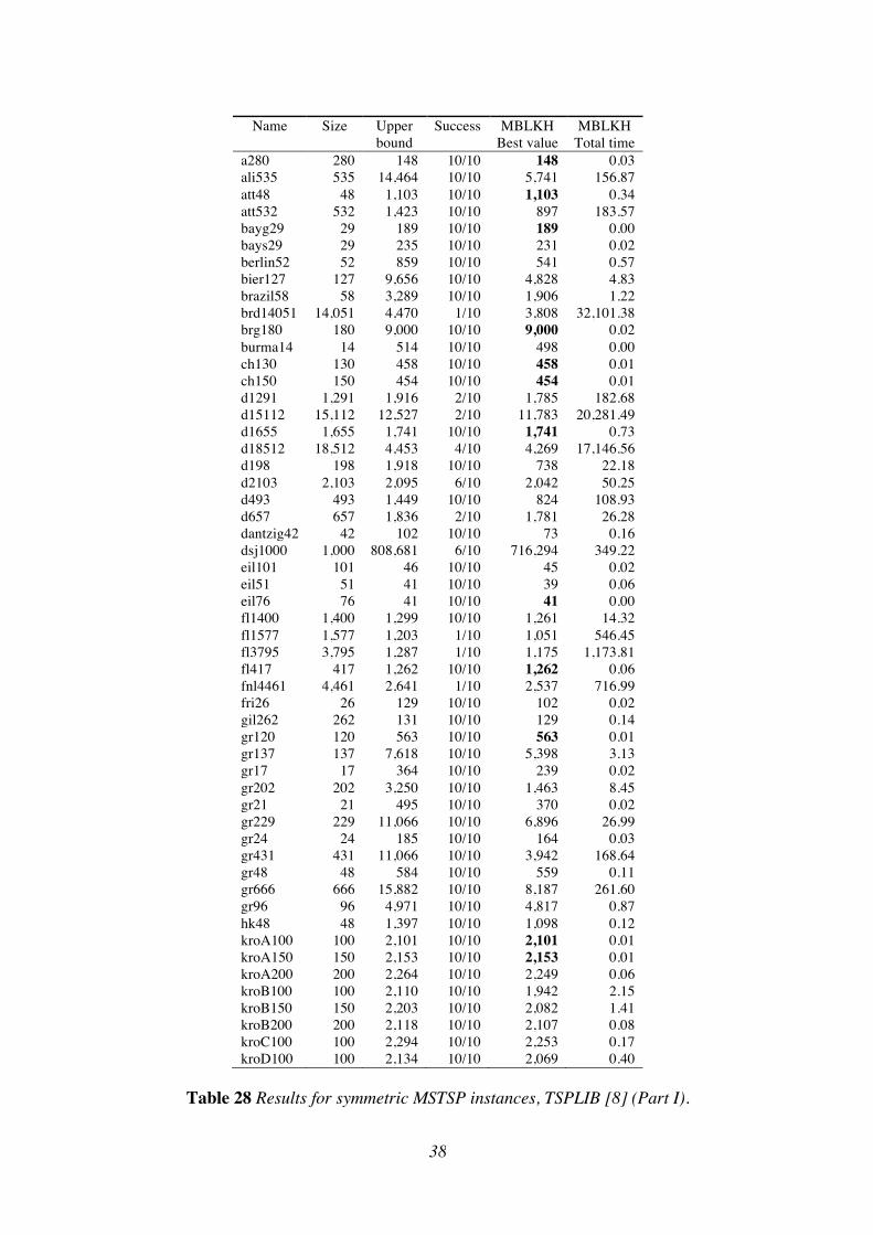
It is well known that the MSTSP on cost matrix cij can be formulated as a BTSP using the transformation c’ij = M - cij, where M is max{cij }. Thus, BLKH can be used for solving the MSTSP after a minor revision. The performance of this revised version, called MBLKH, has been evaluated on the same asymmetric instances as used by John LaRusic et al. [10]. The computational results are com-pared in Tables 26-27. As can be seen, the same best values are found, but MBLKH uses much less CPU time. The performance of MBLKH has also been evaluated on symmetric instances. The computa-tional results for all symmetric TSPLIB instances with up to 18,512 vertices are shown in Ta-bles 28-29. It is to be noted that whereas the asymmetric instances were quickly solved by MBLKH, solution of some of the symmetric instances consume considerably long CPU time, and the best value is found in only 1 out of 10 tests (Success = 1/10). Symmetric MSTSP in-stances are challenging for MBLKH and further research is needed if very large instances of this type are to be solved in a reasonable time.

36

Name Size Upper

bound Success MBLKH

Best value MBLKH

Total time JLR

Best value JLR

Total time coin100.0 100 896 10/10 891 10.81 891 40.99 coin100.1 100 858 10/10 858 0.02 858 14.51 coin100.2 100 974 10/10 974 0.03 974 34.58 coin100.3 100 890 10/10 890 0.01 890 34.12 coin100.4 100 903 10/10 903 0.01 903 10.90 coin316.10 316 1684 10/10 1684 0.11 1684 293.33 crane100.0 100 647,354 10/10 647,354 0.01 647,354 0.30 crane100.1 100 627,751 10/10 627,751 0.01 627,751 0.11 crane100.2 100 645,372 10/10 645,372 0.01 645,372 0.22 crane100.3 100 629,932 10/10 629,932 0.01 629,932 36.57 crane100.4 100 619,054 10/10 619,054 0.01 619,054 0.23 crane316.10 316 664,713 10/10 664,713 0.10 664,713 385.49 disk100.0 100 4,767,083 10/10 4,767,083 0.98 4,767,083 78.04 disk100.1 100 4,882,684 10/10 4,882,684 0.99 4,882,684 31.31 disk100.2 100 4,959,789 10/10 4,959,789 0.01 4,959,789 1.24 disk100.3 100 4,663,663 10/10 4,663,663 0.08 4,663,663 57.06 disk100.4 100 49,971 10/10 4,849,971 0.02 4,849,971 57.94 disk316.10 316 4,947,068 10/10 4,947,068 0.27 4,947,068 416.43 rtilt100.0 100 529,202 10/10 529,202 0.01 529,202 0.24 rtilt100.1 100 546,234 10/10 546,234 0.01 546,234 0.13 rtilt100.2 100 494,714 10/10 494,714 0.01 494,714 0.16 rtilt100.3 100 500,897 10/10 500,897 0.01 500,897 0.13 rtilt100.4 100 517,383 10/10 517,383 0.01 517,383 0.12 rtilt316.1 316 509,367 10/10 509,367 0.13 509,367 1.06 shop100.0 100 1939 10/10 1939 0.01 1939 6.12 shop100.1 100 1786 10/10 1786 0.01 1786 0.10 shop100.2 100 2466 10/10 2466 0.02 2466 57.33 shop100.3 100 2044 10/10 2044 0.01 2044 0.37 shop100.4 100 2104 10/10 2104 0.01 2104 4.07 shop316.10 316 1966 10/10 1966 0.15 1966 1.06 stilt100.0 100 1,011,282 10/10 1,011,282 0.01 1,011,282 0.11 stilt100.1 100 1,071,396 10/10 1,071,396 0.01 1,071,396 0.14 stilt100.2 100 957,076 10/10 957,076 0.01 957,076 0.11 stilt100.3 100 997,468 10/10 997,468 0.01 997,468 0.12 stilt100.4 100 985,154 10/10 985,154 0.01 985,154 0.12 stilt316.10 316 990,472 10/10 990,472 0.12 990,472 0.85 super100.0 100 16 10/10 16 0.01 16 0.09 super100.1 100 16 10/10 16 0.01 16 0.09 super100.2 100 1 10/10 61 0.01 61 0.09 super100.3 100 16 10/10 16 0.01 16 0.09 super100.4 100 16 10/10 16 0.01 16 0.10 super316.10 316 17 10/10 17 0.04 17 0.49 ftv180 181 180 10/10 180 0.05 180 0.34 uk66 66 609 10/10 604 0.47 604 12.52

Table 26 Results for asymmetric MSTSP instances [10] (Part I).

37

Name Size Upper bound

Success MBLKH Best value

MBLKH Total time

JLR Best value

JLR Total time

balas84 84 84 10/10 29 0.01 29 0.06 balas108 108 108 10/10 24 0.01 24 0.09 balas120 120 120 10/10 29 0.01 29 1.04 balas160 160 160 10/10 31 0.02 31 0.18 balas200 200 200 10/10 32 0.03 32 0.23 ran500.0 500 500 10/10 1,000 0.12 1,000 2.06 ran500.1 500 500 10/10 997 0.11 997 1.28 ran500.2 500 500 10/10 997 0.11 997 1.43 ran500.3 500 500 10/10 998 0.11 998 1.92 ran500.4 500 500 10/10 996 0.12 996 1.08 ran1000.0 1,000 1,000 10/10 1,000 0.45 1,000 9.79 ran1000.1 1,000 1,000 10/10 1,005 0.44 1,005 7.55 ran1000.2 1,000 1,000 10/10 1,004 0.44 1,004 5.82 ran1000.3 1,000 1,000 10/10 1,004 0.44 1,004 2.60 ran1000.4 1,000 1,000 10/10 1,006 0.44 1,006 50.92 br17 17 17 10/10 5 0.00 5 0.02 ft53 53 53 10/10 379 0.00 379 0.06 ft70 70 70 10/10 976 0.01 976 9.81 ftv33 34 34 10/10 143 0.00 143 0.02 ftv35 36 36 10/10 154 0.00 154 0.02 ftv38 39 39 10/10 154 0.00 154 0.03 ftv44 45 45 10/10 162 0.00 162 0.03 ftv47 48 48 10/10 168 0.00 168 0.03 ftv55 56 56 10/10 154 0.01 154 0.05 ftv64 65 65 10/10 160 0.01 160 0.05 ftv70 71 71 10/10 161 0.01 161 0.09 ftv90 91 91 10/10 148 0.01 148 22.67 ftv100 101 101 10/10 155 0.01 155 23.17 ftv110 111 111 10/10 165 0.01 165 21.22 ftv120 121 121 10/10 165 0.01 165 0.87 ftv130 131 131 10/10 172 0.02 172 0.17 ftv140 141 141 10/10 172 0.02 172 0.46 ftv150 151 151 10/10 178 0.02 178 0.23 ftv160 161 161 10/10 178 0.02 178 0.19 ftv170 171 171 10/10 180 0.03 180 0.94 kro124p 100 100 10/10 2,347 0.01 2,347 0.15 p43 43 43 10/10 17 0.00 17 2.12 rbg323 323 323 10/10 23 0.11 23 78.19 rbg358 358 358 10/10 21 0.15 21 4.49 rbg403 403 403 10/10 19 0.21 19 43.47 rbg443 443 443 10/10 18 0.27 18 8.90 ry48p 48 48 10/10 1,232 0.01 1,232 11.43

Table 27 Results for asymmetric MSTSP instances [10] (Part II).

38

Name Size Upper bound

Success MBLKH Best value

MBLKH Total time

a280 280 148 10/10 148 0.03 ali535 535 14,464 10/10 5,741 156.87 att48 48 1,103 10/10 1,103 0.34 att532 532 1,423 10/10 897 183.57 bayg29 29 189 10/10 189 0.00 bays29 29 235 10/10 231 0.02 berlin52 52 859 10/10 541 0.57 bier127 127 9,656 10/10 4,828 4.83 brazil58 58 3,289 10/10 1,906 1.22 brd14051 14,051 4,470 1/10 3,808 32,101.38 brg180 180 9,000 10/10 9,000 0.02 burma14 14 514 10/10 498 0.00 ch130 130 458 10/10 458 0.01 ch150 150 454 10/10 454 0.01 d1291 1,291 1,916 2/10 1,785 182.68 d15112 15,112 12,527 2/10 11,783 20,281.49 d1655 1,655 1,741 10/10 1,741 0.73 d18512 18,512 4,453 4/10 4,269 17,146.56 d198 198 1,918 10/10 738 22.18 d2103 2,103 2,095 6/10 2,042 50.25 d493 493 1,449 10/10 824 108.93 d657 657 1,836 2/10 1,781 26.28 dantzig42 42 102 10/10 73 0.16 dsj1000 1,000 808,681 6/10 716,294 349.22 eil101 101 46 10/10 45 0.02 eil51 51 41 10/10 39 0.06 eil76 76 41 10/10 41 0.00 fl1400 1,400 1,299 10/10 1,261 14.32 fl1577 1,577 1,203 1/10 1,051 546.45 fl3795 3,795 1,287 1/10 1,175 1,173.81 fl417 417 1,262 10/10 1,262 0.06 fnl4461 4,461 2,641 1/10 2,537 716.99 fri26 26 129 10/10 102 0.02 gil262 262 131 10/10 129 0.14 gr120 120 563 10/10 563 0.01 gr137 137 7,618 10/10 5,398 3.13 gr17 17 364 10/10 239 0.02 gr202 202 3,250 10/10 1,463 8.45 gr21 21 495 10/10 370 0.02 gr229 229 11,066 10/10 6,896 26.99 gr24 24 185 10/10 164 0.03 gr431 431 11,066 10/10 3,942 168.64 gr48 48 584 10/10 559 0.11 gr666 666 15,882 10/10 8,187 261.60 gr96 96 4,971 10/10 4,817 0.87 hk48 48 1,397 10/10 1,098 0.12 kroA100 100 2,101 10/10 2,101 0.01 kroA150 150 2,153 10/10 2,153 0.01 kroA200 200 2,264 10/10 2,249 0.06 kroB100 100 2,110 10/10 1,942 2.15 kroB150 150 2,203 10/10 2,082 1.41 kroB200 200 2,118 10/10 2,107 0.08 kroC100 100 2,294 10/10 2,253 0.17 kroD100 100 2,134 10/10 2,069 0.40

Table 28 Results for symmetric MSTSP instances, TSPLIB [8] (Part I).

39

Name Size Upper bound

Success MBLKH Best value

MBLKH Total time

kroE100 100 2,165 10/10 2,002 1.61 lin105 105 1,594 10/10 1,477 0.80 lin318 318 2,441 7/10 2,408 3.87 nrw1379 1,379 1,480 10/10 1,382 206.03 p654 654 3,157 10/10 3,157 0.11 pa561 561 94 8/10 84 14.47 pcb1173 1,173 1,656 10/10 1,636 16.41 pcb3038 3,038 2,417 4/10 2,412 90.18 pcb442 442 2,202 10/10 2,202 0.06 pla7397 7,397 491,806 10/10 491,806 33.59 pr1002 1,002 8,917 10/10 8,296 61.97 pr107 107 8,254 10/10 6,826 0.02 pr124 124 7,377 10/10 7,377 0.01 pr136 136 8,237 10/10 8,237 0.01 pr144 144 7,836 10/10 7,224 0.66 pr152 152 8,387 10/10 8,265 0.06 pr226 226 9,510 10/10 9,360 0.58 pr2392 2,392 8,668 10/10 8,668 1.50 pr264 264 6,626 10/10 6,569 4.80 pr299 299 3,480 10/10 3,480 0.04 pr439 439 6,502 10/10 3,909 88.54 pr76 76 11,607 10/10 9,214 0.47 rat195 195 152 10/10 152 0.01 rat575 575 268 10/10 268 0.09 rat783 783 313 10/10 313 0.18 rat99 99 111 10/10 111 0.01 rd100 100 672 10/10 672 0.01 rd400 400 698 10/10 698 0.05 rl11849 11,849 10,970 1/10 10,130 28,339.12 rl1304 1,304 10,690 3/10 9,849 272.61 rl1323 1,323 10,654 2/10 10,289 158.66 rl1889 1,889 10,774 10/10 10,709 11.01 rl5915 5,915 10,661 1/10 10,110 5,793.81 rl5934 5,934 10,776 1/10 9,725 7,874.85 si1032 1,032 429 10/10 429 0.24 si175 175 304 10/10 304 0.01 si535 535 396 9/10 282 28.56 st70 70 63 10/10 63 0.00 swiss42 42 156 10/10 129 0.08 ts225 500 8,485 10/10 8,485 0.02 tsp225 225 262 8/10 233 3.57 u1060 1,060 9,224 10/10 8,345 177.94 u1432 1,432 3,538 10/10 3,500 7.20 u159 159 3,406 10/10 3,406 0.01 u1817 1,817 1,568 10/10 1,557 26.42 u2152 2,152 1,568 10/10 1,563 1.94 u2319 2,319 3,466 10/10 3,421 6.94 u574 574 1,719 10/10 1,568 45.14 u724 724 1,561 10/10 1,561 0.14 ulysses16 16 941 10/10 677 0.03 ulysses22 22 941 10/10 687 0.04 usa13509 13,509 247,403 1/10 171,745 261,458.72 vm1084 1,084 10,337 4/10 10,337 7.05 vm1748 1,748 10,896 10/10 10,896 0.74

Table 29 Results for symmetric MSTSP instances, TSPLIB [8] (Part II).

40

6. Conclusion

This paper has evaluated the performance of LKH on the BTSP and the MSTSP. Extensive tests have shown that the performance is quite impressive. For all BTSP instances either the best known solution were found or improved, and it was possible to find optimum solutions for a series of large-scale instances with up to one million vertices. The developed software is free of charge for academic and non-commercial use and can be downloaded in source code via http://www.ruc.dk/~keld/research/BLKH/.

41

References

1. Vairaktarakis, G. L., On Gilmore-Gomory’s open question for the bottleneck TSP. Oper. Res. Lett. 31:483-491 (2003)

2. Kao, M.-Y. and Sanghi, M., An approximation algorithm for a bottleneck traveling sales-man problem. J. Discrete Algorithms 7:315-326 (2009)

3. Kabadi, S. and Punnen A. P., The Bottleneck TSP. In: Gutin G. and Punnen A. P., editors.

The traveling salesman problem and its variations. Kluwer Academic Publishers, Chapter 15, pp. 489-584 (2002)

4. Edmonds J. and Fulkerson F., Bottleneck extrema. J. Comb. Theory 8:435–48 (1970) 5. Helsgaun, K.: An Effective Implementation of the Lin-Kernighan Traveling Salesman

Heuristic. Eur. J. Oper. Res., 126(1):106-130 (2000) 6. Helsgaun, K.: General k-opt submoves for the Lin-Kernighan TSP heuristic. Math. Prog.

Comput., 1(2-3):119-163 (2009) 7. Lin, S, Kernighan, B.W.: An effective heuristic algorithm for the traveling salesman prob-

lem. Oper. Res., 21(2):498-516 (1973) 8. Reinelt, G.: TSPLIB - a traveling salesman problem library. ORSA J. Comput., 3(4):376-

384 (1991) 9. LaRusic, J., Punnen, A. P., Aubanel, E.: Experimental analysis of heuristics for the bottle-

neck traveling salesman problem. J. Heuristics 18:473-503 (2012) 10. LaRusic, J., Punnen, A. P.: The asymmetric bottleneck traveling salesman problem: Algo-

rithms, complexity and empirical analysis. Comput. Oper. Res. 43:20-35 (2014) 11. Jonker R. and Volgenant T., Transforming asymmetric into symmetric traveling salesman

problems. Oper. Res. Lett. 2:161–163 (1983) 12. Applegate D. L., Bixby R. E., Chvátal V., Cook W.J., Concorde TSP solver.

http://www.math.uwaterloo.ca/tsp/concorde/ (Last updated: October 2005) 13. Johnson, D. S., McGeoch, L. A.: Benchmark Code and Instance Generation Codes.

http://dimacs.rutgers.edu/Challenges/TSP/download.html (Last updated: December 2008) 14. Cook, W.: The traveling salesman problem.

http://www.math.uwaterloo.ca/tsp/index.html (Last updated: September 2013) 15. Fischetti M, Lodi A, Toth P. Exact methods for the asymmetric traveling salesman

problem. In: Gutin G. and Punnen A. P., editors. The traveling salesman problem and its variations. Kluwer Academic Publishers, Chapter 4, pp. 169-205 (2002)

42

16. Held, M, Karp, R.M.: The traveling salesman problem and minimum spanning trees. Oper. Res., 18(6):1138-1162 (1970)

17. Penavic, K.: Optimal firing sequences for CAT scans. Manuscript, Dept. Appl. Math., SUNY, Stony Brook (1994)