Solving the weighted Maximum Constraint Satisfaction Problem using Dynamic and Iterated Local Search Diana Kapsa University of British Columbia Department of Computer Science [email protected]Jacek Kisynski University of British Columbia Department of Computer Science [email protected]Abstract Weighted Max-CSP is one of the NP-hard problems that has been studied for a long time due to its relevance for various research areas e.g. operations research. Nevertheless, stochas- tic local search methods for solving weighted Max-CSP remain largely unexplored. In this project we developed different variants of Iterated and Dynamic Local Search algorithms and empirically analyzed them. The obtained results give a solid basis for a further development of more sophisticated algorithms for weighted Max-CSP. 1 Introduction An instance of the constraint satisfaction problem (CSP) is defined by a set of variables, a domain for each variable and a set of constraints. A solution is a variable assignment for all variables that satisfies all constraints. Max-CSP can be regarded as the generalization of CSP; the solu- tion maximizes the number of satisfied constraints. Max-CSP is usually considered with regards to over-constrained CSP instances, in which it is often impossible to satisfy all constraints. In weighted Max-CSP, each constraint is associated with a positive real value as a weight. The solution maximizes the total sum of the satisfied constraints weights. Weights reflect the impor- tance of constraints. In particular, they might be used to encode distinction between hard and soft constraints. Solving the weighted max-CSP problem is computationally hard, as it is the generalization of the CSP problem, which is NP -complete. An example of a problem that can be naturally encoded into Max-CSP is university examination timetabling ([6]). Another practical example is radio link frequency assignment ([1], [2]). Such problems involve different categories of constraints according to their relevance. 111
Transcript
Solving the weighted Maximum Constraint SatisfactionProblem using Dynamic and Iterated Local Search
Weighted Max-CSP is one of the NP-hard problems that has been studied for a long time dueto its relevance for various research areas e.g. operations research. Nevertheless, stochas-tic local search methods for solving weighted Max-CSP remain largely unexplored. In thisproject we developed different variants of Iterated and Dynamic Local Search algorithms andempirically analyzed them. The obtained results give a solid basis for a further developmentof more sophisticated algorithms for weighted Max-CSP.
1 Introduction
An instance of the constraint satisfaction problem (CSP) is defined by a set of variables, a domainfor each variable and a set of constraints. A solution is a variable assignment for all variablesthat satisfies all constraints.Max-CSP can be regarded as the generalization of CSP; the solu-tion maximizes the number of satisfied constraints. Max-CSP is usually considered with regardsto over-constrained CSP instances, in which it is often impossible to satisfy all constraints. Inweighted Max-CSP, each constraint is associated with a positive real value as a weight. Thesolution maximizes the total sum of the satisfied constraints weights. Weights reflect the impor-tance of constraints. In particular, they might be used to encode distinction between hard and softconstraints.
Solving the weighted max-CSP problem is computationally hard, as it is the generalization of theCSP problem, which isNP-complete.
An example of a problem that can be naturally encoded into Max-CSP isuniversity examinationtimetabling([6]). Another practical example isradio link frequency assignment([1], [2]). Suchproblems involve different categories of constraints according to their relevance.
111
1.1 Formal Definitions
The formal definitions ofCSP instance, weighted CSP instance, variable assignmentandweightedMax-CSP problemare as follows [9]:
Definition 1.1 (CSP instance)A CSP instanceis a triple P = (V,D,C), whereV = {x1, x2,. . . , xn} is a finite set ofn variables,D is a function that maps each variablexi to the setD(xi)of possible values it can take (domain ofxi) and C = {C1, C2, . . . , Cm} is a finite set of con-straints. Each constraintCj is a relation over an ordered setV ar(Cj) of variables fromV, i.e.,for V ar(Cj) = {y1, y2, . . . , yk}, Cj ⊆ D(y1) ×D(y2) × . . . ×D(yk). The elements of the setCj are calledsatisfying tuples ofCj andk is calledthe arity of the constraintCj
In abinary CSP instance, the constraints are unary or binary.
Definition 1.2 (Weighted CSP instance)A weighted CSP instanceis a pair (P,w), whereP isa CSP instance andw : {Cj |j ∈ [1, 2, . . . ,m]} 7→ R
+ is a function that assigns a positive realvalue to each constraintCj of P. w(Cj) is called theweightof constraintCj
Definition 1.3 (Variable assignment)Given the CSP instanceP = (V,D,C), a variable as-signmentof P is a mappinga : V 7→
⋃{D} that assigns to each variablexi ∈ V a value from
its domainD(xi). Assign(P) denotes the set of all possible variable assignments for P.
Definition 1.4 (Weighted Max-CSP) Given a weighted CSP instanceP′ = (P,w), let f(P′,a)be the total weight of constraints ofP satisfied under variable assignmenta :
f(P′,a) =m∑j=1
{w(Cj)|Cj is a constraint ofP anda satisfiesCj}.
The weighted Max-CSPproblem is to find a variable assignmenta∗ that maximizes the totalweight of the satisfied constraints inP :
a∗ ∈ argmin{f(P′,a)|a ∈ Assign(P)}.
Asargmin{f(P′,a)|a ∈ Assign(P)} == argmax{
∑w(Cj)− f(P′,a)|Cj is a constraint ofP ∧ a ∈ Assign(P)} ,
weighted Max-CSP might be considered as a minimization problem, where the objective is to finda variable assignment which minimizes the total weight of the unsatisfied constraints. In our paperwe use the minimization approach.
In the rest of this paper, we focus on the binary weighted Max-CSP with positive integer weights1
andD(x1) = D(x2) = . . . = D(xn) ⊂ N+.1This does not result in the loss of generality, asn-ary relations can be described using binary relations and real
weights can be scaled into integers.
112
2 Related Works
Among the previously applied methods for solving Max-CSP, complete algorithms like branch-and-bound and backtracking based techniques [18] play an important role. Exponential growthof the complexity with growing instance size is their main disadvantage. Besides, for practice re-lated problems like scheduling as well as for large-scale instances, achieving a guaranteed optimalsolution might be extremely time consuming.
As both the best solution quality and the required run time (CPU-time or iterations number) areimportant criteria for measuring the performance of a Max-CSP solver, incomplete techniques getmore interesting. Even though not much work has been done in this area, several stochastic localsearch algorithms have been developed that had a major impact on all later contributions.
2.1 The Min-Conflict-Heuristic
One of the first major efforts for solving the CSP using SLS has been made by Minton et al. [13].Although their algorithm addresses the CSP rather than the Max-CSP, it inspired several of thelater native Max-CSP solvers. As it is often used as a comparison criterion for the performance ofthe different algorithms, we will also consider this algorithm in our experiments.
TheMin-Conflicts heuristicis driven by the idea of ”repairing a complete but inconsistent assign-ment by reducing inconsistencies”. The original version of the algorithm starts with an initialrandom assignmenta : V 7→
⋃{D} and a valuef(a) of the objective function. In each local
search step first a variablexi is chosen uniformly at random from the conflict setC(a). Given theassignmenta, the conflict set is defined as the set of all variablesxi ∈ V that appear in at leastone currently violated constraint (see Figure 1). In a second step a valued ∈ D(xi) is chosen (1-exchange neighborhood) such, that by assigningd to xi the total number of subsequently violatedconstraints is minimized. Among several values that satisfy this criterion, one is chosen uniformlyat random.
Based on this value-ordering heuristic, anIterated Improvementvariant can be applied to theMax-CSP, theMCH . In this case the objective function value is given by sum of weights of allviolated constraints under the assignmenta. After generating an initial random assignment, ineach search step the algorithm tries to minimize the total weight of the violated constraints forthe randomly selected variable. After randomly choosing a variablexi from the current conflictset, MCH computes the sum of the weights of the violated constraints related to this variablexifor all possible domain values. From the best-scored values (there might be several candidateswith equal objective function value) the algorithm then selects one uniformly at random. MCHterminates when the specified solution quality has been achieved or a fixed number of iterationshas been exceeded. The step function implementation is using the neighborhood evaluation tablepresented in 5.3, of complexityO(|D|). The resulting pseudo code is listed in Figure 1.
While efficient in terms of run time, the algorithm has no possibility to escape from a local min-imum and the Min-Conflicts heuristic has a major drawback: stagnation. Based on this, severalother variants have been developed. In their studies on the unweighted Max-CSP, Galinier and
113
procedurebasicMCH(π′)input: problem instanceπ′ ∈ Π′
output: solutions ∈ S(π′) or ∅;s:= init(π′)s:=swhile not terminate(π′, s) dos:= mch step(π′, s)if f(π′, s) ≤ f(π′, s) thens:=s
endendif s ∈ S′(π′) then
return selse
return ∅end
endbasicMCH
proceduremch step(π, s)input: problem instanceπ, candidate solutions;output: candidate solutions′;
C = {xi ∈ V|xi is a variable currently in conflict}xi:= randomfrom set(C)I∗(s, xi) = {d ∈ D(xi)|d minimizes the total weight of currently violated constrains
in whichxi appears}d∗:= randomfrom set(I∗(s, xi))s′:= s|xi=d∗return s′
endmch step
Figure 1: MCH on Max-CSP; init(π′) returns a random candidate solution using a uniform dis-tribution; randomfrom set(A) returns a random element from setA using a uniform distribution;S′(π′) is the set of feasible solutions; a feasible solution is defined as a variable assignment andaccording to the Definition 1.3, depends onV andD.
Hao [8] compared the performance of their Tabu Search variant to that of a Min-Conflict algo-rithm combined with a random-walk strategy, theWMCH [19].
After choosing a conflicting variablexi as already mentioned, the WMCH picks randomly a valued from thexi domain spaceD(xi) with probabilitywp. With probability1−wp, it performs likea basic MCH step. Considering the weight of violated constraints instead of their number, one caneasily extend this algorithm to solve Max-CSP (Figure 2). This basic noise strategy leads to animproved performance, as can be concluded from our experimental results (see Figure 10).
114
procedureWMCH(π′, wp)input: problem instanceπ′ ∈ Π′, walk probabilitywp;output: solutions ∈ S(π′) or ∅;s:= init(π′)s:= swhile not terminate(π′, s) do
with probabilitywp doC = {xi ∈ V|xi is a variable currently in conflict}xi:= randomfrom set(C)d:= randomfrom set(D(xi))s:= s|xi=d
otherwises:= mch step(π′, s)
endif f(π′, s) ≤ f(π, s) thens:=s
endendif s ∈ S′(π′) then
return selse
return ∅end
endWMCH
Figure 2: WMCH on Max-CSP; init(π′) returns random candidate solution using uniform distribu-tion; randomfrom set(A) returns random element from setA using uniform distribution;S′(π′)is the set of feasible solutions.
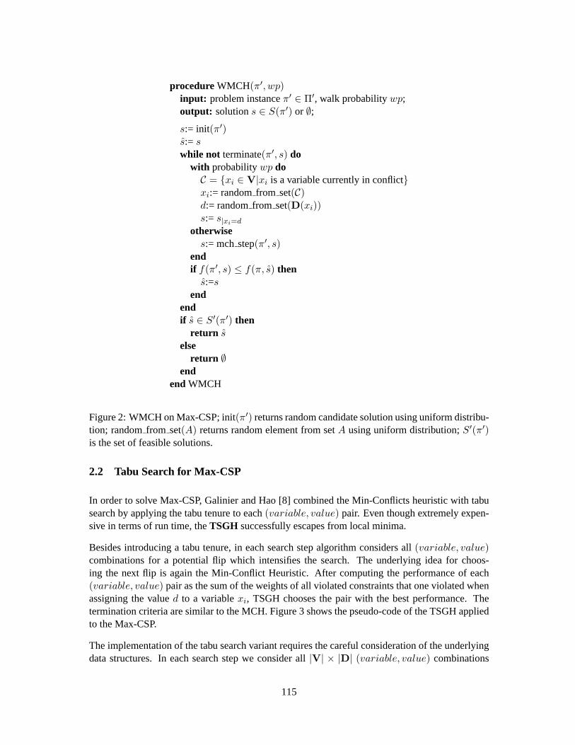
2.2 Tabu Search for Max-CSP
In order to solve Max-CSP, Galinier and Hao [8] combined the Min-Conflicts heuristic with tabusearch by applying the tabu tenure to each(variable, value) pair. Even though extremely expen-sive in terms of run time, theTSGH successfully escapes from local minima.
Besides introducing a tabu tenure, in each search step algorithm considers all(variable, value)combinations for a potential flip which intensifies the search. The underlying idea for choos-ing the next flip is again the Min-Conflict Heuristic. After computing the performance of each(variable, value) pair as the sum of the weights of all violated constraints that one violated whenassigning the valued to a variablexi, TSGH chooses the pair with the best performance. Thetermination criteria are similar to the MCH. Figure 3 shows the pseudo-code of the TSGH appliedto the Max-CSP.
The implementation of the tabu search variant requires the careful consideration of the underlyingdata structures. In each search step we consider all|V| × |D| (variable, value) combinations
115
procedureTSGH(π′, f, tl)input: problem instanceπ′ ∈ Π′, objective functionf(Π′), tabu tenuretl;output: solutions ∈ S(π′) or ∅;s:= init(π′)init tabu list(tl)s:=swhile not terminate(π′, s) doI(s) = {(xi, d), xi ∈ V, d ∈ D(xi)|(xi, d) not tabu orf(π′, s|xi=d) ≤ f(π′, s)}I∗(s) = {(xi, d) ∈ I(s)| assigningd to xi minimizes the total weight of conflicts forxi}(x∗i , d
Figure 3: TSGH on Max-CSP; init(π′) returns candidate solution chosen randomly using a uni-form distribution; init tabu list(tl) randomly initializes the tabu list using a uniform distribution;randomfrom set(A) returns a random element from setA using a uniform distribution;updatetabu list((xi, d), tl) adds the pair(xi, d) to the tabu list and removes the oldest pair if thelength of the tabu list is greater thantl; S′(π′) is a set of feasible solutions.
instead of allk possible values for one randomly chosen variable. As already mentioned thecomputation of the evaluation function value for each of the|V|× |D| pairs requires timeO(|D|).Consequently, the implementation of the step function of the TSGH has time complexityO(|V|×|D|).
Since the choice of the next step is much greedier, we expect a better performance in terms ofsolution quality, but a worse performance in terms of run time. In order to compensate for thehigher complexity of each search step, we can use special data structures to find the neighbor withthe best evaluation function in the current neighborhood (see Section 5).
Figure 10 compares the performance of all algorithms on randomly generated instances from theUniform Binary Random Model (see section 6.1) from the same instance classes as used by Galin-ier and Hao [8], but additionally using constraint weights, each random uniformly chosen from adomain[0, . . . , 99].
In Section 5 we present major implementation issues more in detail, as well as their impact on the
116
performance of the so far described algorithms and on the instance size used for the experimentalwork.
2.3 Randomized Rounding with MCH
The latest major contribution by Lau [11] combines a new approximation method based on ran-domized rounding and semidefinite programming with the already described MCH. His experi-mental results show this new algorithm to perform better than both the MCH and WMCH on solv-able, random instances. Unfortunately, he does not compare the performance of his new algorithmto that of the TSGH. The satisfiable randomly generated instances used by Lau are also availablein an unweighted version on the web site of van Beek [4], whose main research concentrates onsolving binary CSPs using backtracking methods.
3 Iterated Local Search
As one of the rather straight-forward but powerful SLS methods,ILS (Iterated Local Search) triesto achieve a good tradeoff between intensification via local search methods and diversification byusing a perturbation procedure after each encountered local minimum. As a further important ele-ment of this framework, an acceptance criterion is used to control the balance between perturbationand local search.
Clearly the ILS depends highly on the quality of the underlying stochastic local search procedure.The greedier this procedure is, the more effective the perturbation is required to be. The com-bination of the already mentioned key elements of an Iterated Local Search algorithm is ideallychosen in such a way that the results achieved are better than just sequentially performing severalstochastic local search steps.
Based on the mentioned in Section 2 local search strategies we considered several variants ofILS: ILS-MCH , ILS-WMCH and ILS-TSGH . Due to the different run-time performance andachieved solution quality it is not obvious that the greediest local search strategy, TSGH, wouldlead to better results in this more general framework.
For perturbation we choose between different approaches. Besides random picking, we can use afixed number of random walk steps. Using a random noise strategy shows considerable improve-ment in the case of the WMCH. Consequently, a perturbation procedure based on a fixed numberof random walk steps should likewise help escaping from local minima. We also considered athird perturbation strategy - a random flip of a non-conflicting variable - but tests showed that itdid not improve solution quality.
We denote algorithms with random picking as perturbation with the suffix “-RP”, those with ran-dom walk steps with the suffix “-RS”.
The acceptance criterion compares the current solution to that one of the previous iteration andchooses the better with respect to the objective functionf(π, s) with a certain acceptance proba-
117
procedure ILS-WMCH(π′, wp, bp, ws)input: problem instanceπ′ ∈ Π′, objective functionf(Π′), walk probabilitywp,
acceptance probabilitybp, number of random walk stepsws;output: solutions ∈ S(π′) or ∅;s:= init(π′)s:= ls-WMCH(π′, f, wp, s)s:= swhile not terminate(π′, s) dos′:= perturb(π′, s, n)s′′:= ls-WMCH(π′, s′)if f(π′, s′′) ≤ f(π, s) thens:=s′′
ends:= accept(π′, s, s′′, bp)
endif s ∈ S′(π′) then
return selse
return ∅end
end ILS-WMCH
Figure 4: ILS-WMCH on Max-CSP; init(π′) returns a random candidate solution using a uniformdistribution; ls-WMCH is equivalent to WMCH presented in Figure 2, except it does not have theinitialization procedure;S′(π′) is a set of feasible solutions.
bility bp. The higher the acceptance probability the greedier the algorithm, and the more likely isthat we will return to the local minimum encountered during the previous iteration. In this case astronger perturbation is required, e.g. a higher number of random walk steps.
The additional complexity due to the ILS framework combined with the distinct stagnation be-havior of the subsidiary local search procedures, except TSGH, motivated an appropriate controlmechanism. When the evaluation function value does not change over a fixed number of itera-tions, the underlying local search is terminated. This fixed number is subject to carefully tuningand varies considerably among the different algorithms. A more detailed description of the tuningprocess is given in 7.1.1.
For each of the developed ILS variants the stagnation control mechanism was motivated as follows:
ILS-MCH: Stagnation is the main drawback of the basic MCH. By including MCH into the ILSscheme we expect to diminish this problem. Using appropriate perturbation and acceptancestrategies, we try to escape from the local optimum achieved in the local search procedure.Even a very naive perturbation (e.g. random picking) combined with a greedy acceptanceprocedure will surely achieve a better solution quality than the initial MCH.
On the other side this approach increases time complexity fromO(|V| × |D|) for the basic
118
MCH to O(max ils iterations × |V| × |D|), where maxils iterations is the maximumnumber of performed ILS iterations. Consequently, we expect a considerable longer run-time and worse performance in comparison to other non-ILS approaches (e.g. setting themax ils iterations to|V| × |D| leads to the same complexity in case of TSGH).
ILS-WMCH: Although less greedy than the TSGH, WMCH is, due to it’s lower complexity,better with respect to the run-time. The resulting algorithm is presented in Figure 4.
ILS-TSGH: Based on the already presented perturbation and acceptance procedures and in com-bination with a TSGH as local search method, we developed the ILS-TSGH. The interestingquestion arising in this context is about the efficiency of ILS-TSGH compared to that oneof the ILS-WMCH. TSGH considers in each move the entire1-exchange-neighborhood andtries to find the move that leads to the best performance, meaning to minimize the weightof violated constraints for the respective variable. WMCH considers only1
|V| of this neigh-borhood. An appropriate choice of perturbation and acceptance methods could compensatefor the additional quality achieved by the TSGH. As in case of the TSGH, by keeping themaximum number of performed ILS iterations (maxils iterations) below|V|× |D|, we ex-pect especially in case of very large instances to have a comparably good performance. Forthe TSGH, experimental work is required in order to conclude on the gain of using the ILSframework.
4 Dynamic Local Search
Applying Dynamic Local Search (DLS) to more prominent NP-hard problems (particularly toSAT) leads to algorithms that outperform other approaches. Based on this - and additionally moti-vated by the similarities between MAX-SAT and MAX-CSP - we implemented a DLS algorithmfor weighted MAX-CSP.
Unlike all other approaches presented so far, DLS uses a dynamic adjustment of the evaluationfunction in order to escape from local minima. When the subsidiary local search procedure en-counters an optimum, the algorithms changes the evaluation of the found solution such that furtherimprovement can be done. Penalizing the affected solution components is one common way ofimplementing this.
Our DLS algorithm is based on the random walk variant of the min-conflicts based iterative im-provement, WMCH (see Section 2.1), as subsidiary local search procedure. Using the1-exchange-neighborhood, the WMCH is a local conflict driven best improvement algorithm; each move ischosen in a two-step decision process that has onlyO(|D|) complexity compared to the usualO(|V|× |D|) required for scanning the entire neighborhood. The best DLS for SAT uses the stan-dard best improvement technique as underlying local search strategy. However, in case of MAX-CSP, the size of the neighborhood can be considerably larger, due to the nature of the problem.Therefore, a complete scan of the neighborhood is less likely to bring significant improvement.
When penalizing the encountered local minimum, we have to consider the interaction with theoriginal weights associated with each of the constraints. Therefore we choose to penalize each
119
procedureDLS-WMCH-PP(π′)input: problem instanceπ′ ∈ Π′;output: solutions ∈ S(π′) or ∅;s:= init(π′)s:=sinit penalties(π′)while not terminate(π′, s) dog′ = g +
procedureupdatepenalties(π, s)input: problem instanceπ′, candidate solutions;output: penalties tablepenalties;
C = {xi ∈ V|xi is a variable currently in conflict}for eachxi ∈ C dopenalties[i][s[i]]:= penalties[i][s[i]] + p
endreturn penalties
endMCH step
Figure 5: DLS-WMCH-PP on Max-CSP; init(π′) returns a random candidate solution using auniform distribution;penalties is a |V| × |D| matrix in which each element(i, j) indicates thepenalty for considering(xi, dj) as a solution component;penaltiesmatrix is initialized with zerosby procedure initpenalties(π′); g′ guides the local search of the underlying WMCH based localsearch procedure.S is then-dimensional solution matrixS′(π′) is a set of feasible solutions.
solution component, in our case each (variable, value) pair of the solution and derive the followingevaluation function:
g′(π′, s) =∑
(w(Cj)|Cj is an unsatisfied constraint for s)+∑(penalties(xi, dj)|(xi, dj) is a solution component)
Penalizing each(variable, value) pair leads to a similar effect as using a tabu tenure (see Section
120
5.2) but has three major differences:
• Reduced complexity when choosing the next flip compared to TSGH
• Using incremental penalties instead of a fixed tabu tenure leads to algorithms that avoid acertain solution component but not forbid it for a fixed number of iterations.
• The tabu status of a(variable, value) pair is reset after a fixed number of iterations, whilethe penalties, even in the case of smoothing, tend to remain or even increase.
Initially all weights are set to0 as we assume that randomly generated assignment is not a localoptimum. The algorithm penalizes (after each local search phase) the encountered solution byincrementing the respective components by a constant penalty factor. Due to the fact that WMCHhas no special escape mechanism, and due to the increased number of total iterations (inner andouter loop), we use - as in case of the ILS - a stagnation based termination (see Section 3). Theresulting pseudo-code is presented in the Figure 5.
Depending on which of the solution components are penalized at the end of the local search phasewe distinguished, implemented and experimented the three following different variants:
DLS-WMCH-TP: The total penalization variant increases weights for all(variable, value) pairsinvolved in the currently encountered local optimum. The idea is to simply change theevaluation function in such a way that it avoids already analyzed positions in the searchspace.
DLS-WMCH-PP: Here the penalization is restricted to(variable, value) pairs that involve vari-ables from the current conflict set. The motivation behind this variant is to keep good solu-tion components and avoid the rest.
DLS-WMCH-NP: The non-conflicting penalization variant increases weights only of those vari-ables that are currently not violating any constraints. The resulting moves might lead newsolutions that could not be encountered else due to the accepted deterioration of the evalua-tion function.
5 Implementation
In the following we describe interesting implementation aspects that we encountered during theproject.
5.1 Data Structures
During our project, we used a data structure that allows the representation of sufficiently largeunary and binary instances. In a|V| × |V|matrix, whereV is the set of variables, we consider allpossible unary and binary constraints. Each of the elements of this matrix consists of a|D| × |D|
121
matrix, whereD is domain of variables. The|D| × |D| matrix at position(i, j) in the |V| × |V|matrix encodes one constraint between two variablesxi andxj . Position(a, b) in the constraintmatrix at position(i, j) specifies the penalty for assigning the valuesda anddb to xi respectivelyxj . If the value of the element(da, db) is different from0, a constraint is broken when the men-tioned assignment occurs. The element(da, db) corresponds to the weight of this constraint. If thevalue of(da, db) is equal to0, no constraint is broken or its weight is0. For representing largeproblem instances, it turned out to be extremely important to only allocate memory for existingand not for all possible constraints, since the|V| × |V|matrix tends to be sparse.
5.2 Tabu List Implementation
For the implementation of the tabu list we considered two data structures: a linked list of thetabu set elements and a|V| × |D| array for the tabu status of each of the(variable, value) pairs.Whereas the notion of tabu list suggests rather the first alternative, the latter one is the moreefficient option. The time needed for retrieving an element out of a list is linear in the length of thelist, which corresponds to the tabu tenuretl. Therefore, it is comparatively expensive to find outif an element is set tabu. The larger the instance, the higher the optimal tabu tenure is likely to beand consequently the retrieval time. As opposed to this, retrieval from an array requires constanttime. Given the fact that time performance in this context is more important than used memory,we decided in favor of the second alternative.
5.3 Neighborhood Evaluation
Especially in the case of the TSGH, in which we consider the entire1-exchange-neighborhood ineach local search step, the implementation of the neighborhood evaluation is an important issue.Based on the technique described in [8] we used a|V| × |D| array for storing the evaluationfunction values for each move. The element(i, j) in the |V| × |D| matrix specifies the resultingweight of violated conflicts for variablexi that occur when assigning the valuedj to the variablexi. After the random initialization at the beginning of the local search procedure, we compute allmatrix values. Hence we only have to update the|V| affected values in the|V| × |D|matrix aftereach move. Consequently the complexity of each move isO(|V|).
5.4 Random Number Generation
As for every stochastic local search the random number generator is extremely important. Inour case we use a linear congruential generator implementation provided by AT&T (urand.c).The random number generator is initialized by using the current calendar time (function timettime(time t *tp) from the time.h C library). Alternatively the user can specify a random seed forinitialization in order to make results deterministic.
122
6 Instances
6.1 Random Instances - Uniform Random Binary CSP Model
In order to measure and compare the performance of our algorithms to both complete and in-complete approaches, we conducted experiments on randomly generated binary instances. Ourinstances are currently generated according to theUniform Random Binary CSP model([16]).Each instance is characterized by the number of variablesn, the domain sized as well as the den-sity p and the tightnessq of constraints. The densityp describes the probability of a constraintoccurring between two CSP variables, whileq specifies the conditional probability that a valuepair is allowed given that there is a constraint between the two variables.
The higherp and lowerq is, the less likely the instance is to be satisfiable. In the rest of our paperwe call such instances hard. The lowerp and higherq is, the more likely the instance is to besatisfiable. In the rest of our paper we call such instances easy. In our experiments we generatedinstances from the same classes as used by Galinier and Hao [8] up to a number of100 variablesand15 values in each of the respective domains. As also used by [11], we generated instanceswith 20 variables in order to make performance results more comparable. Values forp andq werechosen so that we cover both easier and harder instances. For our tests we used eighteen test-sets,with ten instances in each test-set.
For all instances generated based on the Uniformed Random Binary CSP model we use one weightfor all constraints between each two variables. Full profit of our data structure as described insubsection 5.1 is only taken by the crafted data. Constraint weights are generated uniformly atrandom in a range from[0, . . . , 99].
6.2 Crafted Instances
We planned to use instances of the International Timetabling Competition [12]. The data consistsof 20 instances defining scheduling problems with up to440 events in10− 11 rooms and45 timeslots (5 days,9 hours each day). Additional constraints (hard and soft with different weights)are motivated by feature characterization of events and rooms (up to10 different features in oneinstance), room sizes and student preferences (up to350 students). All instances have a perfectsolution with no broken constraints.
After in-depth analysis of the problem of encoding such instances into weighted Max-CSP in-stances, we decided not to use this data. The reason for this is that timetabling instances involvea lot of k-ary constraints fork > 2. Such constraints might be encoded as multiple binary con-straints (as we only consider unary and binary constraints), but this is fairly difficult, results ingrowth of number of constraints, requires vast amount of memory space for data structures (orrequires functional encoding of constraints) and makes the description of the problem not natural.
123
Figure 6: Network structure of the Philadelphia problems (left); demandD1 (right) (source: [7]).
6.3 Real World Instances
We considered using eithersports tournament schedulinginstances (e.g. in [20]) orfrequencyassignment problem(FAP) instances. We decided to use the latter ones, as different formulationsof the FAP problem are conceptually easier, and instances as well as experiment results are widelyavailable ([7], [5], [15]).
6.3.1 Frequency Assignment Problem
The frequency assignment problem (sometimes also called channel assignment problem) arises inthe area of wireless communication (e.g. GSM networks). One can find many different models ofthe FAP problem (due to many different applications), but they all have two common properties:
i frequencies must be assigned to a set of wireless connections so that communication ispossible for each connection
ii interference between two frequencies (and what follows, quality loss of signal) might occurin some circumstances which depend on:
(a) how close the frequencies are on the electromagnetic band
(b) how close connections are to each other geographically.
There are also many objectives, which define the quality of an assignment - the goal is to obtainthe highest possible quality. Survey [2] gives an extensive overview on different models, prob-lem classifications, applied methods and results. We decided to use the so calledPhiladelphiainstances, which are one of the most widely studied so far in the FAP area.
6.3.2 Philadelphia Instances
Philadelphia instances were introduced in paper [3] in 1973. They describe a cellural phone net-work around Philadelphia (Figure 6, left). The cells of a network are modeled as hexagons2,
2Nowadays this simplified approach is no longer used. Nevertheless, Philadelphia instances are still being explored- the most recent results are available at [7].
each cell requires some number of frequencies (Figure 6, right). Tuples(cell number, number offrequencies required) form ademand vector. Considered demand vectors include:
The distance between different cell centers is1. Frequencies are denoted as positive integer num-bers. Interference of the cells is characterized by a reuse distance vector(d0, d1, d2, d3, d4, d5): dkdenotes the smallest distance between centers of two cells, which can use frequencies that differ byat leastk without interference. Figure 7 shows graphical representation of reuse distance vectorsR1 = (
√12,√
3, 1, 1, 1, 0), R2 = (√
7,√
3, 1, 1, 1, 0) andR3 = (√
12, 2, 1, 1, 1, 0).
The objective is to find frequency assignments which result in no interference and minimize thespan of frequencies used, i.e., the difference between maximum and minimum frequency used.
Figure 8 defines the Philadelphia instances explored in the literature (namedP1-P9 in conformitywith [17]) and provides the value of the optimal solution (minimal span). The instanceP1 is theoriginal instance motivated by the above mentioned cellural phone network.
125
6.3.3 Encoding into Weighted Max-CSP
We encoded Philadelphia instances into the weighted Max-CSP problem structure in the followingway:
variables: each frequency requirement is represented as a single variable, e.g. for demand vectorD1 there are 481 variables,8 of them correspond to the demand of cell1, 25 correspond tothe demand of cell2, etc.
domains: each variable has the same integer domain[0, 1, . . . , l+ d1×WORSTOPTe], wherelis the minimal upper bound known for the particular instance3 and WORSTOPT≥ 1.0 is areal constant.
constraints: constraints are divided into two groups:
hard binary constraints: correspond to the requiment of no occuring interference. A hardconstraint between two locations is set based on the network structure and the reusedistance vector for particular instances. Weights of hard constraints are equal to someinteger number greater than the maximum sum of the weights of the broken soft con-straints.
soft unary constraints: correspond to the minimization of the used frequencies span. Eachpossible variable value is “penalized” by a unary soft constraint with weight:value×FORCEMIN, where FORCEMIN ≥ 1.0 is a real constant andvalue is avalue of the variable.
Setting value of two constants WORSTOPT and FORCEMIN involves following tradeoffs:
• the larger WORSTOPT (which implies bigger domain size), the easier the algorithm maysatisfy hard constraints, but also the bigger the search space will be,
• the larger FORCEMIN (which implies larger weights for soft constraints) the more likelythe algorithm minimizes span, but the more is the algorithm attracted to the smallest fre-quency values (which might occur to be the main weakness of such encoding).
Storing such weighted Max-CSP instances in data structures described in Section 5.1 is not real-istic as it would require approximately12GB − 24TB of memory. Functional encoding of con-straints would result in loss of efficiency. A solution of this problem is based on the observation,that in each instance there are only five types of binary hard constraints (xi − xj ≥ 1, xi − xj ≥2, . . . , xi − xj ≥ 5) and (size of domain) different types of the unary soft constraints.
Constraints are stored in six two-dimensional arrays (five for each hard constraint and one for allsoft constraints), indexed with domain values. Numbers in the arrays describe the total sum ofweights of broken constraints for particular value assignment (0 - no constraint broken). Finally, atwo-dimensional array - which is indexed with variable names - contains for each(vari, varj) pair
3For Philadelphia instances, the best lower bound known is actually the optimal solution, but one may start with6×number of variablesas an obvious upper bound and change it later using results from performed experiments.
126
REPETITIONS of LS STAGNATION FRACTIONAlgorithm Number of variables Number of variables
Figure 9: Local search repetitions and stagnation parameter settings for random instances.
a pointer to one of the six arrays, or a NULL pointer if there is no constraint between the variables.Particularly, for all pairs(vari, vari) a pointer points to the array storing the soft constraints. Allarrays are allocated dynamically, which gives freedom in changing the WORSTOPT parameter.
7 Experiments
All experiments were performed using the LSF load distribution system running on Linux ma-chines. Tuning tests were run on dual 1GHz Intel Pentium III, 256KB cache, 4GB/2GB RAMcomputers, final tests were run on dual 2GHz Intel Xeon, 512KB cache 4GB/2GB RAM comput-ers. The algorithms were implemented in C and compiled with gcc 2.92.2.
7.1 Random Instances
As the instance generator does not guarantee that instances satisfiable and because of the size ofthe instances (exhaustive search would be intractible) we use theabsolute ratio(sum of weightsof satisfied constraints divided by sum of weights of all constraints) to measure and compare theachieved solution quality. In the following, we use the absolute ratio as indicator for the solutionquality. All tuning tests (except stagnation tuning) were quality driven, and time was taken intoaccount if a decision was not possible based on quality performance.
7.1.1 Testing Protocol
All algorithms were tested according to the following rules:
• The number of iterations for MCH, WMCH and TSGH was set to10, 000.
• The number of repetitions of ILS and DLS local search and the stagnation limit (determiningtermination - see section 3) of ILS and DLS local search were determined through some pre-tuning tests (in case of ILS with random picking as perturbation and probability of accepting
127
a better solution set to1.0, in case of DLS with penaltyp set to1). The stagnation limit wastuned in order to obtain the highestmoves/iterations ratio and minimum iterations num-ber without significant loss of solution quality. The number of repetitions was tuned toachieve an overall number of iterations of local search of approximately10, 000 − 20, 000(but no less repetitions then10). Number of iterations of local search had cut-off10000(providing the stagnation criterion did not make it terminate earlier) in order to ensure rea-sonable experiments time. Figure 9 shows the final setting of the parameters.
The stagnation limit showed to be fairly difficult to tune. We found out that some reactivemechanism changing this parameter during search progress might be a better solution.
• ILS and DLS local search algorithms were tuned due to the results obained while testingthem as stand-alone procedures.
• Parameters tuning: consisted of two stages:
Range estimating: 10 runs were performed on each instance in each test-set in order tobound range of parameter values. For each instance and each parameter value, themean absolute ratio was calculated, and then for each test-set the mean over meanabsolute ratios for test-set members was calculated and used to compare performance.
Parameters setting: Based on the results from the previous point, up to10 different pa-rameter values were chosen and test runs performed (10 runs on each instance). Aspreviously, mean over mean absolute ratios for the test-set members was used to de-termine the optimal parameter setting for each test-set of instancess.
• Experiments: Using an optimal parameter setting for each test-set of instances obtainedduring tuning (optimal in sense of obtained solution quality), two kinds of tests were per-formed:
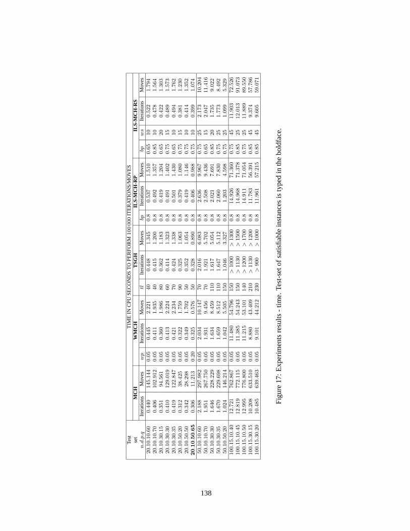
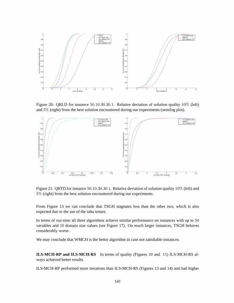
General: 100 runs were performed on each instance in each test-set. For each instance werecalculated: the mean absolute ratio, minimum and maximum absolute ratio, the meannumber of iterations, the mean number of moves (iterations in which some variablewas flipped, it does not include random steps in WMCH and perturbation steps in ILS),the mean moves per iterations fraction, the mean time to perform100, 000 iterations,and the mean time to perform100, 000 moves. Then for each test-set were calculated:the mean over mean absolute ratios for test-set members, minimum and maximummean absolute ratios (Figures 10, 11, and 12), the mean over mean iterations, overmean moves, over mean moves per iterations fraction (Figures 13, 14, 14 and 16),the mean over mean time to perform100, 000 iterations, and over the mean time toperform100, 000 moves (Figures 17, 18 and 19).
Specific: 1000 runs were performed on one instance from each test-set. The obtained datawas used to produce plots.
• ILS and DLS local search algorithms were tuned due to the results obained while testingthem as stand-alone procedures.
128
7.1.2 Tuning
WMCH: Tests with walk probabilitywp set to0.00, 0.20, 0.40, 0.60, 0.80 suggested a rangeof [0.00, 0.40]. Additional tests withwp set to0.05, 0.10, 0.15, 0.20, 0.25, 0.30, 0.35were performed. The value0.05 resulted in the best performance for all test-sets except20.10.50.65. Interestingly,0.20 was the second best value for many instances, and thebest value for instances in the test-set20.10.50.65 (which happend to consist of solvableinstances). Most likely, more detailed tests would result in settingwp to a value smallerthen0.05 for many test-sets.
TSGH: Tests with tabu lengthtl set to0, 50, 100, 150, 200 (except test-sets with20 variables - itwould put all possible(variable, value) pairs on the tabu tenure) suggested range[30, 150]for 20 variables,[70, 200] for 50 variables and[140, 230] for 100 variables. Additional testswith tl changing by10 in every range for corresponding test-sets of instances were done.
For test-sets with20 variables, values between40 and100 resulted in the best performancefor all test-sets. Interestingly, fortl equal to150, mean differed from one for optimal settingon the3rd decimal place while testing test-sets with20 variables and size of domain10. Thissuggests, that implementation of the algorithm which uses techniques prefering stronglyleast recently flipped variables might be worth considering.
For test-sets with50 variables, values between70 and150 variables resulted in the bestperformance. For100 variablestl set to140, 150 for test-sets consisting of easy instancesand set to210, 230 for test-sets consisting of hard instances was optimal.
Very long running time for test-sets with100 variables, did not allow us to test ILS algo-rithms with TSGH as local search on those test-stes.
All tests for TSGH showed that, the harder the instance test-sets as well as the higher thenumber of variables, the longer the tabu tenure is needed in order to achieve optimal perfor-mance.
ILS-MCH-RP: Tests with probability of accepting the best so far solutionbp set to0.25, 0.5 and0.75 suggested no change in solution quality for different values ofbp. Additional tests withbp set to0.1, 0.2, 0.35, 0.45, 0.5, 0.65 and0.8 confirmed this observation. It is quite natural,that the tests had rather debugging motivation, as using random picking as the perturbationmethod renders the acceptance criterion irrelevant. The value0.8 was chosen arbitrarily (astime also did not vary).
ILS-MCH-RS: Tests with probability of accepting the best so far solutionbp set to0.25, 0.5 and0.75 and number of random walk stepsws set to10, 20 and50 (all possible combinations ofthose two parameters) showed thatbp equal to0.75 is the best among three tested settings.The number of random stepsws set to half of the number of variables usually resulted inthe best performance.
Additional tests withbp set to0.65, 0.75, 0.85 andws set to the previously obtained op-timal value for a particular test-set, to value5 larger and to value5 smaller (all possiblecombinations ofbp andws) were run to determine the parameters with a higher precision.
ILS-WMCH-RP: Tests with probability of accepting the best so far solutionbp set to0.25, 0.5and0.75 suggested no change in solution quality for different values ofbp. Additional tests
129
with bp set to0.15, 0.35, 0.45, 0.55, 0.65, 0.7 and0.8 confirmed this observation. Again thetests had rather debugging motivation. The value0.8 was chosen arbitrarily (as time alsodid not vary).
ILS-WMCH-RS: Tests with probability of accepting the best so far solutionbp set to0.25, 0.5and0.75 and number of random walk stepsws set to10, 20 and50 (all possible combina-tions ofbp andws) showed thatbp equal to0.75 is the best among three tested settings. Thenumber of random stepsws equal to10 and20 usually resulted in the best performance.
Additional tests withbp set0.65, 0.75, 0.85 andws set to the previously obtained optimalvalue for a particular test-set, to value5 larger and to value5 smaller (all possible combina-tions ofbp andws) were run to determine the parameters with a higher precision.
ILS-TSGH-RP: Tests with probability of accepting the best so far solutionbp set to0.25, 0.5 and0.75 suggested no change in solution quality for different values ofbp. Additional tests withbp set to0.15, 0.35, 0.45, 0.55, 0.65, 0.7 and0.8 confirmed this observation. Again the testshad rather debugging motivation. The value0.8 was chosen arbitrarily (as time also did notvary).
ILS-TSGH-RS: Tests with probability of accepting the best so far solutionbp set to0.25, 0.5 and0.75 and number of random walk stepsws set to10, 20 and50 (all possible combinationsof those two parameters) showed thatbp equal to0.75 is the usually best among three testedsettings. The number of random stepsws set to10 usually resulted in the best performance.
Additional tests withbp set to previously obtained optimal value for particular test-set, tovalue0.1 larger and to value0.1 smaller andws set to previously obtained optimal value fora particular test-set, to value5 larger and to value5 smaller (all possible combinations ofbpandws) were run to determine the parameters with a higher precision.
DLS-WMCH-TP: Tests with penaltyp set to1, 5 and10 were performed.p setting1 resulted inthe best performance. Additional tests withp set to2, 3 and4 showed that values1 and2are optimal settings for all test-sets.
DLS-WMCH-PP: Tests with penaltyp set to1, 5 and10 were performed.p setting1 resulted inthe best performance. Additional tests withp set to2, 3 and4 showed that values1 and2(in case of test-set100.15.10.50 - 4) are optimal settings for all test-sets.
DLS-WMCH-NP: Tests with penaltyp set to1, 5 and10 were performed. They showed greatvariety in optimal settings. Additional tests withp set to2, 3, 4, 6, 7, 8, 9, 11 and 12confirmed this observation. Values1, 2, 3, 5, 68, 10 and11 resulted in optimal performancefor different test-sets.
7.1.3 Results
MCH, WMCH and TSGH Based on the absolute ratios (Figure 10) we can conclude thatamong the three algorithms WMCH achieves on the average the higher absolute ratios and there-fore the best quality for the same number of iterations. On solvable instances, TSGH alwayssucceeds to solve the instance, but for100 variables it performs significantly worse in terms ofsolution quality than WMCH and even sometimes than MCH.
130
Test
AB
SO
LUT
ER
ATIO
Sse
tM
CH
WM
CH
TS
GH
ILS
-MC
H-R
Pn.d.p.q
Min
Mea
nM
axwp
Min
Mea
nM
axtl
Min
Mea
nM
axbp
Min
Mea
nM
ax20.1
0.1
0.6
00.8
79
0.8
86
0.8
92
0.0
50.9
16
0.9
26
0.9
35
40
0.9
14
0.9
23
0.9
29
0.8
00.9
04
0.9
13
0.9
17
20.1
0.1
0.7
00.9
47
0.9
51
0.9
56
0.0
50.9
73
0.9
79
0.9
87
40
0.9
70
0.9
77
0.9
84
0.8
00.9
66
0.9
71
0.9
75
20.1
0.3
0.1
50.4
39
0.4
65
0.4
79
0.0
50.4
76
0.5
17
0.5
32
60
0.4
75
0.5
17
0.5
33
0.8
00.4
66
0.5
03
0.5
17
20.1
0.3
0.3
00.6
51
0.6
63
0.6
74
0.0
50.7
04
0.7
22
0.7
49
70
0.7
00
0.7
21
0.7
51
0.8
00.6
90
0.7
04
0.7
21
20.1
0.3
0.3
50.7
09
0.7
26
0.7
50
0.0
50.7
66
0.7
87
0.8
16
70
0.7
65
0.7
84
0.8
12
0.8
00.7
50
0.7
68
0.7
93
20.1
0.5
0.2
00.6
04
0.6
17
0.6
46
0.0
50.6
72
0.6
89
0.7
11
90
0.6
70
0.6
88
0.7
10
0.8
00.6
55
0.6
71
0.6
95
20.1
0.5
0.5
00.8
93
0.9
07
0.9
16
0.0
50.9
42
0.9
62
0.9
74
50
0.9
38
0.9
60
0.9
73
0.8
00.9
29
0.9
48
0.9
63
20.1
0.5
0.6
50.9
75
0.9
79
0.9
85
0.2
00.9
99
1.0
00
1.0
00
50
1.0
00
1.0
00
1.0
00
0.8
00.9
98
0.9
99
1.0
00
50.1
0.1
0.6
00.7
98
0.8
00
0.8
05
0.0
50.8
16
0.8
19
0.8
28
70
0.8
06
0.8
10
0.8
19
0.8
00.8
07
0.8
10
0.8
16
50.1
0.1
0.7
00.8
75
0.8
79
0.8
83
0.0
50.8
91
0.8
95
0.9
00
70
0.8
81
0.8
86
0.8
90
0.8
00.8
84
0.8
87
0.8
91
50.1
0.3
0.3
00.5
28
0.5
32
0.5
38
0.0
50.5
52
0.5
58
0.5
64
110
0.5
42
0.5
47
0.5
55
0.8
00.5
42
0.5
46
0.5
53
50.1
0.3
0.3
50.5
80
0.5
89
0.5
94
0.0
50.6
07
0.6
15
0.6
22
110
0.5
98
0.6
05
0.6
12
0.8
00.5
96
0.6
03
0.6
09
50.1
0.5
0.2
00.4
46
0.4
55
0.4
60
0.0
50.4
73
0.4
84
0.4
91
150
0.4
61
0.4
74
0.4
81
0.8
00.4
61
0.4
71
0.4
76
100.1
5.1
0.4
00.5
65
0.5
66
0.5
67
0.0
50.5
73
0.5
74
0.5
75
150
0.5
61
0.5
63
0.5
65
0.8
00.5
69
0.5
70
0.5
72
100.1
5.1
0.4
50.6
15
0.6
17
0.6
19
0.0
50.6
23
0.6
25
0.6
27
150
0.6
14
0.6
16
0.6
18
0.8
00.6
19
0.6
21
0.6
23
100.1
5.1
0.5
00.6
65
0.6
66
0.6
68
0.0
50.6
72
0.6
73
0.6
75
140
0.6
65
0.6
67
0.6
68
0.8
00.6
68
0.6
70
0.6
71
100.1
5.3
0.1
50.2
98
0.3
00
0.3
02
0.0
50.3
07
0.3
09
0.3
11
210
0.2
53
0.2
62
0.2
71
0.8
00.3
03
0.3
04
0.3
07
100.1
5.3
0.2
00.3
63
0.3
64
0.3
66
0.0
50.3
71
0.3
73
0.3
76
230
0.3
29
0.3
35
0.3
39
0.8
00.3
67
0.3
69
0.3
71
Fig
ure
10:
Exp
erim
ents
resu
lts-
qual
ity.
Test
-set
ofsa
tisfia
ble
inst
ance
s,th
ebe
stm
ean
abso
lute
ratio
sfo
rea
chte
st-s
et,
asw
ell
asot
her
inte
rest
ing
valu
esde
scrib
edin
the
text
are
type
din
the
bold
face
.
131
Test
AB
SO
LUT
ER
ATIO
Sse
tIL
S-M
CH
-RS
ILS
-WM
CH
-RP
ILS
-WM
CH
-RS
ILS
-TS
GH
-RP
n.d.p.q
bpws
Min
Mea
nM
axbp
Min
Mea
nM
axbp
ws
Min
Mea
nM
axbp
Min
Mea
nM
ax20.1
0.1
0.6
00.6
510
0.9
10
0.9
20
0.9
23
0.8
00.9
16
0.9
26
0.9
32
0.6
515
0.9
17
0.9
28
0.9
37
0.8
00.9
08
0.9
16
0.9
75
20.1
0.1
0.7
00.8
510
0.9
69
0.9
76
0.9
83
0.8
00.9
73
0.9
80
0.9
86
0.8
515
0.9
74
0.9
81
0.9
88
0.8
00.9
69
0.9
75
0.9
80
20.1
0.3
0.1
50.6
520
0.4
70
0.5
11
0.5
27
0.8
00.4
77
0.5
18
0.5
37
0.6
025
0.4
81
0.5
20
0.5
37
0.8
00.4
52
0.4
84
0.5
14
20.1
0.3
0.3
00.7
515
0.6
97
0.7
16
0.7
39
0.8
00.7
04
0.7
23
0.7
52
0.6
020
0.7
04
0.7
24
0.7
53
0.8
00.6
67
0.6
92
0.7
26
20.1
0.3
0.3
50.6
510
0.7
60
0.7
78
0.8
05
0.8
00.7
65
0.7
88
0.8
19
0.8
525
0.7
66
0.7
91
0.8
20
0.8
00.7
45
0.7
69
0.7
95
20.1
0.5
0.2
00.7
515
0.6
62
0.6
82
0.7
07
0.8
00.6
73
0.6
89
0.7
10
0.7
520
0.6
74
0.6
91
0.7
11
0.8
00.6
29
0.6
55
0.6
86
20.1
0.5
0.5
00.7
510
0.9
35
0.9
57
0.9
71
0.8
00.9
45
0.9
62
0.9
73
0.6
015
0.9
47
0.9
64
0.9
75
0.8
00.9
21
0.9
46
0.9
64
20.1
0.5
0.6
50.7
510
0.9
99
1.0
00
1.0
00
0.8
01.0
00
1.0
00
1.0
00
0.5
020
1.0
00
1.0
00
1.0
00
0.8
00.9
99
1.0
00
1.0
00
50.1
0.1
0.6
00.7
525
0.8
15
0.8
18
0.8
26
0.8
00.8
12
0.8
16
0.8
23
0.6
520
0.8
15
0.8
18
0.8
26
0.8
00.7
77
0.7
80
0.7
88
50.1
0.1
0.7
00.6
515
0.8
90
0.8
94
0.8
97
0.8
00.8
87
0.8
92
0.8
95
0.7
510
0.8
90
0.8
95
0.8
98
0.8
00.8
61
0.8
66
0.8
68
50.1
0.3
0.3
00.8
520
0.5
51
0.5
56
0.5
63
0.8
00.5
48
0.5
52
0.5
59
0.8
520
0.5
51
0.5
56
0.5
64
0.8
00.4
83
0.4
94
0.5
05
50.1
0.3
0.3
50.7
525
0.6
06
0.6
13
0.6
20
0.8
00.6
03
0.6
09
0.6
16
0.5
015
0.6
05
0.6
13
0.6
19
0.8
00.5
44
0.5
54
0.5
65
50.1
0.5
0.2
00.7
525
0.4
71
0.4
83
0.4
89
0.8
00.4
66
0.4
78
0.4
83
0.8
525
0.4
71
0.4
83
0.4
89
0.8
00.3
81
0.4
02
0.4
15
100.1
5.1
0.4
00.7
545
0.5
76
0.5
77
0.5
78
0.8
00.5
77
0.5
79
0.5
80
0.8
520
0.5
81
0.5
82
0.5
83
−−
−−
100.1
5.1
0.4
50.8
525
0.6
27
0.6
29
0.6
32
0.8
00.6
28
0.6
30
0.6
33
0.5
015
0.6
31
0.6
32
0.6
35
−−
−−
100.1
5.1
0.5
00.7
525
0.6
76
0.6
77
0.6
78
0.8
00.6
77
0.6
79
0.6
80
0.8
520
0.6
80
0.6
81
0.6
83
−−
−−
100.1
5.3
0.1
50.8
545
0.3
10
0.3
12
0.3
14
0.8
00.3
11
0.3
14
0.3
17
0.7
55
0.3
14
0.3
16
0.3
19
−−
−−
100.1
5.3
0.2
00.8
545
0.3
74
0.3
77
0.3
79
0.8
00.3
76
0.3
79
0.3
81
0.8
55
0.3
79
0.3
81
0.3
84
−−
−−
Fig
ure
11:
Exp
erim
ents
resu
lts-
qual
ity.
Test
-set
ofsa
tisfia
ble
inst
ance
s,be
stm
ean
abso
lute
ratio
sfo
rea
chte
st-s
et,a
sw
ella
sot
her
inte
rest
ing
valu
esde
scrib
edin
the
text
are
type
din
the
bold
face
.
132
Test
AB
SO
LUT
ER
ATIO
Sse
tIL
S-T
SG
H-R
SD
LS-W
MC
H-T
PD
LS-W
MC
H-P
PD
LS-W
MC
H-N
Pn.d.p.q
bpws
Min
Mea
nM
axp
Min
Mea
nM
axp
Min
Mea
nM
axp
Min
Mea
nM
ax20.1
0.1
0.6
00.7
515
0.9
13
0.9
23
0.9
29
10.9
16
0.9
27
0.9
35
10.9
16
0.9
27
0.9
34
10
0.9
16
0.9
26
0.9
34
20.1
0.1
0.7
00.6
015
0.9
73
0.9
79
0.9
86
10.9
73
0.9
80
0.9
87
10.9
73
0.9
80
0.9
88
10.9
72
0.9
80
0.9
87
20.1
0.3
0.1
50.7
510
0.4
62
0.4
99
0.5
25
10.4
78
0.5
18
0.5
35
10.4
77
0.5
18
0.5
33
80.4
78
0.5
18
0.5
34
20.1
0.3
0.3
00.6
510
0.6
90
0.7
11
0.7
38
20.7
04
0.7
23
0.7
53
10.7
03
0.7
23
0.7
54
50.7
03
0.7
23
0.7
52
20.1
0.3
0.3
50.6
515
0.7
58
0.7
80
0.8
09
10.7
66
0.7
88
0.8
17
20.7
65
0.7
88
0.8
17
10.7
66
0.7
88
0.8
15
20.1
0.5
0.2
00.8
515
0.6
47
0.6
74
0.7
04
10.6
73
0.6
89
0.7
09
10.6
73
0.6
90
0.7
09
20.6
72
0.6
89
0.7
10
20.1
0.5
0.5
00.8
510
0.9
36
0.9
59
0.9
73
20.9
42
0.9
61
0.9
72
10.9
44
0.9
63
0.9
74
10.9
44
0.9
63
0.9
74
20.1
0.5
0.6
50.5
020
1.0
00
1.0
00
1.0
00
10.9
99
1.0
00
1.0
00
20.9
99
1.0
00
1.0
00
10.9
99
1.0
00
1.0
00
50.1
0.1
0.6
00.8
55
0.8
02
0.8
05
0.8
12
10.8
16
0.8
19
0.8
29
10.8
16
0.8
19
0.8
29
30.8
16
0.8
19
0.8
29
50.1
0.1
0.7
00.7
510
0.8
82
0.8
86
0.8
89
10.8
89
0.8
94
0.9
00
10.8
89
0.8
94
0.9
00
10
0.8
89
0.8
95
0.9
01
50.1
0.3
0.3
00.8
510
0.5
09
0.5
20
0.5
28
10.5
52
0.5
59
0.5
65
10.5
53
0.5
59
0.5
66
10.5
52
0.5
59
0.5
65
50.1
0.3
0.3
50.8
510
0.5
73
0.5
81
0.5
89
20.6
09
0.6
16
0.6
23
10.6
09
0.6
16
0.6
23
20.6
09
0.6
17
0.6
24
50.1
0.5
0.2
00.8
515
0.4
07
0.4
23
0.4
34
10.4
73
0.4
86
0.4
94
20.4
72
0.4
86
0.4
93
11
0.4
73
0.4
86
0.4
94
100.1
5.1
0.4
0−
−−
−−
10.5
72
0.5
73
0.5
75
10.5
72
0.5
73
0.5
74
60.5
71
0.5
72
0.5
74
100.1
5.1
0.4
5−
−−
−−
20.6
21
0.6
24
0.6
27
10.6
21
0.6
23
0.6
27
20.6
21
0.6
24
0.6
27
100.1
5.1
0.5
0−
−−
−−
20.6
71
0.6
72
0.6
75
40.6
70
0.6
71
0.6
74
40.6
71
0.6
72
0.6
73
100.1
5.3
0.1
5−
−−
−−
20.3
06
0.3
09
0.3
13
10.3
06
0.3
08
0.3
12
10.3
06
0.3
08
0.3
12
100.1
5.3
0.2
0−
−−
−−
10.3
71
0.3
74
0.3
76
20.3
70
0.3
72
0.3
75
80.3
70
0.3
73
0.3
75
Fig
ure
12:
Exp
erim
ents
resu
lts-
qual
ity.
Test
-set
ofsa
tisfia
ble
inst
ance
s,be
stm
ean
abso
lute
ratio
sfo
rea
chte
st-s
et,a
sw
ella
sot
her
inte
rest
ing
valu
esde
scrib
edin
the
text
are
type
din
the
bold
face
.
133
Test
MC
HW
MC
HT
SG
HIL
S-M
CH
-RP
set
10000
itera
tions
10000
itera
tions
10000
itera
tions
n.d.p.q
Mov
esM
ov./I
ter.
wp
Mov
esM
ov./I
ter.
tlM
oves
Mov
./Ite
r.bp
Itera
tions
Mov
esM
ov./I
ter.
20.1
0.1
0.6
031.0
12
0.0
03
0.0
52002.5
88
0.2
00
40
3327.8
42
0.3
33
0.8
010500.9
10
3736.0
82
0.3
56
20.1
0.1
0.7
040.5
07
0.0
04
0.0
52124.4
78
0.2
12
40
3462.2
29
0.3
46
0.8
010482.2
10
3797
.591
0.3
62
20.1
0.3
0.1
537.5
04
0.0
04
0.0
51814.8
63
0.1
81
80
3056.5
75
0.3
06
0.8
010266.2
40
3574.0
39
0.3
48
20.1
0.3
0.3
032.3
93
0.0
03
0.0
51856.1
48
0.1
86
60
3131.3
16
0.3
13
0.8
010346.8
90
3622.3
15
0.3
50
20.1
0.3
0.3
534.7
46
0.0
03
0.0
51882.5
41
0.1
88
70
3170.2
42
0.3
17
0.8
010264.2
20
3594.5
65
0.3
50
20.1
0.5
0.2
090.8
59
0.0
09
0.0
51829.8
68
0.1
83
90
3056.0
93
0.3
06
0.8
09946.6
99
3490.4
20
0.3
51
20.1
0.5
0.5
0125.8
77
0.0
13
0.0
52051.3
90
0.2
05
50
3343.8
27
0.3
34
0.8
010080.2
15
3690.2
11
0.3
66
20.1
0.5
0.6
5282.3
37
0.0
29
0.2
01986.8
28
0.5
64
50
1020.3
03
0.3
69
0.8
06075.6
07
2489.6
84
0.4
12
(iter
atio
ns)
(9890.5
78)
(3534.3
94)
(2789.5
27)
50.1
0.1
0.6
073.5
69
0.0
07
0.0
52004.1
78
0.2
00
70
3314.1
40
0.3
31
0.8
021843.5
30
5776.8
35
0.2
64
50.1
0.1
0.7
072.9
19
0.0
07
0.0
52041.9
39
0.2
04
70
3369.2
13
0.3
37
0.8
021619.5
20
5745.3
09
0.2
66
50.1
0.3
0.3
072.2
84
0.0
07
0.0
51931.6
59
0.1
93
110
3200.3
57
0.3
20
0.8
021717.9
78
5707.0
91
0.2
63
50.1
0.3
0.3
572.7
30
0.0
07
0.0
51948.6
43
0.1
95
110
3222.9
68
0.3
22
0.8
021737.6
90
5720.1
94
0.2
63
50.1
0.5
0.2
070.1
63
0.0
07
0.0
51892.6
88
0.1
89
150
3145.0
70
0.3
15
0.8
021137.9
40
5529.5
41
0.2
62
100.1
5.1
0.4
0166.8
05
0.0
17
0.0
52095.0
40
0.2
10
150
7199.7
04
0.7
20
0.8
026827.1
60
5611.4
62
0.2
09
100.1
5.1
0.4
5166.0
54
0.0
17
0.0
52098.8
58
0.2
10
150
7152.1
23
0.7
15
0.8
026737.0
30
5606.6
02
0.2
10
100.1
5.1
0.5
0167.3
09
0.0
17
0.0
52112.0
34
0.2
11
140
6711.0
86
0.6
71
0.8
026716.1
40
5606.6
27
0.2
10
100.1
5.3
0.1
5161.1
46
0.0
16
0.0
52045.6
51
0.2
05
210
8966.8
61
0.8
97
0.8
026397.4
10
5515.5
95
0.2
09
100.1
5.3
0.2
0163.9
68
0.0
16
0.0
52058.5
76
0.2
06
230
8938.7
52
0.8
94
0.8
026465.4
70
5532.7
12
0.2
09
Fig
ure
13:
Exp
erim
ents
resu
lts-
itera
tions
vsm
oves
.Te
st-s
etof
satis
fiabl
ein
stan
ces
isty
ped
inth
ebo
ldfa
ce.
134
Test
set
ILS
-MC
H-R
SIL
S-W
MC
H-R
PIL
S-W
MC
H-R
Sn.d.p.q
bpws
Itera
tions
Mov
esM
ov./I
ter.
bpIte
ratio
nsM
oves
Mov
./Ite
r.bp
ws
Itera
tions
Mov
esM
ov./I
ter.
20.1
0.1
0.6
00.6
510
8519.7
47
2479.4
27
0.2
91
0.8
024474.3
00
6813.8
40
0.2
78
0.6
515
23228.9
40
6153.3
09
0.2
65
20.1
0.1
0.7
00.8
510
8689.7
98
2655.2
99
0.3
06
0.8
023538.0
70
6815.8
67
0.2
90
0.8
515
23176.1
10
6625.2
19
0.2
86
20.1
0.3
0.1
50.6
520
9497.1
80
3074.4
93
0.3
24
0.8
022358.7
00
5966.3
05
0.2
67
0.6
025
21676.7
20
5624.4
31
0.2
59
20.1
0.3
0.3
00.7
515
9087.8
66
2824.4
97
0.3
11
0.8
023255.7
10
6272.6
49
0.2
70
0.6
020
22065.2
90
5732.2
81
0.2
60
20.1
0.3
0.3
50.6
510
8131.2
22
2279.9
07
0.2
80
0.8
023116.3
90
6251.4
04
0.2
70
0.8
525
22541.8
90
5968.8
76
0.2
65
20.1
0.5
0.2
00.7
515
8712.1
62
2697.2
11
0.3
10
0.8
021262.7
00
5713.6
38
0.2
69
0.7
520
20245.3
20
5233.9
71
0.2
59
20.1
0.5
0.5
00.7
510
8188.8
84
2506.3
58
0.3
06
0.8
020826.2
40
6047.9
02
0.2
90
0.6
015
19357.8
90
5388.5
61
0.2
78
20.1
0.5
0.6
50.7
510
3340.1
74
1233.0
88
0.3
72
0.8
04873.3
38
2740.1
70
0.5
65
0.5
020
4852.1
99
2731.2
50
0.5
67
50.1
0.1
0.6
00.7
525
17799.8
00
3790.9
29
0.2
13
0.8
017889.5
30
4596.5
23
0.2
57
0.6
520
15196.1
70
3549.6
33
0.2
34
50.1
0.1
0.7
00.6
515
14967.7
30
2683.4
66
0.1
79
0.8
018272.4
00
4723.2
28
0.2
58
0.7
510
14206.1
10
3146.2
39
0.2
21
50.1
0.3
0.3
00.8
520
15967.4
67
3071.2
80
0.1
92
0.8
016771.3
44
4264.7
06
0.2
54
0.8
520
13798.8
33
3139.4
57
0.2
28
50.1
0.3
0.3
50.7
525
17366.4
20
3625.2
84
0.2
09
0.8
016914.1
70
4309.7
89
0.2
55
0.5
015
13597.0
30
3026.1
38
0.2
23
50.1
0.5
0.2
00.7
525
16707.8
20
3446.5
34
0.2
06
0.8
015899.8
10
4006.7
44
0.2
52
0.8
525
13491.4
90
3105.5
05
0.2
30
100.1
5.1
0.4
00.7
545
21183.8
90
3476.7
32
0.1
64
0.8
090797.0
50
19191.1
70
0.2
11
0.8
520
85991.7
80
16804.6
40
0.1
95
100.1
5.1
0.4
50.8
525
16898.3
60
2228.9
42
0.1
32
0.8
090792.6
70
19254.6
30
0.2
12
0.5
015
86379.9
10
16917.5
70
0.1
96
100.1
5.1
0.5
00.7
525
17022.9
30
2259.9
83
0.1
33
0.8
090760.9
70
19329.4
70
0.2
13
0.8
520
86655.5
30
17085.4
30
0.1
97
100.1
5.3
0.1
50.8
545
20270.2
50
3288.3
99
0.1
62
0.8
088965.0
90
18386.2
00
0.2
07
0.7
55
82022.4
20
15409.2
00
0.1
88
100.1
5.3
0.2
00.8
545
20514.2
70
3335.7
78
0.1
63
0.8
088789.1
30
18482.1
40
0.2
08
0.8
55
82763.2
60
15631.9
30
0.1
89
Fig
ure
14:
Exp
erim
ents
resu
lts-
itera
tions
vsm
oves
.Te
st-s
etof
satis
fiabl
ein
stan
ces
isty
ped
inth
ebo
ldfa
ce.
135
Test
set
ILS
-TS
GH
-RP
ILS
-TS
GH
-RS
n.d.p.q
bpIte
ratio
nsM
oves
Mov
./Ite
r.bp
ws
Itera
tions
Mov
esM
ov./I
ter.
20.1
0.1
0.6
00.8
010018.6
90
7069.1
77
0.7
06
0.7
515
10022.6
10
6565.2
70
0.6
55
20.1
0.1
0.7
00.8
010098.8
20
7090.0
55
0.7
02
0.6
015
10135.7
30
6659.2
85
0.6
57
20.1
0.3
0.1
50.8
018100.0
60
15348.6
90
0.8
48
0.7
510
18135.6
40
14525.5
40
0.8
01
20.1
0.3
0.3
00.8
014084.6
10
11271.2
70
0.8
00
0.6
510
14111.7
90
10359.3
39
0.7
34
20.1
0.3
0.3
50.8
016085.7
80
13147.7
90
0.8
17
0.6
515
16100.6
80
12626.2
90
0.7
84
20.1
0.5
0.2
00.8
020099.9
20
17433.2
30
0.8
67
0.8
515
20124.9
50
16923.7
80
0.8
41
20.1
0.5
0.5
00.8
012244.1
20
9496.5
85
0.7
76
0.8
510
12355.2
40
8595.8
07
0.6
96
20.1
0.5
0.6
50.8
06274.7
24
4815.0
19
0.7
69
0.5
020
4357.7
02
3261.0
23
0.7
52
50.1
0.1
0.6
00.8
09496.9
20
6133.6
32
0.6
46
0.8
55
9488.5
41
3552.5
24
0.3
74
50.1
0.1
0.7
00.8
09493.9
19
6085.9
64
0.6
41
0.7
510
9496.4
59
3970.3
39
0.4
18
50.1
0.3
0.3
00.8
013529.9
67
10276.4
89
0.7
60
0.8
510
13557.6
11
8508.2
41
0.6
28
50.1
0.3
0.3
50.8
013525.9
70
10236.2
00
0.7
57
0.8
510
13552.3
30
8396.4
91
0.6
20
50.1
0.5
0.2
00.8
017546.3
90
14390.4
40
0.8
20
0.8
515
17573.3
80
13195.0
00
0.7
51
100.1
5.1
0.4
0−
−−
−−
−−
−−
100.1
5.1
0.4
5−
−−
−−
−−
−−
100.1
5.1
0.5
0−
−−
−−
−−
−−
100.1
5.3
0.1
5−
−−
−−
−−
−−
100.1
5.3
0.2
0−
−−
−−
−−
−−
Fig
ure
15:
Exp
erim
ents
resu
lts-
itera
tions
vsm
oves
.Te
st-s
etof
satis
fiabl
ein
stan
ces
isty
ped
inth
ebo
ldfa
ce.
136
Test
set
DLS
-WM
CH
-TP
DLS
-WM
CH
-PP
DLS
-WM
CH
-NP
n.d.p.q
pIte
ratio
nsM
oves
Mov
./Ite
r.p
Itera
tions
Mov
esM
ov./I
ter.
pIte
ratio
nsM
oves
Mov
./Ite
r.20.1
0.1
0.6
01
16284.1
80
5365.5
87
0.3
29
116229.4
20
5347.5
68
0.3
29
10
15849.1
40
5205.6
07
0.3
28
20.1
0.1
0.7
01
15448.5
80
5307.0
75
0.3
44
115290.5
90
5245.5
26
0.3
43
115101.6
90
5175.6
47
0.3
43
20.1
0.3
0.1
51
12865.7
10
3895.6
64
0.3
03
112973.3
00
3929.6
76
0.3
03
812503.2
80
3747.0
24
0.3
00
20.1
0.3
0.3
02
14351.5
00
4484.1
10
0.3
12
113706.9
10
4251.1
47
0.3
10
513466.3
20
4139.5
49
0.3
07
20.1
0.3
0.3
51
14008.7
90
4391.3
25
0.3
13
214465.4
20
4557.9
94
0.3
15
113754.3
20
4271.5
40
0.3
11
20.1
0.5
0.2
01
12370.6
60
3733.5
19
0.3
02
112354.6
40
3730.6
72
0.3
02
211616.7
50
3484.5
32
0.3
00
20.1
0.5
0.5
02
12457.1
50
4107.7
28
0.3
30
111961.9
50
3945.1
92
0.3
30
111728.3
90
3872.3
39
0.3
30
20.1
0.5
0.6
51
2281.3
43
813.8
14
0.3
58
22169.0
25
787.1
92
0.3
65
12332.2
64
839.0
16
0.3
61
50.1
0.1
0.6
01
56595.1
00
18501.7
30
0.3
27
156437.5
20
18446.4
40
0.3
27
10
55606.8
20
18127.2
90
0.3
26
50.1
0.1
0.7
01
57839.3
80
19235.6
90
0.3
33
158290.4
40
19375.3
80
0.3
32
10
57738.1
60
19154.3
40
0.3
32
50.1
0.3
0.3
01
50434.3
33
15924.5
78
0.3
16
150629.2
22
15986.4
44
0.3
16
150196.9
11
15793.8
78
0.3
15
50.1
0.3
0.3
52
52078.3
30
16540.1
40
0.3
18
151311.4
60
16268.8
90
0.3
17
250471.8
20
15940.5
50
0.3
16
50.1
0.5
0.2
01
47974.4
70
14872.2
30
0.3
10
247774.2
40
14847.1
50
0.3
11
11
46818.6
00
14452.0
90
0.3
09
100.1
5.1
0.4
01
99910.3
10
33046.8
50
0.3
31
175660.0
70
25048.5
90
0.3
31
675331.0
40
24911.5
30
0.3
31
100.1
5.1
0.4
52
99924.0
50
33197.6
50
0.3
32
175925.2
70
25228.1
20
0.3
32
276591.4
00
25398.2
50
0.3
32
100.1
5.1
0.5
02
99948.0
60
33401.0
00
0.3
34
479503.6
10
26656.2
70
0.3
35
476847.7
10
25623.7
20
0.3
33
100.1
5.3
0.1
52
99953.4
40
32182.8
40
0.3
22
172040.2
20
23205.9
70
0.3
22
171302.9
40
22913.6
90
0.3
21
100.1
5.3
0.2
01
99929.7
60
32345.1
30
0.3
24
274337.2
30
24138.2
80
0.3
25
872512.9
70
23462.8
80
0.3
24
Fig
ure
16:
Exp
erim
ents
resu
lts-
itera
tions
vsm
oves
.Te
st-s
etof
satis
fiabl
ein
stan
ces
isty
ped
inth
ebo
ldfa
ce.
137
Test
TIM
EIN
CP
US
EC
ON
DS
TO
PE
RF
OR
M100
000
ITE
RAT
ION
S/M
OV
ES
set
MC
HW
MC
HT
SG
HIL
S-M
CH
-RP
ILS
-MC
H-R
Sn.d.p.q
Itera
tions
Mov
eswp
Itera
tions
Mov
estl
Itera
tions
Mov
esbp
Itera
tions
Mov
esbp
ws
Itera
tions
Mov
es20.1
0.1
0.6
00.4
40
145.1
44
0.0
50.4
45
2.2
21
40
0.4
48
1.3
45
0.8
0.5
37
1.5
10
0.6
510
0.5
22
1.7
94
20.1
0.1
0.7
00.4
06
102.9
12
0.0
50.4
11
1.9
35
40
0.4
15
1.2
00
0.8
0.4
92
1.3
57
0.8
510
0.4
78
1.5
64
20.1
0.3
0.1
50.3
51
94.5
61
0.0
50.3
60
1.9
86
80
0.3
62
1.1
83
0.8
0.4
19
1.2
04
0.6
520
0.4
22
1.3
03
20.1
0.3
0.3
00.4
10
129.0
19
0.0
50.4
13
2.2
24
60
0.4
14
1.3
23
0.8
0.4
91
1.4
02
0.7
515
0.4
89
1.5
73
20.1
0.3
0.3
50.4
19
122.8
47
0.0
50.4
21
2.2
34
70
0.4
24
1.3
38
0.8
0.5
01
1.4
30
0.6
510
0.4
94
1.7
62
20.1
0.5
0.2
00.3
12
38.4
25
0.0
50.3
22
1.7
59
90
0.3
25
1.0
63
0.8
0.3
79
1.0
80
0.7
515
0.3
81
1.2
30
20.1
0.5
0.5
00.3
42
28.2
98
0.0
50.3
49
1.7
02
50
0.3
52
1.0
54
0.8
0.4
19
1.1
46
0.7
510
0.4
14
1.3
52
20.1
0.5
0.6
50.3
06
11.2
13
0.2
00.3
25
0.5
76
50
0.3
28
0.8
90
0.8
0.4
06
0.9
88
0.7
510
0.3
99
1.0
74
50.1
0.1
0.6
02.1
88
297.9
82
0.0
52.0
34
10.1
47
70
2.0
16
6.0
83
0.8
2.6
36
9.9
67
0.7
525
2.1
73
10.2
04
50.1
0.1
0.7
01.9
51
267.7
50
0.0
51.9
31
9.4
56
70
1.9
21
5.7
02
0.8
2.5
08
9.4
36
0.6
515
2.0
47
11.4
16
50.1
0.3
0.3
01.6
46
228.2
29
0.0
51.6
34
8.4
59
110
1.6
17
5.0
54
0.8
2.0
21
7.6
91
0.8
520
1.7
35
9.0
22
50.1
0.3
0.3
51.6
70
229.6
98
0.0
51.6
59
8.5
12
110
1.6
47
5.1
12
0.8
2.0
60
7.8
30
0.7
525
1.7
73
8.4
92
50.1
0.5
0.2
01.0
24
146.2
14
0.0
51.0
42
5.5
05
150
1.0
46
3.3
27
0.8
1.2
03
4.5
98
0.7
525
1.0
99
5.3
29
100.1
5.1
0.4
012.7
21
762.8
67
0.0
511.4
80
54.7
96
150
>1000
>1300
0.8
14.9
26
71.3
60
0.7
545
11.9
03
72.5
26
100.1
5.1
0.4
512.8
19
772.1
15
0.0
511.3
85
54.2
43
150
>1130
>1500
0.8
14.9
68
71.3
78
0.8
525
12.0
13
91.0
73
100.1
5.1
0.5
012.9
95
776.8
00
0.0
511.2
15
53.1
01
140
>1200
>1700
0.8
14.9
11
71.0
54
0.7
525
11.8
89
89.5
50
100.1
5.3
0.1
510.2
08
633.5
10
0.0
58.8
80
43.4
09
210
>1130
>1200
0.8
11.7
83
56.3
91
0.8
545
9.3
74
57.7
86
100.1
5.3
0.2
010.4
85
639.4
63
0.0
59.1
01
44.2
12
230
>900
>1000
0.8
11.9
61
57.2
15
0.8
545
9.6
05
59.0
71
Fig
ure
17:
Exp
erim
ents
resu
lts-
time.
Test
-set
ofsa
tisfia
ble
inst
ance
sis
type
din
the
bold
face
.
138
Test
TIM
EIN
CP
US
EC
ON
DS
TO
PE
RF
OR
M100
000
ITE
RAT
ION
S/M
OV
ES
set
ILS
-WM
CH
-RP
ILS
-WM
CH
-RS
ILS
-TS
GH
-RP
ILS
-TS
GH
-RS
n.d.p.q
bpIte
ratio
nsM
oves
bpws
Itera
tions
Mov
esbp
Itera
tions
Mov
esbp
ws
Itera
tions
Mov
es20.1
0.1
0.6
00.8
00.4
63
1.6
64
0.6
515
0.4
68
1.7
66
0.8
07.2
44
10.2
65
0.7
515
6.8
38
10.4
39
20.1
0.1
0.7
00.8
00.4
27
1.4
75
0.8
515
0.4
36
1.5
26
0.8
06.9
11
9.8
43
0.6
015
6.3
33
9.6
39
20.1
0.3
0.1
50.8
00.3
71
1.3
92
0.6
025
0.3
84
1.4
80
0.8
05.5
70
6.5
70
0.7
510
5.5
19
6.8
93
20.1
0.3
0.3
00.8
00.4
33
1.6
05
0.6
020
0.4
36
1.6
77
0.8
06.5
94
8.2
41
0.6
510
6.5
56
8.9
34
20.1
0.3
0.3
50.8
00.4
35
1.6
10
0.8
525
0.4
43
1.6
74
0.8
06.8
16
8.3
39
0.6
515
6.7
76
8.6
42
20.1
0.5
0.2
00.8
00.3
34
1.2
42
0.7
520
0.3
39
1.3
13
0.8
04.9
77
5.7
38
0.8
515
5.0
65
6.0
24
20.1
0.5
0.5
00.8
00.3
65
1.2
57
0.6
015
0.3
70
1.3
30
0.8
05.8
41
7.5
32
0.8
510
5.8
24
8.3
73
20.1
0.5
0.6
50.8
00.3
25
0.5
74
0.5
020
0.3
29
0.5
80
0.8
05.6
23
7.3
15
0.5
020
5.5
84
7.4
32
50.1
0.1
0.6
00.8
02.0
20
7.8
61
0.6
520
2.1
20
9.0
75
0.8
0119.8
23
185.5
37
0.8
510
146.2
35
390.6
31
50.1
0.1
0.7
00.8
01.9
10
7.3
91
0.7
510
2.0
09
9.0
71
0.8
0116.6
36
181.9
52
0.7
510
147.8
52
353.7
26
50.1
0.3
0.3
00.8
01.6
17
6.3
60
0.8
520
1.7
24
7.5
77
0.8
0100.9
81
132.9
59
0.8
510
123.9
17
197.5
90
50.1
0.3
0.3
50.8
01.6
36
6.4
20
0.5
015
1.7
51
7.8
69
0.8
0102.2
25
135.0
90
0.8
510
124.0
65
200.3
49
50.1
0.5
0.2
00.8
01.0
22
4.0
57
0.8
525
1.1
40
4.9
51
0.8
064.8
56
79.0
84
0.8
515
69.5
30
92.6
01
100.1
5.1
0.4
00.8
013.4
67
63.7
12
0.8
520
11.2
87
57.7
60
−−
−−
−−
−100.1
5.1
0.4
50.8
013.3
86
63.1
22
0.5
015
11.3
39
57.8
95
−−
−−
−−
−100.1
5.1
0.5
00.8
013.4
66
63.2
30
0.8
520
11.3
21
57.4
22
−−
−−
−−
−100.1
5.3
0.1
50.8
09.3
10
45.0
46
0.7
55
8.9
19
47.4
74
−−
−−
−−
−100.1
5.3
0.2
00.8
08.9
16
42.8
32
0.8
55
9.0
82
48.0
86
−−
−−
−−
−
Fig
ure
18:
Exp
erim
ents
resu
lts-
time.
Test
-set
ofsa
tisfia
ble
inst
ance
sis
type
din
the
bold
face
.
139
Test
TIM
EIN
CP
US
EC
ON
DS
TO
PE
RF
OR
M100
000
ITE
RAT
ION
S/M
OV
ES
set
DLS
-WM
CH
-TP
DLS
-WM
CH
-PP
DLS
-WM
CH
-NP
n.d.p.q
pIte
ratio
nsM
oves
pIte
ratio
nsM
oves
pIte
ratio
nsM
oves
20.1
0.1
0.6
01
0.4
87
1.4
77
10.4
91
1.4
92
10
0.5
08
1.5
47
20.1
0.1
0.7
01
0.4
58
1.3
33
10.4
61
1.3
45
10.4
58
1.3
37
20.1
0.3
0.1
51
0.3
96
1.3
08
10.4
02
1.3
28
80.4
11
1.3
72
20.1
0.3
0.3
02
0.4
58
1.4
65
10.4
56
1.4
71
50.4
55
1.4
83
20.1
0.3
0.3
51
0.4
60
1.4
66
20.4
71
1.4
94
10.4
64
1.4
94
20.1
0.5
0.2
01
0.3
53
1.1
68
10.3
67
1.2
15
20.3
55
1.1
85
20.1
0.5
0.5
02
0.3
87
1.1
74
10.3
87
1.1
72
10.3
92
1.1
87
20.1
0.5
0.6
51
0.3
65
1.0
18
20.3
86
1.0
57
10.3
81
1.0
55
50.1
0.1
0.6
01
2.2
16
6.7
81
12.3
90
7.3
12
32.2
73
6.9
74
50.1
0.1
0.7
01
2.1
17
6.3
65
12.2
41
6.7
42
10
2.2
60
6.8
14
50.1
0.3
0.3
01
1.7
81
5.6
41
11.8
18
5.7
57
11.8
60
5.9
12
50.1
0.3
0.3
52
1.8
03
5.6
77
11.8
25
5.7
57
21.8
78
5.9
49
50.1
0.5
0.2
01
1.1
04
3.5
60
21.0
69
3.4
41
11
1.1
45
3.7
09
100.1
5.1
0.4
01
14.3
35
43.3
39
114.4
88
43.7
63
614.5
09
43.8
76
100.1
5.1
0.4
52
14.3
77
43.2
75
114.6
12
43.9
78
214.6
14
44.0
72
100.1
5.1
0.5
02
14.2
88
42.7
54
414.4
13
42.9
88
414.4
45
43.3
22
100.1
5.3
0.1
52
11.0
67
34.3
71
110.7
96
33.5
16
110.8
18
33.6
65
100.1
5.3
0.2
01
11.0
41
34.1
10
210.8
26
33.3
40
810.9
16
33.7
38
Fig
ure
19:
Exp
erim
ents
resu
lts-
time.
Test
seto
fsat
isfia
ble
inst
ance
sis
type
din
the
bold
face
.
140
4 5 6 7 8 9 10 11 120
0.1
0.2
0.3
0.4
0.5
0.6
0.7
0.8
0.9
1
log # Iterations
% o
f run
s ac
hiev
ing
rel d
evia
tion
10%
TSGHILS−MCH−RSILS−WMCH−RSWMCHDLS−WMCH−TP
5 6 7 8 9 10 11 120
0.1
0.2
0.3
0.4
0.5
0.6
0.7
0.8
0.9
1
log # Iterations
% o
f run
s ac
hiev
ing
rel d
evia
tion
5%
ILS−WMCH−RSWMCHDLS−WMCH−TP
Figure 20: QRLD for instance50.10.30.30.1. Relative deviation of solution quality10% (left)and5% (right) from the best solution encountered during our experiments (semilog plot).
0 0.05 0.1 0.15 0.2 0.25 0.3 0.350
0.1
0.2
0.3
0.4
0.5
0.6
0.7
0.8
0.9
1
run time (CPU seconds)
% o
f run
s ac
hiev
ing
rel d
evia
tion
10%
ILS−MCH−RSILS−WMCH−RSWMCHDLS−WMCH−TP
0 0.5 1 1.5 2 2.5 3 3.50
0.1
0.2
0.3
0.4
0.5
0.6
0.7
0.8
0.9
1
run time (CPU seconds)
% o
f run
s ac
hiev
ing
rel d
evia
tion
5%
ILS−WMCH−RSWMCHDLS−WMCH−TP
Figure 21: QRTD for instance50.10.30.30.1. Relative deviation of solution quality10% (left) and5% (right) from the best solution encountered during our experiments.
From Figure 13 we can conclude that TSGH stagnates less than the other two, which is alsoexpected due to the use of the tabu tenure.
In terms of run-time all three algorithms achieve similar performance on instances with up to50variables and10 domain size values (see Figure 17). On much larger instances, TSGH behavesconsiderably worse.
We may conclude that WMCH is the better algorithm in case not satisfiable instances.
ILS-MCH-RP and ILS-MCH-RS In terms of quality (Figures 10 and 11) ILS-MCH-RS al-ways achieved better results.
ILS-MCH-RP performed more iterations than ILS-MCH-RS (Figures 13 and 14) and had higher
141
−5 −4 −3 −2 −1 0 1 20
0.1
0.2
0.3
0.4
0.5
0.6
0.7
0.8
0.9
1
log run time (CPU seconds)
% o
f run
s ac
hiev
ing
rel d
evia
tion
5%
ILS−MCH−RSILS−WMCH−RSWMCHDLS−WMCH−TP
4 5 6 7 8 9 10 11 12 130
0.1
0.2
0.3
0.4
0.5
0.6
0.7
0.8
0.9
1
log # Iterations
P (
solv
e)
2%5%10%0.01%
Figure 22: QRTD for instance50.10.30.30.1; relative deviation of solution quality5% from thebest solution encountered during our experiments (left). Set of QRLD for WMCH on instance50.10.30.30.1; relative deviation of solution quality of10%, 5%, 2% and0.01% from the bestsolution encountered during our experiments (right).
moves/iterations ratio (which implies that it stagnated less). Nevertheless that did not help itobtain better solution quality.
ILS-MCH-RP was slightly slower than ILS-MCH-RS (Figure 17) in terms of run time.
To summarize, ILS-MCH with random steps is, as expected, a better algorithm than ILS-MCHwith random picking.
Compared to WMCH, which is the best from the first group, the ILS-MCH-RS performs less goodin terms of absolute ratios for instances with20 and respectively50 variables. For100 variablesILS-MCH-RS shows better performance than WMCH. Nevertheless we have to consider the iter-ations performed by the ILS-MCH-RS in order to achieve this result: for50 and100 variables itdid approximately up to twice as many iterations as WMCH (Figure 14). From Figure 17 we con-clude that the required run time to perform a certain number of iterations is the approximately thesame for both algorithms which implies that ILS-MCH-RS spent twice as much time to achievethe above mentioned quality.
ILS-WMCH-RP and ILS-WMCH-RS With regard to the absolute ratios, ILS-WMCH-RP be-haves in case of20 variables similar to the best so far analyzed algorithm, WMCH. For50 variablesILS-WMCH-RP is worse than both WMCH and ILS-MCH-RS. For100 variables ILS-WMCH-RPshows the best so far performance (Figure 11).
Based on the same criterion, ILS-WMCH-RS outperforms all other algorithms considered in thispaper.
When considering the above mentioned results, we have to point out that for20 and50 variablesboth ILS-WMCH-RP and ILS-WMCH-RS performed about twice as many iterations as WMCH(and respectively twice as many and comparable as many as ILS-MCH-RS). For100 variables
142
it performed nine times more iterations that WMCH (five times as many as ILS-MCH-RP) - seeFigure 14. The run time performance (for the same number of carried iterations) is similar to thatin case of the ILS algorithms based on MCH (Figure 18).
As in case of the ILS algorithms based on MCH as a subsidiary local search procedure, againILS-WMCH-RS outperforms ILS-WMCH-RP in terms of the achieved solution quality.
ILS-TSGH-RP and ILS-TSGH-RS Both ILS-TSGH-RP and ILS-TSGH-RS showed very weekperformance in terms of quality (Figure 11) - for50 variables it is worse than MCH and even itssubsidiary local search procedure TSGH. For20 and50 variables the performed up to twice asmany iterations as WMCH (results for100 variables are not available).
In terms of run time ILS-TSGH-RP is from five-teen times (for20 variables) up to fifty timesslower (for50 variables) than other ILS algorithms (for the same number of carried iterations) -see Figure 18. The same applies to ILS-TSGH-RS.
DLS-WMCH-TP, DLS-WMCH-PP and DLS-WMCH-NP Among the three DLS variants, nosignificant difference in terms of achieved absolute ratios can be observed. As different weighten-ing procedures are used, we can conclude that that both conflicting and non-conflicting variableshave an impact on the stagnation behavior.Consequently a more sophisticated penalization proce-dure needs to be developed.
Together with the ILS-WMCH-RS, the DLS variants achieved the best absolute ratios among alltwelve algorithms. Even though the required iterations number and respectively CPU run-time areby far higher than compared to the WMCH. This conclusion is also clearly showed in the Figures20, 21 and 22. For lower quality bounds WMCH reaches considerably faster the required solutionquality.
7.2 Real World Instances
Preliminary tests on real world instances were quite disappointing. We have applied various algo-rithms and all of them had problems with satisfying hard constraints and did not minimize span.
8 Conclusions and Future Work
From our experimental work we can conclude that improving the performance of algorithms forthe Max-CSP with respect to both solution quality and run-time is not an easy task. Even thoughour algorithms sometimes achieve better approximation ratios, the required time is higher than incase of the WMCH, which proved to be the best among the previously proposed methods.
Future work comprises both experimental as well as implementation aspects.
143
First it would be interesting to complete the picture of the already initiated tests. In order tomake results more comparable to previous work, we could consider testing on the same randomlygenerated instances as used by Lau in his experiments. Furthermore tests could be carried oninstances with non-uniform distribution, as those are closer to real-world related problems. Longertests with the same total cut-off time for all algorithms and with subsequent comparison of theachieved solution quality, could also lead to more significant conclusions.
New implementation issues include the dynamical adjustment of the number of random walk stepswhile searching the state space. Similar the reactive stagnation could bring further improvement.With respect to our Dynamic Local Search approach, we could investigate further aspects of ad-justing penalties. Unlike other DLS algorithms our current implementation does not penalizebroken constraints but solution components. Constraint based penalization should also thereforebe considered.
Acknowledgments. We gratefully acknowledge help from Thomas Stutzle (early versions of theC code for testing framework) and Holger Hoos (tips on different issues), Roland Wenzel (whospent many hours helping us debugging the code and proofreading the draft version of this paper),James Slack (bash script tricks and linguistic help) and Mathias Hamel (who proofread the draftversion of the paper).
The implementation of MCH, WMCH and TSGH algorithms was part of Diana’s research assis-tantship for Professor Holger Hoos.
During debugging we used Kalev Kask’s deterministic4 Weighted Max-CSP solver [10].
References
[1] K.I. Aardal, C.A.J. Hurkens, J.K. Lenstra and S. Tiourine,Algorithms for the radio linkfrequency assignment problem, Technical Report UU-CS-1999-36, Universiteit Utrecht,Utrecht, Netherlands, November 1999.
[2] K.I. Aardal, S.P.M. van Hoesel, A.M.C.A. Koster, C. Mannino and A. Sassano,Models andsolution techniques for frequency assignment problems, Technical Report ZIB-Report 01-40,Konrad-Zuse-Zentrum fur Informationstechnik, Berlin, Germany, December 2001.
[3] L.G. Anderson,A simulation study of some dynamic channel assignment algorithm in a highcapacity mobile telecommunication system, IEEE Transactions on Communications,COM-21:1294-1301, 1973.
[4] P. van Beek,A C library of routines for solving binary constraint satisfaction problems,URL: http://ai.uwaterloo.ca/∼vanbeek/software/software.html.
4Beside the two deterministic algorithms, it has implemented a “stochastic local search” algorithm. There is nomore details provided, source is not available and there is no sign of the publication describing an SLS method forWeighted Max-CSP by Kask or other members of his research group.
144
[5] A. Caminada,CNET France Telecom frequency assignment benchmark,URL: http://www.cs.cf.ac.uk/User/Steve.Hurley/fbench.htm.
[6] M. Carter, G. Laporte and S. Lee,Examination timetabling: Algorithms strategies and ap-plications, Journal of Operations Research Society,74:373-383, 1996.
[7] A. Eisenblatter and A.M.C.A. Koster,FAP web - A web site devoted to frequency assignment,URL: http://fap.zib.de, 2003.
[8] P. Galinier and J.K. Hao,Tabu search for maximal constraint satisfaction problems, in Pro-ceedings of the Third International Conference Principles and Practice of Constraint Pro-gramming (CP), Lecture Notes in Computer Science,1330:196-208, Springer Verlag, Berlin,1997.
[9] H.H. Hoos and T. Stutzle, Stochastic Local Search - Foundations and Applications, MorganKaufmann Publishers,to appear 2003.
[10] K. Kask,CSP solver, URL: http://www1.ics.uci.edu/∼kkask/csp.htm
[11] H.C. Lau,A new approach for weighted constraint satisfaction, Constraints,7(2):151-165,2002.
[13] S. Minton, M.D. Johnston, A.B. Philips, and P. Laird,Minimizing conflicts: A heuristicrepair method for constraint satisfaction and scheduling problems, Artificial Intelligence,52:161-205, 1992.
[14] D. Poole, A. Mackworth and R.Goebel, Computational Intelligence: a logical approach,Oxford University Press, New York, USA, 1998.
[15] French Society of Operations Research and Decision Analysis,ROADEF Challenge 2001,URL: http://www.prism.uvsq.fr/∼vdc/ ROADEF/ CHALLENGES/2001/, 2001.
[16] B.M. Smith, Locating the Phase Transition in Binary Constraint Satisfaction Problems,School of Computing Research Report94.16, University of Leeds, May 1994.
[17] C. Valenzuela, S. Hurley and D.H. Smith,A permutation based genetic algorithm for mini-mum span frequency assignment, Lecture Notes in Computer Science1948:907-916, 1998.
[18] R.J. Wallace,Enhancements of branch and bound methods for the maximal constraint satis-faction problem, in Proceedings of the AAAI National Conference on Artificial Intelligence,vol textbf1, 188-195, AAAI Press/The MIT Press, Menlo Park, CA USA, 1996.
[19] R.J. Wallace,Analysis of heuristics methods for partial constraint satisfaction problems, inE. Freuder (editor)Principles and Practice of Constraint Programming - CP’96, LectureNotes in Computer Science1118, 482-496, Springer-Verlag, Berlin, Germany, 1996.
[20] H. Zhang,Generating College Conference Basketball Schedules by a SAT Solver, in Proceed-ings of the Fifth International Symposium on the Theory and Applications of SatisfiabilityTesting (SAT 2002), 281-291, 2002.