Solving Unconfined Groundwater Flow ManagementProblems with Successive Linear Programming
David P. Ahlfeld1 and Gemma Baro-Montes2
Abstract: Groundwater management models are often applied to problems in which the aquifer state is a mildly nonlinear function ofmanaged stresses. The use of the successive linear programming algorithm to solve such problems is examined. The algorithm solves aseries of linear programs, each assembled using a response matrix. At each iteration perturbation from the most recent value of themanaged stresses is used to estimate response coefficients. Iterations continue until a convergence criterion is met. The algorithm is testedon a water supply problem in Antelope Valley, Calif. where large volumes of water are injected and extracted each year producing asignificant nonlinear response in the unconfined aquifer. The algorithm is shown to perform well under a variety of settings.
DOI: 10.1061/�ASCE�0733-9496�2008�134:5�404�
CE Database subject headings: Groundwater flow; Computer programming; Aquifers; Algorithms; Water supply; California.
Introduction
Groundwater management models are a class of modeling tech-niques in which simulation models of groundwater systems areincorporated into optimization formulations. These formulationscan take many forms but typically optimize controllable stresseson the groundwater system using an objective function and con-straints that describe the stresses and the state of the aquifer.These formulations are solved using a wide variety of optimiza-tion techniques. Numerous formulations, algorithms, and applica-tions have been explored �Gorelick 1983; Yeh 1992; Wagner1995; Ahlfeld and Mulligan 2000; Mayer et al. 2002�.
Groundwater management models can be classified as solvingproblems involving groundwater flow only or solving problemsinvolving both flow and transport of contaminants. The former isthe focus of the present paper. Groundwater flow managementproblems require a simulation model that quantifies the relation-ship between managed stress �e.g., pumping� and aquifer state�e.g., heads�. This relationship is usually obtained through thenumerical solution of the groundwater flow equation as repre-sented by such computer codes as MODFLOW �Harbaugh et al.2000�. The choice of optimization algorithm for groundwater flowmanagement problems is influenced by the nature of the responseof the system state to pumping. For many groundwater flow man-agement problems this response is linear, making it possible tosolve the optimization problem using well-established methodssuch as the simplex algorithm for linear programs.
Groundwater management problems may include nonlinear re-sponses. Simulation models for unconfined aquifers, when mod-
1Dept. of Civil and Environmental Engineering, 18 Marston Hall,University of Massachusettss, Amherst, MA 01003 �correspondingauthor�. E-mail: [email protected]
2Tighe & Bond, Inc., 53 Southampton Road, Westfield, MA 01085.Note. Discussion open until February 1, 2009. Separate discussions
must be submitted for individual papers. The manuscript for this paperwas submitted for review and possible publication on October 4, 2007;approved on February 22, 2008. This paper is part of the Journal ofWater Resources Planning and Management, Vol. 134, No. 5,
404 / JOURNAL OF WATER RESOURCES PLANNING AND MANAGEMENT
J. Water Resour. Plann. Mana
eled with head-dependent transmissivity or head-dependent free-surface location, will produce a nonlinear relationship betweenstresses and heads. Nonlinear responses may also arise from otherhead-dependent boundary conditions, nonlinear boundary condi-tions or coupling with surface water bodies. As noted by manyresearchers �Collarullo et al. 1984; Vedula et al. 2005�, these non-linear responses may be minor and can be ignored in some cases.However, if the deviation of aquifer response from linearity issufficiently large, the optimization algorithms used to solve theseproblems must be appropriately designed.
In the present paper, the successive linear programmingmethod is used to solve a groundwater flow management problemwhen the aquifer is modeled as unconfined. In the next section,the formulation to be solved is described, and the method used tosolve it is described in detail and contrasted with other ap-proaches that have been used for nonlinear problems. The methodis tested on a water supply problem, in which an aquifer is sea-sonally recharged by injection and drawndown by pumping, pro-ducing dramatic changes in saturated thickness. We then brieflydescribe this site, in Antelope Valley, Calif. Results of the appli-cation of the method to the water supply problem are presented inthe final section followed by a discussion of the utility of thismethod.
Management Formulation and OptimizationAlgorithm
The formulation examined in this paper is intended to maximizepumping rates subject to upper and lower bounds on the head.The formulation can be summarized as
where Q�n-length vector of pumping rates, Qi, with the index iincluding both different spatial locations and times of pumping,c�n-length vector of coefficients that, at a minimum, convertpumping rates to water volume, h�m-length vector, with ele-ments hj, of computed hydraulic heads at observation locationswhere constraints are imposed, and hu, hl, and Qu�upper andlower bounds on the head and upper bounds on the pumping rate,respectively.
The function h�Q� in Eqs. �2� and �3� indicates the dependenceof the head on the pumping rate and is determined by use of thesimulation model. When the aquifer is modeled as unconfined,this function is nonlinear and, in the present formulation, is theonly source of nonlinearity.
Response Matrix Method
To introduce the successive linear programming method, we firstreview the response matrix method commonly used for caseswhen h�Q� is a linear function �or can be assumed to be linear�.The response matrix method uses a first-order Taylor series ap-proximation around a nominal or base pumping rate �often set tozero�, Q0. This approximation can be written as
h�Q� = h�Q0� + J�Q0��Q − Q0� �5�
where J�Q0��Jacobian matrix with the j, i element given by
Jj,i�Q� =�hj
�Qi�6�
The Jacobian matrix is commonly referred to as the responsematrix, and the derivatives in Eq. �6� are referred to as the re-sponse coefficients for this formulation �Gorelick, 1983; Ahlfeldand Mulligan, 2000�. The response matrix method proceeds byreplacing the function h�Q� in, for example, Eq. �2� yielding,after rearrangement
J�Q0�Q � hu − h�Q0� + J�Q0�Q0 �7�
Assuming that h�Q� is a linear function then the Taylor seriesapproximation is exact and solving the formulations �1�–�4�, withconstraints �2� and �3� replaced with their linearized forms, yieldsan exact solution to the problem.
Successive Linear Programming
Successive linear programming �SLP� was first developed byStewart and Griffith �1961� and further analyzed by Palacios-Gomez et al. �1982�. The method solves nonlinear optimizationproblems by solving a series of subproblems, which take the formof linear programs �LP�. The LP can be solved using the well-developed simplex method �Dantzig 1963�. SLP has the advan-tage that it can be used on large-scale problems, as large as thoseto which the LP is applied. However, theoretical analysis andcontrolled computational testing have shown that the method canbe less computationally efficient than other methods and may notconverge �Palacios-Gomez et al. 1982�. Nevertheless, due to itssimplicity and ability to accommodate large problems, the methodhas been successfully used in a wide range of applications wherethe nonlinearity in the problem is mild. Applications include res-ervoir operations �Tao and Lennox 1991�, pumping from petro-leum fields �Kosmidis et al. 2004�, petrochemical refining �Baker
and Lasdon 1985�, and many other applied fields.
JOURNAL OF WATER RESOURCES PLANNING
J. Water Resour. Plann. Mana
When applied to the formulations �1�–�4� a subproblem of theSLP algorithm can be written as
maximize z = ctQk+1 �8�
such thatJ�Qk�Qk+1 � hu − h�Qk� + J�Qk�Qk �9�
J�Qk�Qk+1 � hl − h�Qk� + J�Qk�Qk �10�
0 � Qk+1 � Qu �11�
where the k superscript indicates the iteration of the algorithm. Atthe first iteration, k is set to zero, and the heads and Jacobianmatrix are computed using the base pumping rates. At the nextiteration the heads and Jacobian matrix are recomputed using thepumping rates obtained from the prior iteration. The SLP algo-rithm can be summarized as follows:
Step 1: set k=0; select values for Q0.Step 2: compute h�Qk� and J�Qk�.Step 3: find Qk+1 by solving the linear program defined by Eqs.
�8�–�11�.Step 4: test for convergence; if achieved, stop; if not achieved,
set k=k+1 and go to Step 2.Two convergence tests will be examined in this paper, conver-
gence of values of the objective function and convergence of theinfinity norm of the difference between the current and prior val-ues of Q. The SLP algorithm can be computationally intensivebecause of the need to recompute the Jacobian matrix at eachiteration of the algorithm. In the present paper the Jacobian matrixis computed using the method of perturbation so that the deriva-tive in Eq. �6� is estimated as
�hj
�Qi�
hj�Q�� − hj�Qk��Qi
�12�
where �Qi�change in the pumping rate at the ith location and Q�
is identical to Qk except that the ith element has been incrementedby an amount �Qi. If the perturbation value in Eq. �12� is posi-tive, a forward difference is implied. If a negative value is used, abackward difference is implied. Computation of the full Jacobianmatrix requires n+1 runs of the simulation model to compute thenecessary heads with the base and perturbed pumping rates.
The SLP algorithm will be tested on a water supply manage-ment problem with an unconfined aquifer as described below.Groundwater flow management problems in which the aquifer issimulated as unconfined have been solved by others. Willis andFinney �1985� use a quasi-linearization approach combined with aprojected Lagrangian algorithm. Jones et al. �1987� use a differ-ential dynamic programming �DDP� approach to solve a transientgroundwater flow management problem on an unconfined aquifer.At each stage, a Taylor series linearization of the nonlinear re-sponse of the head to pumping is used. The DDP algorithm isrepeated for successively improved linearizations until conver-gence is achieved. Mansfield and Shoemaker �1999� derive sev-eral approximations of the derivatives of the algebraic form of thegoverning equations for simulation of flow and solute transport inan unconfined aquifer. These approximations are used in conjunc-tion with a finite-element numerical approximation and an algo-rithm similar to the DDP used by Jones et al. �1987�. Hsiao andChang �2005� propose a coupled genetic algorithm and a con-strained differential dynamic programming algorithm for prob-lems with both fixed costs and continuous costs. The method isdemonstrated on a small hypothetical problem, which is modeled
Danskin and Gorelick �1985� solve a transient water manage-ment problem with both surface and groundwater elements usinga response matrix approach. The aquifer is simulated as uncon-fined. An iterative approximation is used, which although notnamed as such, appears to be similar to the SLP algorithm de-scribed in the present paper. Two or three iterations were neededto obtain adequate convergence as measured by the objectivevalue and the computed heads. Danskin and Freckleton �1989�also use an SLP-like iterative approach where a piecewise linearevapotranspiration function is the source of the nonlinear re-sponse. Tokgoz et al. �2002� use an iterative response matrix ap-proach to solve a dewatering design problem in an unconfinedaquifer. Their method differs from SLP in that at successive itera-tions the response coefficients are adjusted rather than recom-puted. The adjustment is based on the ratio of the drawdownscomputed by direct solution of the nonlinear simulation modeland the drawdowns predicted by the response matrix. While thisapproach gives good results for their field application, it doesassume that the response coefficients will maintain the same rela-tive magnitudes, which may not be valid for some cases.
Application to a Test Case
The SLP method is applied to a simulation and water supplymanagement model previously developed by Phillips et al.�2003�. The case provides a good test of the SLP method becausethe aquifer is modeled as unconfined, and the management for-mulation produces a solution with large, cyclic, and relativelyrapid changes in saturated thickness. We have modified the man-agement formulation parameters, as described below. As such, theresults should not be directly compared with those of Phillipset al. �2003�; they are intended to show the utility of the SLP
Fig. 1. Domain for the LANOPT simulation model used in the pre
method for a challenging case.
406 / JOURNAL OF WATER RESOURCES PLANNING AND MANAGEMENT
J. Water Resour. Plann. Mana
Simulation Model
The simulation model used in the present paper was developed aspart of a series of studies on aquifer dewatering and subsidence inAntelope Valley, Calif. The Antelope Valley groundwater basin isabout 940 mi square, located about 50 mi north of Los Angelesand topographically defined by the mountains that enclose thewestern corner of the Mojave Desert. Development of groundwa-ter resources in Antelope Valley, for both agricultural and urbanuses since about 1915 has led to a water table drop by as much as500 ft in some locations �Ikehara et al. 1994�. By the late 1980sground subsidence as large as 6 ft had been observed. A majorsimulation and subsidence model of the aquifer was created byLeighton and Phillips �2003�. This model was later modified byPhillips et al. �2003� to develop a simulation/optimization model,referred to as LANOPT, of a smaller area within the initial modeldomain to manage drawdowns and subsidence. LANOPT formedthe basis for the simulation model used in the present paper.
The east side of the Valley has a higher elevation than thecenter, creating a closed system that drains toward the center ofthe basin. The valley floor has a gentle slope toward the dry lakesin the middle of the valley, at an elevation 2,270 ft above sealevel, from the lower hills that define the east boundary at about3,500 ft �Leighton and Phillips �2003��. Under the valley floorlies alluvium, as thick as 5,000 ft, underlain by bedrock. Themain source of natural recharge to the aquifer comes throughinfiltration of runoff from the mountains to the southwest andsubsurface interbasin flow through the southeastern and northernboundaries of the aquifer. Direct precipitation is negligible in therecharge of the aquifer. Artificial recharge, other than the injectionspecific to this paper, includes the secondary-treated wastewaterpond in the southern area and the agricultural return flow in thenorthern part of the domain.
The domain for the LANOPT model focuses on a small por-tion of the Valley shown in Fig. 1 and centered around the city of
aper showing the location of production wells �Philips et al. 2003�
sent p
Lancaster. A uniform cell grid is used with 37 rows and 60 col-
umns, resulting in 0.33 mi spacing and a total of 2,047 activecells over two layers. Only the upper portion of alluvium is rep-resented in the present model using hydraulic conductivity valuesranging from 7 to 33 ft /day. The upper portion is represented bya lower confined layer with a thickness of about 400 ft and anupper unconfined layer with a thickness of about 500 ft. Most ofthe pumping activity in the model is in the upper layer. Timediscretization consists of a 10 year planning horizon, divided into60 time periods, each representing 2 months. The domain in-cludes 85 production wells �shown in Fig. 1� many of which areperforated through both model layers. The input files used to pro-duce results in Phillips et al. �2003� were obtained from the U.S.Geological Survey. The files were formatted to run withMODFLOW-96 �Harbaugh and McDonald, 1996�. For the presentpaper they were modified to run with MODFLOW-2000 �Har-baugh et al. 2000� and the groundwater management processMF2K-GWM �Ahlfeld et al. 2005�. No other changes or calibra-tions were made to the simulation model.
Management Formulation
At present, more than half of the water used yearly in AntelopeValley is imported. Much of it is consumed directly, but some isavailable for water banking in the aquifer. The management prob-lem for the Antelope Valley site is to determine the optimal ratesfor injection of imported water and the withdrawal of groundwa-ter over a 10 year planning horizon. It has been determined thatthe best approach is to inject imported water into the aquiferduring the winter months when demand is low and extract waterduring high-demand summer periods to supplement importedwater. In addition to managing water supply, injecting water willmaintain heads at levels that are expected to slow subsidence.During the winter months, some of the production wells are usedfor the injection of water. During the summer months these samewells are used for withdrawals.
In the present paper, following the approach used by Phillips etal. �2003�, the pumping rates at the 10 wells that are to be used inthis injection/withdrawal cycling are considered decision vari-ables. Most wells in the domain are modeled with active time-varying pumping, which is not managed as part of theformulation. Pumping rates at the following wells, noted in Fig. 1,are considered decision variables in this formulation: 9A, 9B,9E3, 15R, 22B2, 27H3, 27F, 27P, 30B1, and 34N. Note that asingle numerical cell may contain several physical wells so thatour reference to a well is intended to describe all flows from acell. For example, our decision variable well 15R includes threephysical wells 15R2, 15R3, and 15R4 as shown in Fig. 1. As aresult pumping rates at our decision variable wells may be largerthan are possible at a single physical well. The cycling will occurover 6 month periods �October–March and April–September�.The rate of injection or withdrawal can vary in each year for 10years of the planning horizon so that 10 injection and 10 with-drawal decision variables are associated with each well. With 10wells, this results in the decision variable vector, Q, in Eq. �1�,having a length of n=200. For each of the withdrawal decisionvariables, the coefficient, c, in Eq. �1� has a value equal to thenumber of days of operation so that the sum of decision variablestakes the value of the total volume of water withdrawn over the10 year planning horizon. The coefficient on the injection variableis set to 10% of the corresponding withdrawal variable coeffi-cient. The weighted sum of injection variables is subtracted fromthe total withdrawal to form the objective function.
Constraints are placed on the upper and lower bounds of the
JOURNAL OF WATER RESOURCES PLANNING
J. Water Resour. Plann. Mana
head in this model. The constraints are located at the pumpingwells at the end of each pumping cycle. This leads to 20 boundconstraints at each well so that h in Eqs. �2� and �3� has a lengthof m=200. In Eq. �2�, the upper bound vector, hu, is set at anelevation of 2,300 ft, at least 100 ft below the ground surface forthose elements corresponding to an injection cycle. For extractioncycles the upper bound is not imposed. In Eq. �3�, the lowerbound vector, hl, is set at an elevation of 2,050 ft, which is at least100 ft above the bottom of the first model layer for extractioncycles. For injection cycles the lower bound is not imposed. Thelower bound is established to prevent further subsidence in thearea and has the additional effect of preventing cell dewatering inMODFLOW iterations. The upper bound vector in Eq. �4�, Qu, isset to a value of 10 million cu ft/day �cfd� for all pumping ratesassociated with extraction and injection. It was expected that thisvalue would not be a binding constraint in any run. Instead, theupper and lower bounds on the head are expected to control with-drawal and injection rates.
The management formulation is solved using the SLP algo-rithm as implemented in MF2K-GWM �Ahlfeld et al. 2005�. ThePCG solver �Hill, 1990� is used to solve the LANOPT simulationmodel using a head convergence criterion �HCLOSE� of0.0001 ft. The perturbation, �Qi, needed to construct the responsecoefficients in Eq. �12� were initially set to 5.0�105 cfd for alldecision variables and varied as part of the analysis below. Abackward difference approximation was used to reduce the poten-tial for dewatering the aquifer during perturbation runs. TheMF2K-GWM algorithm used includes a feature to reduce themagnitude of the perturbation value at each iteration of the SLPalgorithm. In this case, the values were reduced by a factor ofapproximately 5 at each iteration. The convergence criterion onthe objective function was the primary criterion used for termina-tion of the SLP algorithm. A relative change in the objective valueof 0.001 was initially used, with variations of this value reportedin the results below.
The LANOPT model was chosen for this paper because of thedramatic changes in saturated thickness in each season. As for-mulated here, the thickness drops by about half its maximumvalue at the end of each withdrawal season and then increasesagain to near maximum thickness at the end of the injection cycle.This dramatic cyclic variation in saturated thickness was consid-ered to be an excellent testing opportunity for the utility of theSLP algorithm. The specific management parameters �e.g., costcoefficients� are hypothetical, and therefore, the specific resultsshould not be expected to meet actual management needs.
Results
Our analysis of results includes a presentation of a typical solu-tion, a discussion of the performance of the SLP algorithm toobtain this solution, and the stability of the solution under varia-tions in algorithm parameters. We also present a variation of theformulation with less effective convergence performance and ex-amine the causes of this performance.
Analysis of Typical SolutionFig. 2 shows a typical solution of the problem for well 27F lo-cated near the middle of the domain. Upward bars indicate thepumping rate during 6 month withdrawal periods and downwardbars indicate the injection rates during 6 month injection periods.The line connects head elevations at the cell containing well 27Fcomputed at the end of each 6 month period with the scale on the
right. The first year begins with extraction, which is at a smaller
rate than later years because the initial conditions are below themaximum head levels. Injection in the first year is larger thanlater years because of the extra capacity available due to the ini-tial conditions. After about 5 years, the withdrawal and injectionrates reach uniform conditions. An end-period effect is seen inyear 10 where no injection is used since there is no benefit toincreasing heads at the end of the planning horizon. In each sea-son, except the last, heads reach their upper or lower bound. Thisconfirms that the head bounds are controlling the pumping rates.While there is no injection in the 10th year, heads still rise at thewell 27F cell due to inflow from surrounding cells.
Behavior over IterationsTwo convergence criteria were tracked for this run, the change inobjective value and the maximum change in pumping rates. Theresults for both are shown in Figs. 3 and 4, respectively. Bothfigures show smooth convergence to a stable value. Fig. 5 showsthe pumping rate obtained at a single well in each year for each
Fig. 2. Optimal pumping rates �left scale� at well 27F with upwardbars indicating withdrawals and downward bars indicating injectionin each 6 month period. Connected diamonds indicate head elevations�right scale� at well 27F at the end of the 6 month pumping period.
Fig. 3. Objective value �cubic feet� at each iteration of the SLPalgorithm
408 / JOURNAL OF WATER RESOURCES PLANNING AND MANAGEMENT
J. Water Resour. Plann. Mana
successive iteration of the algorithm. Iteration 4 is essentiallyidentical to iteration 5 and is omitted from the plot. In the firstiteration of the SLP algorithm, response coefficients are computedassuming zero pumping at managed wells. The larger saturatedthickness implied by this zero pumping means that the impact ofpumping on the head is underestimated. As a result the pumpingrates �Fig. 5� and the objective value �Fig. 3� are higher than thevalue achieved after convergence. As noted in Figs. 3–5, conver-gence occurs after five iterations. The results depicted in Figs. 2–5indicate that the SLP algorithm can successfully converge on thiscomplex problem. The algorithm converges in a reasonable num-ber of iterations and achieves a solution that behaves as expected.
Fig. 4. Maximum relative change in flow rates at decision variablesat each iteration of the SLP algorithm
Fig. 5. Annual withdrawal rate at well 30B obtained at each iterationof the SLP algorithm. Iteration 4 omitted because it is graphicallyindistinguishable from Iteration 5.
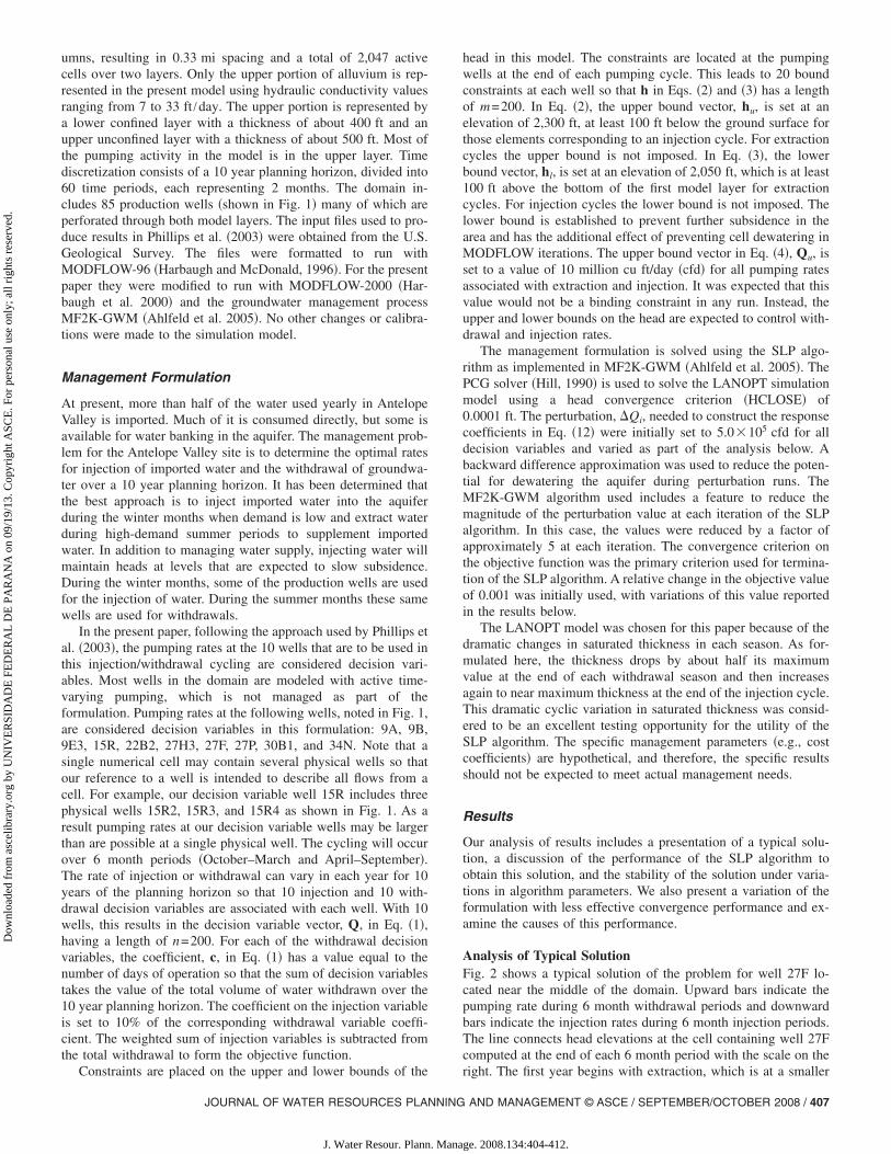
Robustness of SolutionWe next examine the robustness of the SLP algorithm undervariations in the parameters that control convergence. These pa-rameters are the set of pumping rates used to initiate the algorithmand the parameters that control the computation of the responsecoefficients supplied to the LP at each subproblem. Varying theseparameters leads to alternate trajectories of Qk iterates in the SLPalgorithm, which may affect the ability of the algorithm to con-verge. Throughout, the head is assumed to be computed to ad-equate precision to avoid significant round-off problems indetermination of the response coefficients.
Impact of Alternate Starting Points. To initiate the SLP al-gorithm an initial estimate of pumping rates, Q0, is required. Forthe results presented above the pumping rates have all been as-signed an initial value of zero. The h�Q� functions are nonlinearand may not be convex �Ahlfeld and Mulligan, 2000�. As a result,alternate local optima are possible for this problem. To examinethe potential for alternate optima and to test the robustness of theSLP algorithm we examine alternate starting points Q0.
For each alternate starting point run all pumping rates were setat the same value. These values ranged from 1.0�105 to 7.0�105. Values above this level caused the simulated aquifer todewater, and the MODFLOW flow process failed to converge.Alternate starting points produced only slight variations in results.The same pattern of active and inactive wells was obtained for allruns. The largest changes in individual pumping rates weresmaller than 1.0 cfd, and the objective function values obtainedwere different in the seventh digit. We attribute these small dif-ferences to slight differences in the computation of response co-efficients in Eq. �12� due to the different trajectory of iterates. Forthis test case, the global optimum appears to have been identified.The SLP algorithm performed well for all alternate startingpoints, converging in only four iterations for the higher-valuedstarting points that were generally closer to the optimal solution.
Impact of Perturbation Size and Direction. The responsematrix that is supplied to the LP is computed by perturbationaccording to Eq. �12�. The perturbation value, �Qi, can take anyspecified value. The perturbation parameter was varied over 4orders of magnitude from the largest practical value �2.5�106 cfd� to 5.0�103 cfd. During the SLP algorithm these val-ues were reduced by a factor of approximately 5 at each iteration.There was no discernible difference in the solutions obtained.
Fig. 6 shows the progress of the algorithm over four iterationswhen using both the forward and the backward approximationswith an initial perturbation value of 5.0�105 reduced at eachiteration by a factor of about 5. Ahlfeld and Mulligan �2000�show that the function describing the dependence of head onpumping will have a concave shape for the simple case describedby the Dupuit–Forcheimer equation for radial unconfined flow toa well. Extending this result to a more general computation ofresponses, we expect that a forward difference approximation �in-creasing withdrawal� will overestimate the drop in the head due towithdrawal while a backward difference will underestimate theresponse. This behavior can be seen in Fig. 6 where the solutionobtained with the backward difference shows more withdrawaland less injection than that obtained with the forward difference.As iterations proceed and the perturbation value decreases thesolutions converge to the same levels of withdrawal and injectionfor both the forward and the backward approximations.
Truncation error analysis indicates that smaller perturbation
values in Eq. �12� will yield more accurate approximations of the
JOURNAL OF WATER RESOURCES PLANNING
J. Water Resour. Plann. Mana
response coefficients. The importance of successively decreasingthe perturbation value, as done in the results presented here, wastested by using a constant perturbation value for all iterations ofthe SLP. These tests are summarized in Table 1 where the pertur-bation value, number of iterations to achieve convergence, andthe maximum relative deviation from base case pumping rates areshown. For all but the largest perturbation value, the differencesin solution can be attributed to round-off error in response coef-ficient computation. While only slightly different for practicalpurposes, the result for a perturbation value of 5.0�105 suggeststhat a too-large perturbation value may produce inaccurate resultsand should be avoided and that successively reducing the pertur-bation value is a useful feature of the algorithm if a large initialperturbation value is used.
Comparison with LP Solution. The importance of account-ing for the unconfined nature of the problem is demonstrated inthe results presented in Fig. 7. Here, the total pumping in eachyear and season are shown for two different solution techniques.The first set of bars �shaded and labeled as LP� represent thesolution obtained when the system is modeled as unconfined andan LP solver is used. This case would be similar to the results thatcould be obtained if a modeler chose to assume that drawdownwas small relative to saturated thickness and therefore changes in
Table 1. Impact of Different Magnitudes of Fixed Perturbation Value
Fixed perturbationvalue�cfd�
Iterations toachieve convergence
Maximum relativedeviation in
pumping rate
5.0�105 6 1.5�10−3
5.0�104 5 1.5�10−6
5.0�103 5 8.0�10−7
5.0�102 5 0.0
Fig. 6. Total withdrawal and injection volumes �cubic feet� for eachiteration of the SLP algorithm using a backward and forward approxi-mation for the response coefficient computation
thickness can be neglected. The second set of bars �black andlabeled as SLP� represent the solution obtained when the SLPsolver is used. These last bars are the results presented above. TheSLP case has consistently lower withdrawals and higher injec-tions than the LP case. This is a direct result of the increasedresponse of the head to pumping implied by accounting forchanging saturated thickness. We conclude that, for this test caseand others like it, management models that can solve the nonlin-ear optimization problem are needed.
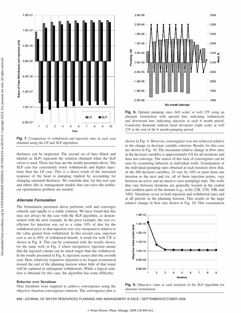
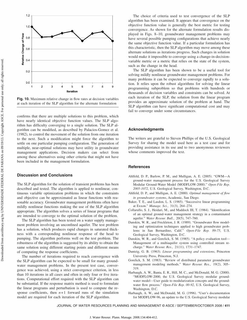
Alternate Formulation
The formulation presented above performs well and convergesrobustly and rapidly to a stable solution. We have found that thismay not always be the case with the SLP algorithm, as demon-strated with the next example. In the prior example, the cost co-efficient for injection was set to a value 10% of that for thewithdrawal price so that injection was very inexpensive relative tothe value gained from withdrawal. In this second case, injectioncost is set to 50% of withdrawal benefit. A result for well 27F isshown in Fig. 8. This can be contrasted with the results shown,for the same well, in Fig. 2 where inexpensive injection meansthat the injected volume can be much larger than the withdrawal.In the results presented in Fig. 8, injection ceases after the seventhyear. Here, relatively expensive injection is no longer economicaltoward the end of the planning horizon when little of that waterwill be captured in subsequent withdrawals. While a logical solu-tion is obtained for this case, the algorithm has some difficulty.
Behavior over IterationsNine iterations were required to achieve convergence using the
Fig. 7. Comparison of withdrawal and injection rates in each yearobtained using the LP and SLP algorithms
objective function convergence criterion. The convergence plot is
410 / JOURNAL OF WATER RESOURCES PLANNING AND MANAGEMENT
J. Water Resour. Plann. Mana
shown in Fig. 9. However, convergence was not achieved relativeto the change in decision variable criterion. Results for this caseare shown in Fig. 10. The maximum relative change in flow ratesat the decision variables is approximately 0.8 for all iterations anddoes not converge. The source of this lack of convergence can beseen by examining behavior at individual wells. Examination ofthe individual pumping rates obtained at each iteration show that,of the 200 decision variables, 24 vary by 10% or more from oneiteration to the next and six, all of them injection points, varybetween an active and an inactive �zero pumping� state. The wellsthat vary between iterations are generally located in the centraland southern parts of the domain �e.g., wells 22B, 27H, 30B, and34N�. Variations occur in both injection and withdrawal rates andat all periods in the planning horizon. This results in the largerelative change in flow rate shown in Fig. 10. This examination
Fig. 8. Optimal pumping rates �left scale� at well 27F using analternate formulation with upward bars indicating withdrawalsand downward bars indicating injection in each 6 month period.Connected diamonds indicate head elevations �right scale� at well27F at the end of the 6 month pumping period.
Fig. 9. Objective value at each iteration of the SLP algorithm foralternate formulation
confirms that there are multiple solutions to this problem, whichhave nearly identical objective function values. The SLP algo-rithm has difficulty converging to a single solution. The SLP al-gorithm can be modified, as described by Palacios-Gomez et al.�1982�, to control the movement of the solution from one iterationto the next. Such a modification might force the algorithm tosettle on one particular pumping configuration. The generation ofmultiple, near-optimal solutions may have utility in groundwatermanagement applications. Decision makers can select fromamong these alternatives using other criteria that might not havebeen included in the management formulation.
Discussion and Conclusions
The SLP algorithm for the solution of transient problems has beendescribed and tested. The algorithm is applied to nonlinear, con-tinuous variable optimization problems in which the constraintsand objective can be approximated as linear functions with rea-sonable accuracy. Groundwater management problems often havemildly nonlinear functions making the use of the SLP algorithmappropriate. The algorithm solves a series of linear programs thatare intended to converge to the optimal solution of the problem.
The SLP algorithm has been tested on a water supply manage-ment problem involving an unconfined aquifer. The test problemhas a solution, which produces rapid changes in saturated thick-ness with a corresponding nonlinear response of the head topumping. The algorithm performs well on the test problem. Therobustness of the algorithm is suggested by its ability to obtain thesame solution using different starting points and different meansof computing the response coefficients.
The number of iterations required to reach convergence withthe SLP algorithm can be expected to be small for many ground-water management problems. In the present test case, conver-gence was achieved, using a strict convergence criterion, in lessthan 10 iterations in all cases and often in only four or five itera-tions. Computational effort required with the SLP algorithm canbe substantial. If the response matrix method is used to formulatethe linear programs and perturbation is used to compute the re-sponse coefficients, then n+1 forward runs of the simulation
Fig. 10. Maximum relative change in flow rates at decision variablesat each iteration of the SLP algorithm for the alternate formulation
model are required for each iteration of the SLP algorithm.
JOURNAL OF WATER RESOURCES PLANNING
J. Water Resour. Plann. Mana
The choice of criteria used to test convergence of the SLPalgorithm has been examined. It appears that convergence on theobjective function value is generally the best metric for testingconvergence. As shown for the alternate formulation results dis-played in Figs. 8–10, groundwater management problems mayhave several possible pumping configurations that achieve nearlythe same objective function value. If a particular formulation hasthis characteristic, then the SLP algorithm may move among thesealternate solutions as iterations progress. Such changes in solutionwould make it impossible to converge using a change-in-decision-variable metric or a metric that relies on the state of the system,such as the change in the head.
The SLP algorithm has been shown to be a useful tool forsolving mildly nonlinear groundwater management problems. Formany problems it can be expected to converge rapidly to a solu-tion. It relies upon the robust algorithms for solving the linearprogramming subproblem so that problems with hundreds orthousands of decision variables and constraints can be solved. Ateach iteration of the SLP, the solution from the linear programprovides an approximate solution of the problem at hand. TheSLP algorithm can have significant computational cost and mayfail to converge under some circumstances.
Acknowledgments
The writers are grateful to Steven Phillips of the U.S. GeologicalSurvey for sharing the model used here as a test case and forproviding assistance in its use and to two anonymous reviewerswhose comments improved the text.
References
Ahlfeld, D. P., Barlow, P. M., and Mulligan, A. E. �2005�. “GWM—Aground-water management process for the U.S. Geological SurveyModular Ground-Water Model �MODFLOW-2000�.” Open-File Rep.2005-1072, U.S. Geological Survey, Washington, D.C.
Ahlfeld, D. P., and Mulligan, A. E. �2000�. Optimal management of flowin groundwater systems, Academic, San Diego.
Baker, T. E., and Lasdon, L. S. �1985�. “Successive linear programmingat Exxon.” Manage. Sci., 31�3�, 264–274.
Collarullo, S. J., Heidari, M., and Maddock III, T. �1984�. “Identificationof an optimal ground-water management strategy in a contaminatedaquifer.” Water Resour. Bull., 20�5�, 747–760.
Danskin, W. R., and Freckleton, J. R. �1989�. “Groundwater flow model-ing and optimization techniques applied to high groundwater prob-lems in San Bernardino, Calif.” Open-File Rep. 89-75, U.S.Geological Survey, Washington, D.C.
Danskin, W. R., and Gorelick, S. M. �1985�. “A policy evaluation tool—Management of a multiaquifer system using controlled stream re-charge.” Water Resour. Res., 21�11�, 1731–1747.
Dantzig, G. B. �1963�. Linear programming and extensions, PrincetonUniversity Press, Princeton, N.J.
Gorelick, S. M. �1983�. “Review of distributed parameter groundwatermanagement modeling methods.” Water Resour. Res., 19�2�, 305–319.
Harbaugh, A. W., Banta, E. R., Hill, M. C., and McDonald, M. G. �2000�.“MODFLOW-2000, the U.S. Geological Survey modular ground-water model—User guide to modularization concepts and the ground-water flow process.” Open-File Rep. 00-92, U.S. Geological Survey,Washington, D.C.
Harbaugh, A. W., and McDonald, M. G. �1996�. “User’s documentation
for MODFLOW-96, an update to the U.S. Geological Survey modular
Hill, M. C. �1990�. “Preconditioned conjugate-gradient 2 �PCG2�, a com-puter program for solving ground-water flow equations.” Water-Resources Investigations Rep. 90-4048, U.S. Geological Survey,Washington, D.C.
Hsiao, C. T., and Chang, L. C. �2005�. “Optimizing remediation of anunconfined aquifer using a hybrid algorithm.” Ground Water, 43�6�,904–915.
Ikehara, M. E., and Phillips, S. P. �1994�. “Determination of land subsid-ence related to ground-water-level declines using GPS and levelingsurveys in Antelope Valley, Los Angeles and Kern Counties, Calif.1992.” Water Resources Investigations Rep. 1994-4184, U.S. Geologi-cal Survey, Washington, D.C.
Jones, L., Willis, R., and Yeh, W. W.-G. �1987�. “Optimal control ofnonlinear groundwater hydraulics using differential dynamic pro-gramming.” Water Resour. Res., 23�11�, 2097–2106.
Kosmidis, V. D., Perkins, J. D., and Pistikopoulos, E. N. �2004�. “Opti-mization of well oil rate allocations in petroleum fields.” Ind. Eng.Chem. Res., 43�14�, 3513–3527.
Leighton, D., and Phillips, S. P. �2003�. “Simulation of ground-water flowand land subsidence in the Antelope Valley ground-water basin,Calif.” Water Resources Investigation Rep. 2003-4016, U.S. Geologi-cal Survey, Washington, D.C.
Mansfield, C. M., and Shoemaker, C. A. �1999�. “Optimal remediation ofunconfined aquifers: Numerical applications and derivative calcula-tions.” Water Resour. Res., 35�5�, 1455–1469.
Mayer, A. S., Kelley, C. T., and Miller, C. T. �2002�. “Optimal design forproblems involving flow and transport phenomena in saturated sub-surface systems.” Adv. Water Resour., 25�8–12�, 1233–1256.
412 / JOURNAL OF WATER RESOURCES PLANNING AND MANAGEMENT
J. Water Resour. Plann. Mana
Palacios-Gomez, F., Lasdon, L., and Engquist, M. �1982�. “Non-linearoptimization by successive linear programming.” Manage. Sci.,28�10�, 1106–1120.
Phillips, S. P., Carlson, C. S., Metzger, L. F., Howle, J. F., Galloway, D.L., Sneed, M., Ikehara, M. E., Hudnut, K. W., and King, N. �2003�.“Analysis of tests of subsurface injection, storage, and recovery offreshwater in Lancaster, Antelope Valley, Calif.” Water Resources In-vestigation Rep., 2003-4061, U.S. Geological Survey, Washington,D.C.
Stewart, R. A., and Griffith, R. E. �1961�. “A nonlinear programmingtechnique for the optimization of continuous processing systems.”Manage. Sci., 7�4�, 359–392.
Tao, T., and Lennox, W. C. �1991�. “Reservoir operations by successivelinear-programming.” J. Water Resour. Plann. Manage., 117�2�, 274–280.
Tokgoz, M., Yilmaz, K. K., and Yazicigil, H. �2002�. “Optimal aquiferdewatering schemes for excavation of collector line.” J. Water Resour.Plann. Manage., 128�4�, 248–261.
Vedula, S., Mujumdar, P. P., and Sekhar, G. C. �2005�. “Conjunctive usemodeling for multicrop irrigation.” Agric. Water Manage., 73�3�,193–221.
Wagner, B. J. �1995�. “Recent advances in simulation-optimizationgroundwater management modeling.” Rev. Geophys., 33�S1�, 1021–1028.
Willis, R., and Finney, B. A. �1985�. “Optimal control of nonlineargroundwater hydraulics: Theoretical development and numerical ex-periments.” Water Resour. Res., 21�10�, 1476–1482.
Yeh, W. W.-G. �1992�. “Systems analysis in groundwater planning andmanagement.” J. Water Resour. Plann. Manage., 118�1�, 224–237.