Some Associations between Arctic Sea Level Pressure and

RemotePhenomena Seen in Daily Data

Richard GrotjahnDept. of Land, Air, & Water Resources,

University of California, Davis

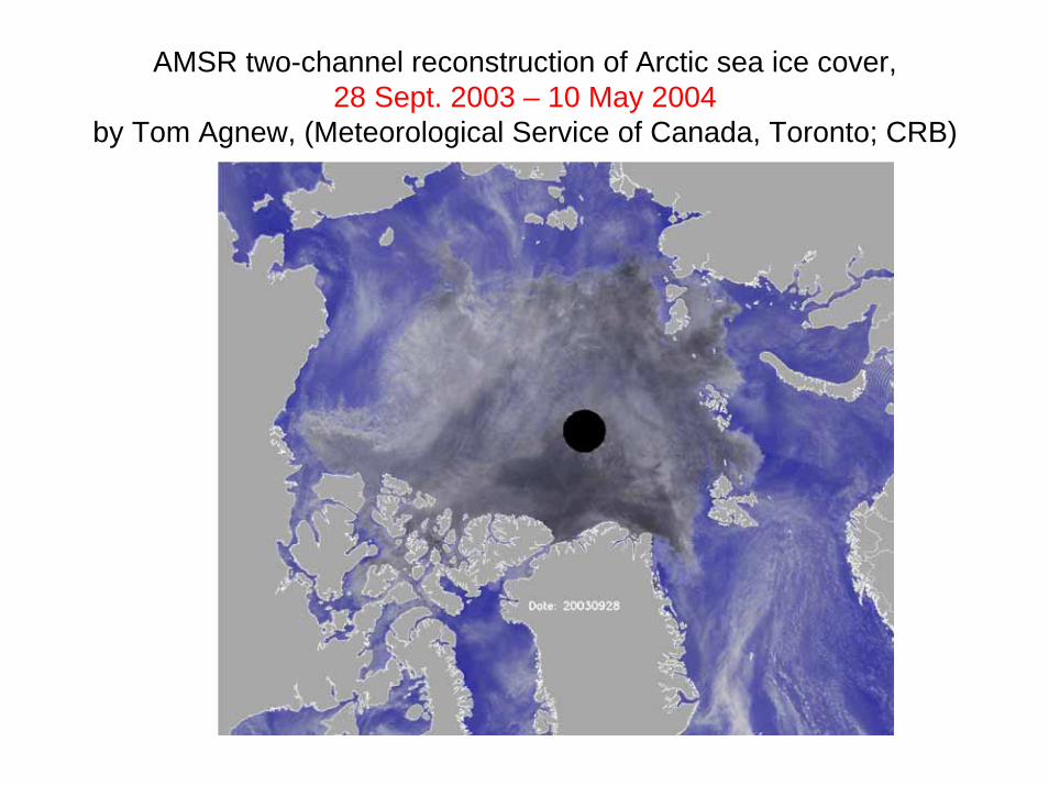
AMSR two-channel reconstruction of Arctic sea ice cover, 28 Sept. 2003 – 10 May 2004

by Tom Agnew, (Meteorological Service of Canada, Toronto; CRB)

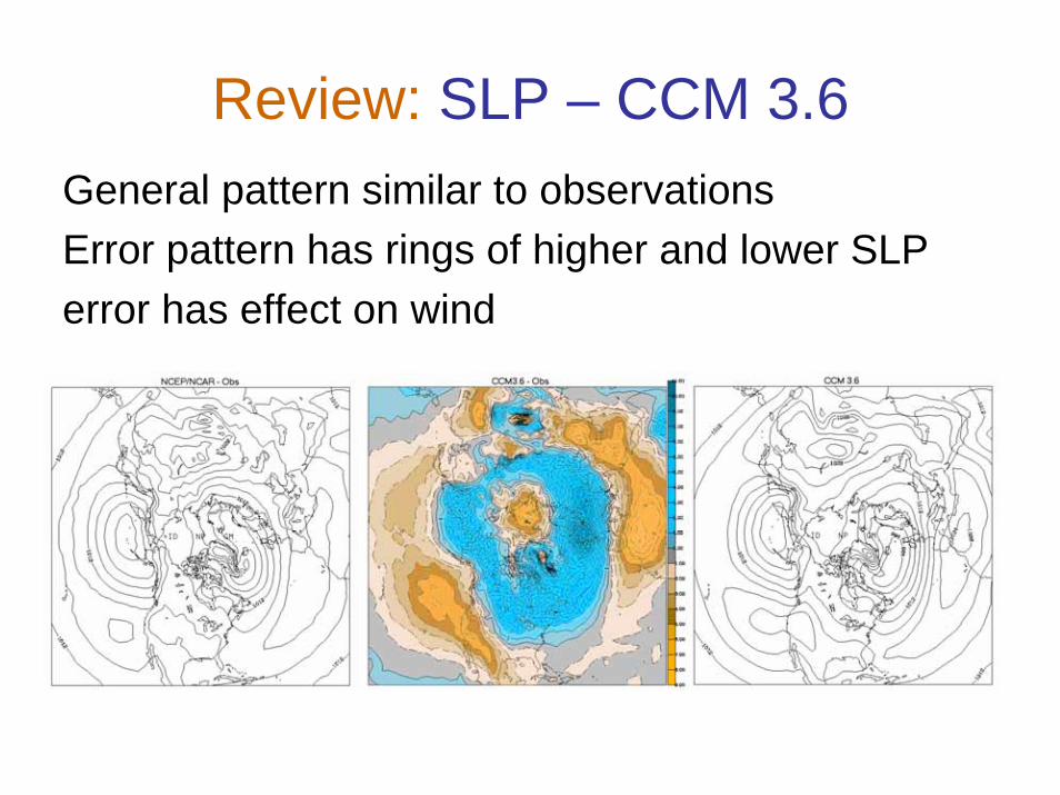
Review: SLP – CCM 3.6General pattern similar to observationsError pattern has rings of higher and lower SLPerror has effect on wind

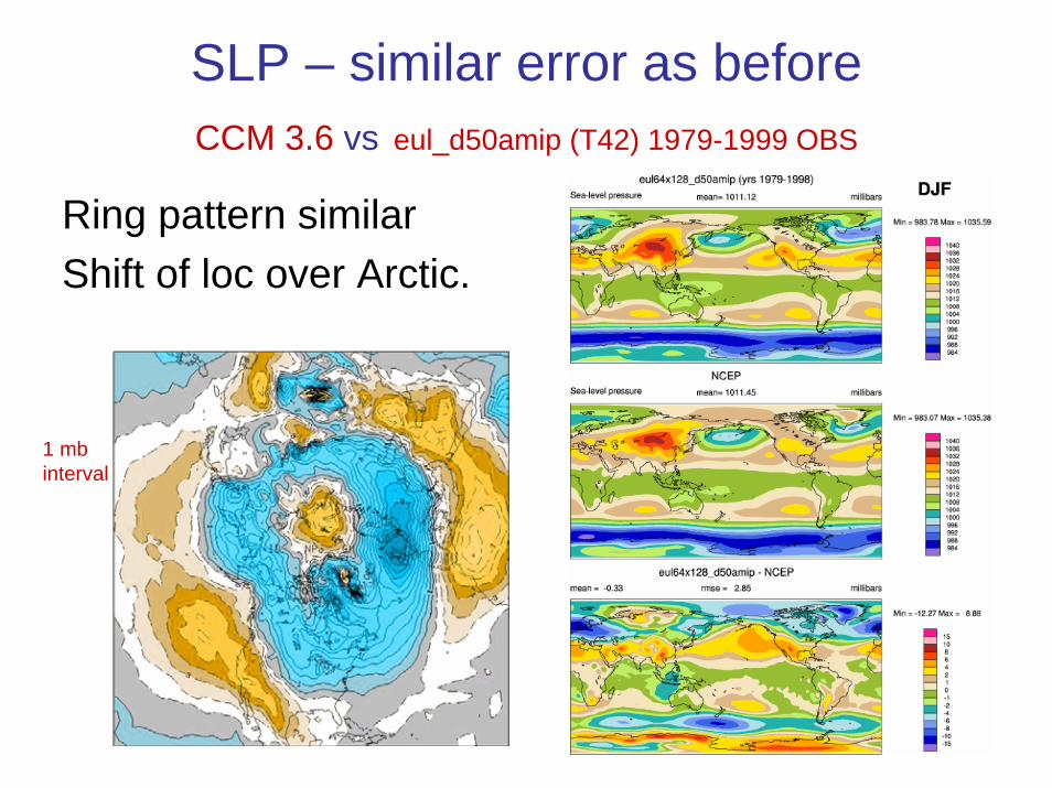
SLP – similar error as beforeCCM 3.6 vs eul_d50amip (T42) 1979-1999 OBS

Ring pattern similarShift of loc over Arctic.

1 mbinterval

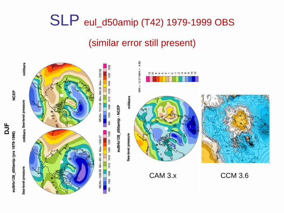
SLP eul_d50amip (T42) 1979-1999 OBS

(similar error still present)

CCM 3.6CAM 3.x

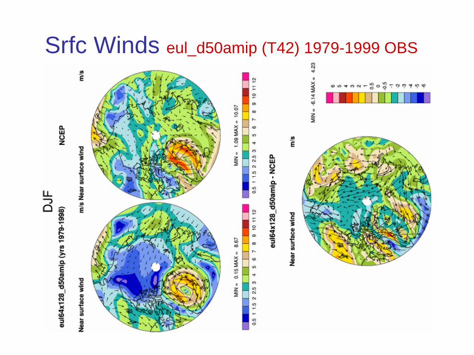
Srfc Winds eul_d50amip (T42) 1979-1999 OBS

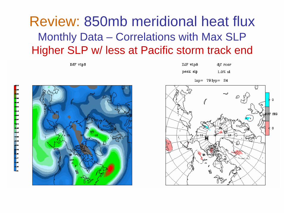
Review: 850mb meridional heat fluxMonthly Data – Correlations with Max SLP

Higher SLP w/ less at Pacific storm track end

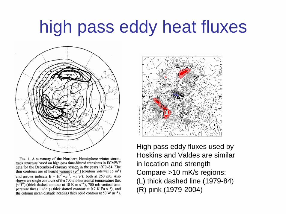
high pass eddy heat fluxes

High pass eddy fluxes used by Hoskins and Valdes are similar in location and strengthCompare >10 mK/s regions:(L) thick dashed line (1979-84)(R) pink (1979-2004)

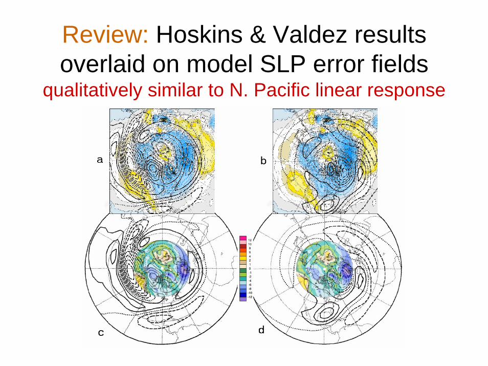
Review: Hoskins & Valdez results overlaid on model SLP error fields

qualitatively similar to N. Pacific linear response

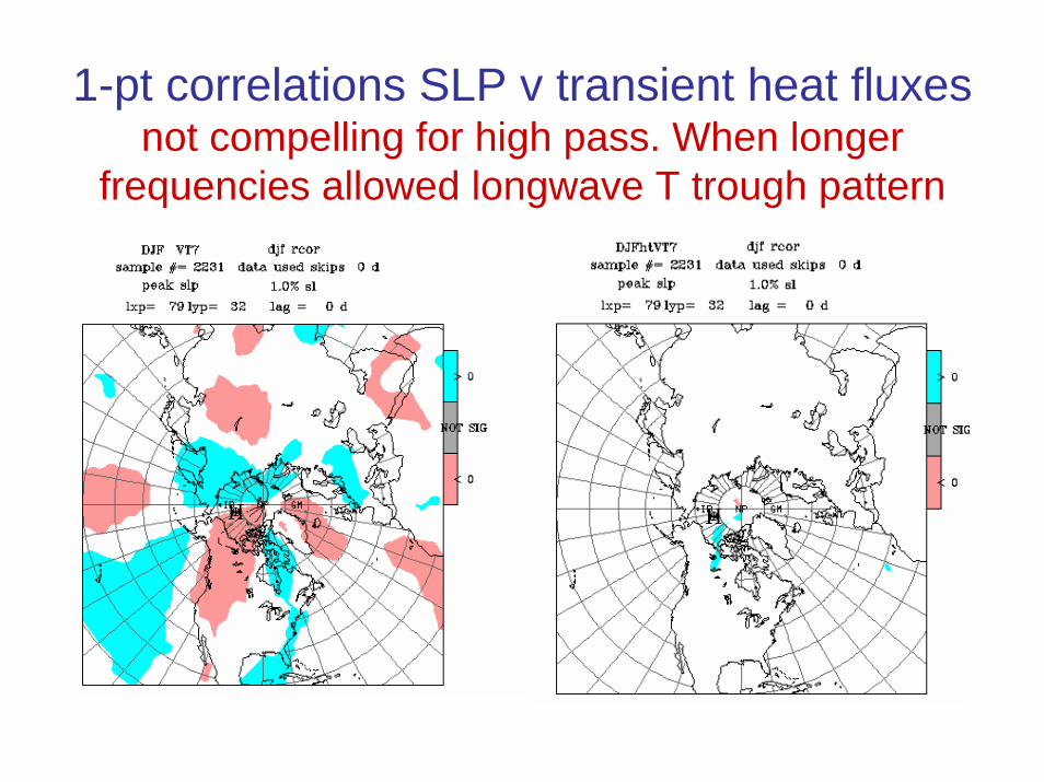
1-pt correlations SLP v transient heat fluxes not compelling for high pass. When longer

frequencies allowed longwave T trough pattern

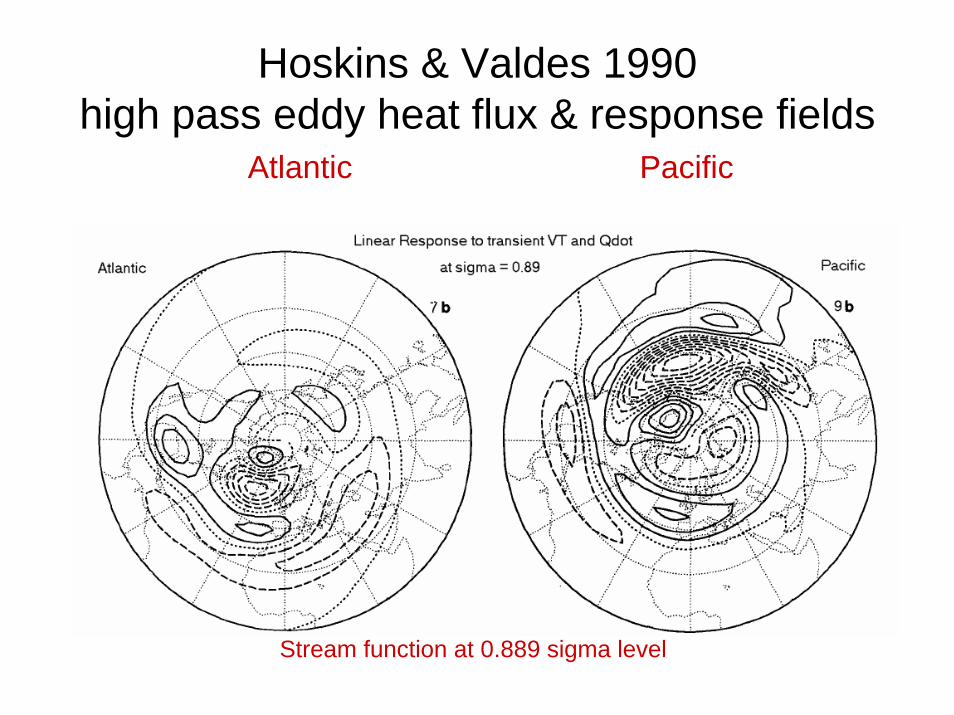
Hoskins & Valdes 1990high pass eddy heat flux & response fields

Atlantic Pacific

Stream function at 0.889 sigma level

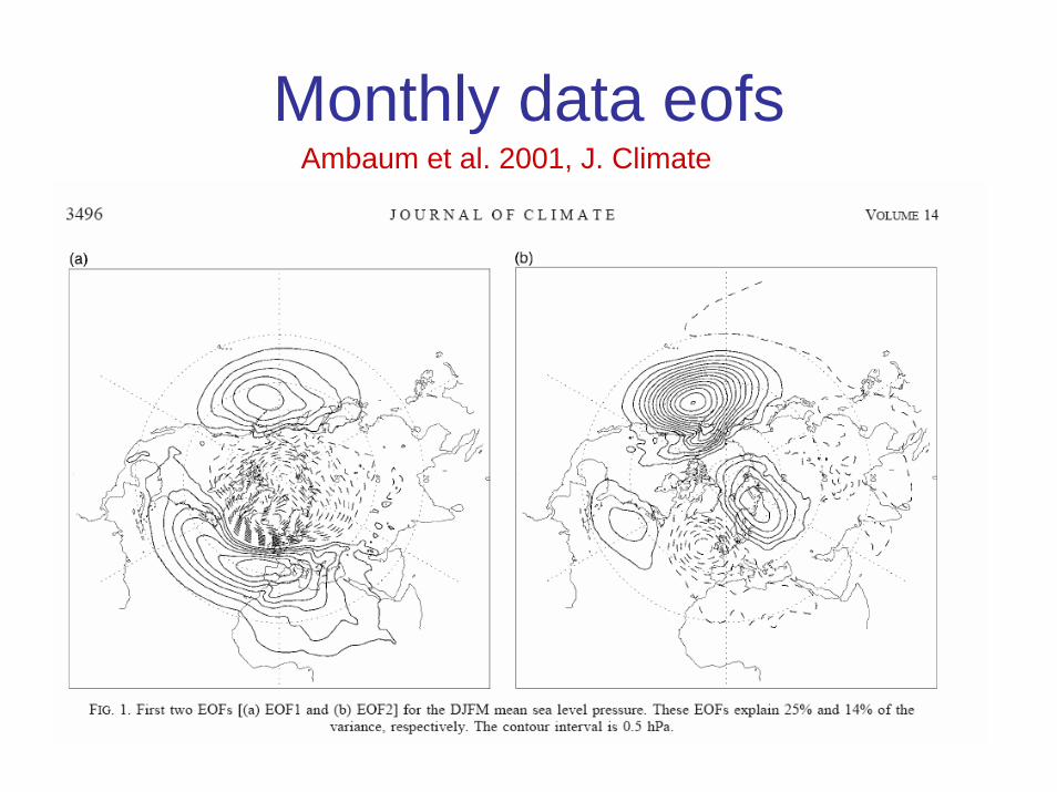
Monthly data eofsAmbaum et al. 2001, J. Climate

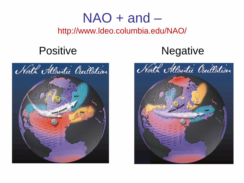
NAO + and –http://www.ldeo.columbia.edu/NAO/

Positive Negative

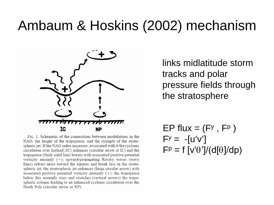
Ambaum & Hoskins (2002) mechanism

links midlatitude storm tracks and polar pressure fields through the stratosphere

EP flux = (Fy , Fp )Fy = -[u’v’] Fp = f [v’θ’]/(d[θ]/dp)

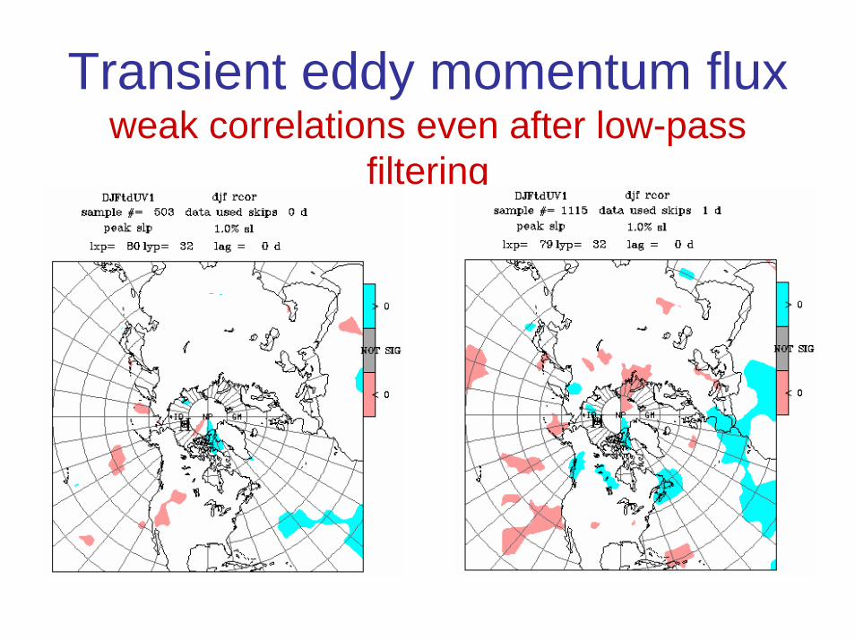
Transient eddy momentum fluxweak correlations even after low-pass

filtering

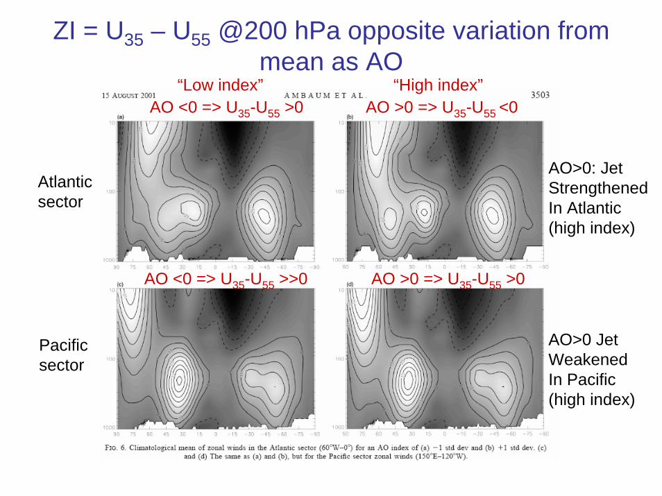
ZI = U35 – U55 @200 hPa opposite variation from mean as AO

AO <0 => U35-U55 >0

Atlanticsector

Pacificsector

AO <0 => U35-U55 >>0 AO >0 => U35-U55 >0

AO >0 => U35-U55 <0

AO>0: Jet StrengthenedIn Atlantic(high index)

AO>0 Jet WeakenedIn Pacific(high index)

“High index”“Low index”

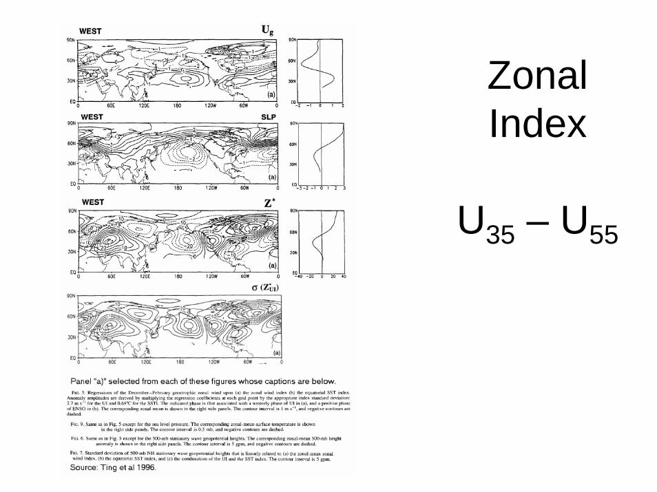
ZonalIndex

U35 – U55

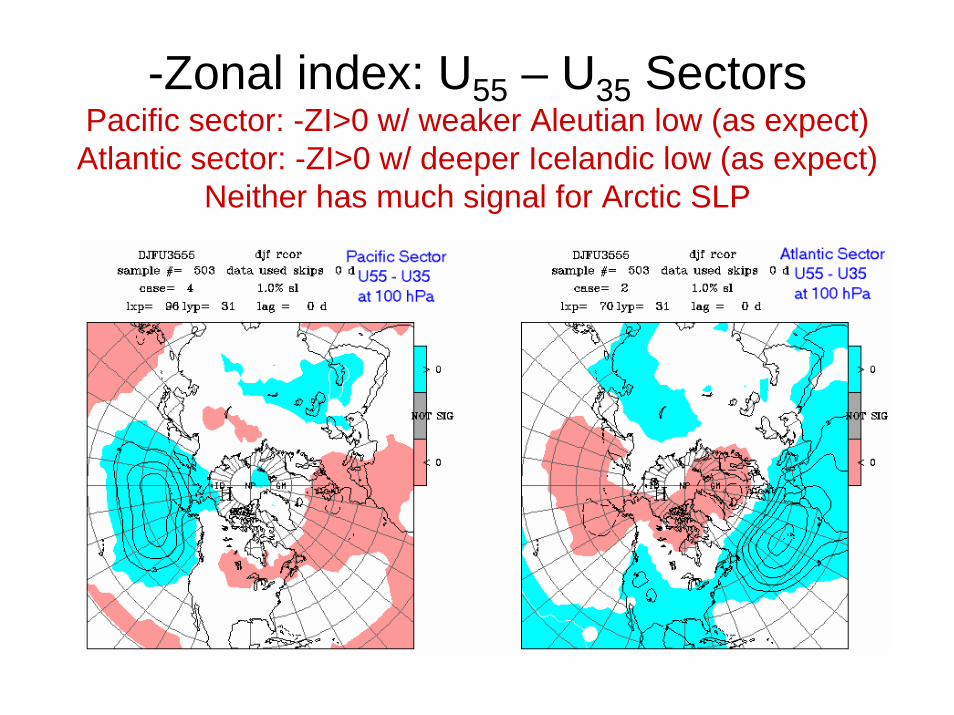
-Zonal index: U55 – U35 SectorsPacific sector: -ZI>0 w/ weaker Aleutian low (as expect)Atlantic sector: -ZI>0 w/ deeper Icelandic low (as expect)

Neither has much signal for Arctic SLP

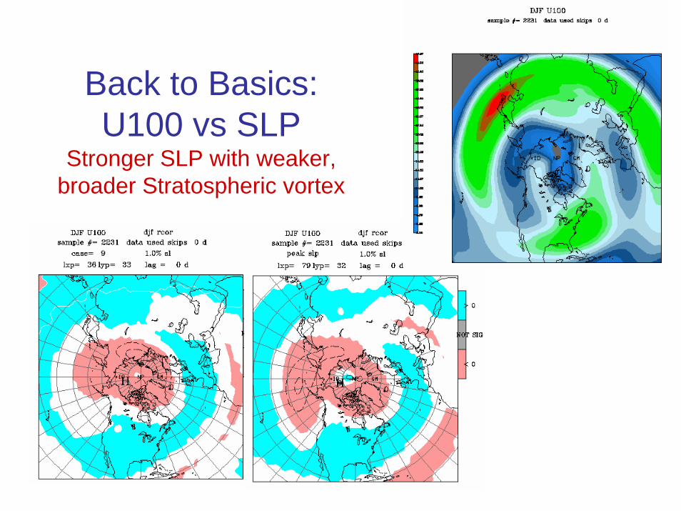
Back to Basics: U100 vs SLP

Stronger SLP with weaker, broader Stratospheric vortex

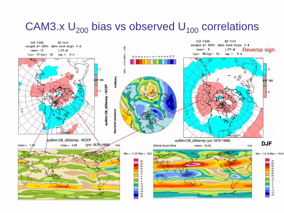
CAM3.x U200 bias vs observed U100 correlations

Reverse sign

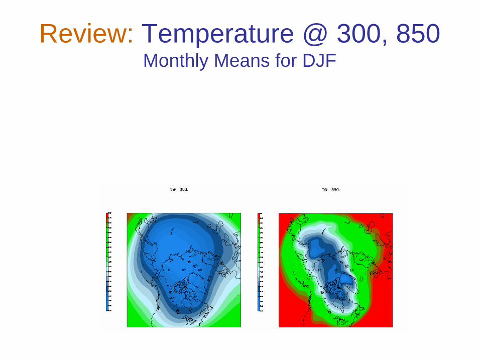
Review: Temperature @ 300, 850Monthly Means for DJF

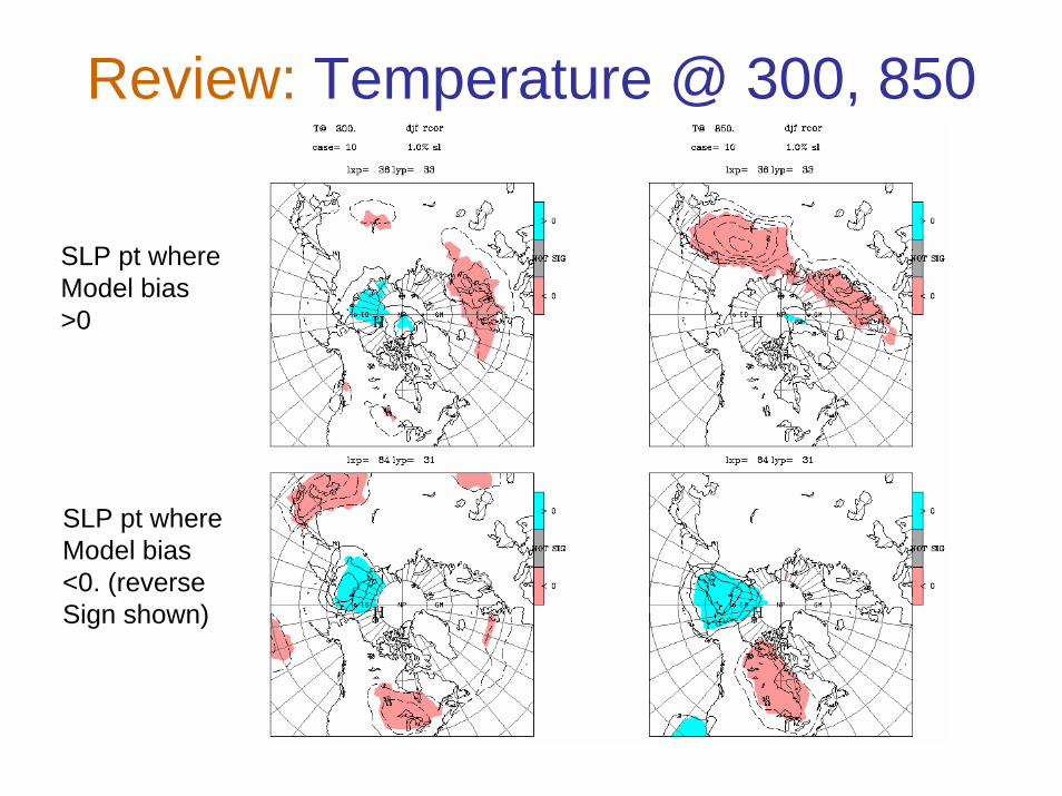
Review: Temperature @ 300, 850

SLP pt whereModel bias >0

SLP pt whereModel bias <0. (reverseSign shown)

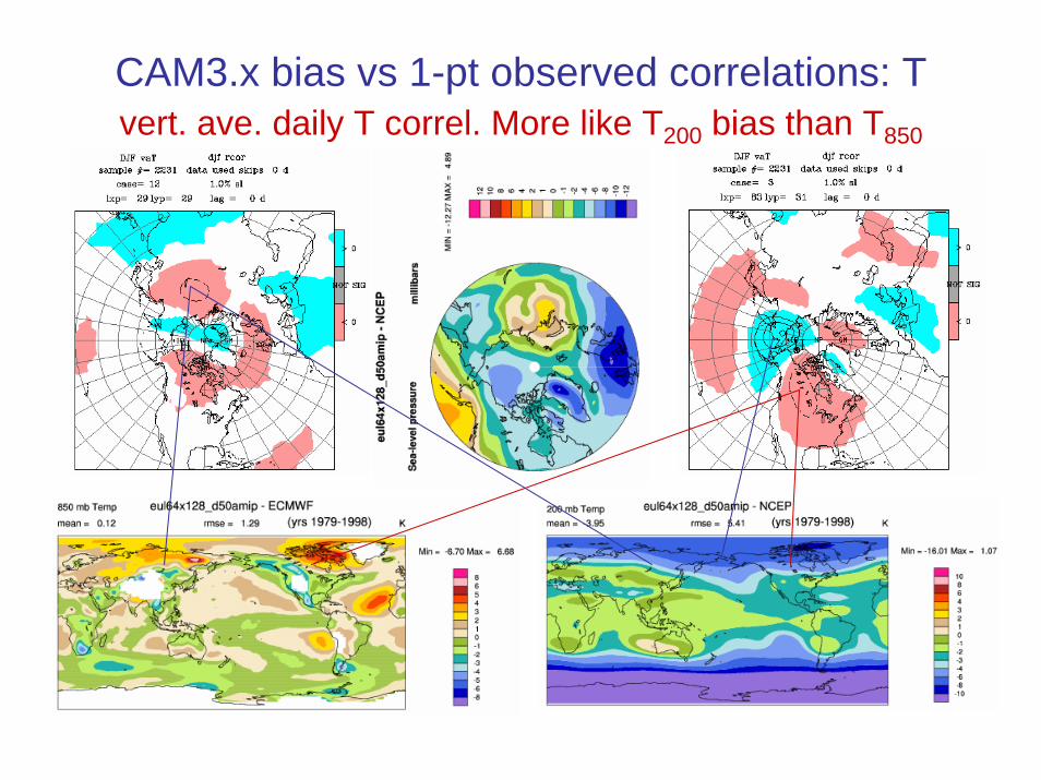
CAM3.x bias vs 1-pt observed correlations: Tvert. ave. daily T correl. More like T200 bias than T850

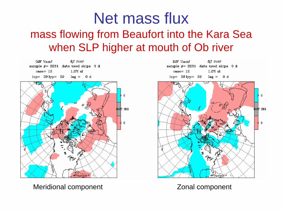
Net mass fluxmass flowing from Beaufort into the Kara Sea

when SLP higher at mouth of Ob river

Meridional component Zonal component

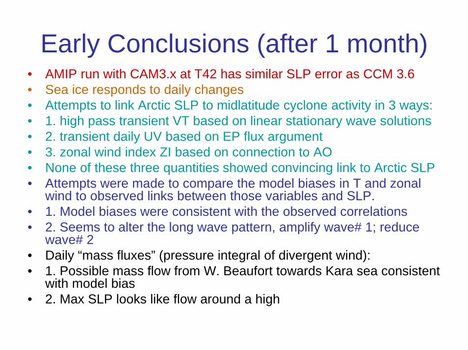
Early Conclusions (after 1 month)• AMIP run with CAM3.x at T42 has similar SLP error as CCM 3.6• Sea ice responds to daily changes• Attempts to link Arctic SLP to midlatitude cyclone activity in 3 ways: • 1. high pass transient VT based on linear stationary wave solutions• 2. transient daily UV based on EP flux argument• 3. zonal wind index ZI based on connection to AO• None of these three quantities showed convincing link to Arctic SLP• Attempts were made to compare the model biases in T and zonal

wind to observed links between those variables and SLP. • 1. Model biases were consistent with the observed correlations• 2. Seems to alter the long wave pattern, amplify wave# 1; reduce

wave# 2• Daily “mass fluxes” (pressure integral of divergent wind):• 1. Possible mass flow from W. Beaufort towards Kara sea consistent

with model bias• 2. Max SLP looks like flow around a high

Future Work• Consult with collaborators• Additional observational work: diabatic heating,

composites• Better eddy flux information, possibly with filtering • Further comparison of model fields to parallel the

observational work• Test stationary wave model response to prescribed

anomalous: eddy fluxes, diabatic heating (“stationary wave model”)

• Test what anomalous eddy fluxes arise from an anomalous stationary wave pattern (“storm track model”)

• Model variations (topography, surface stress, etc.)

Storage

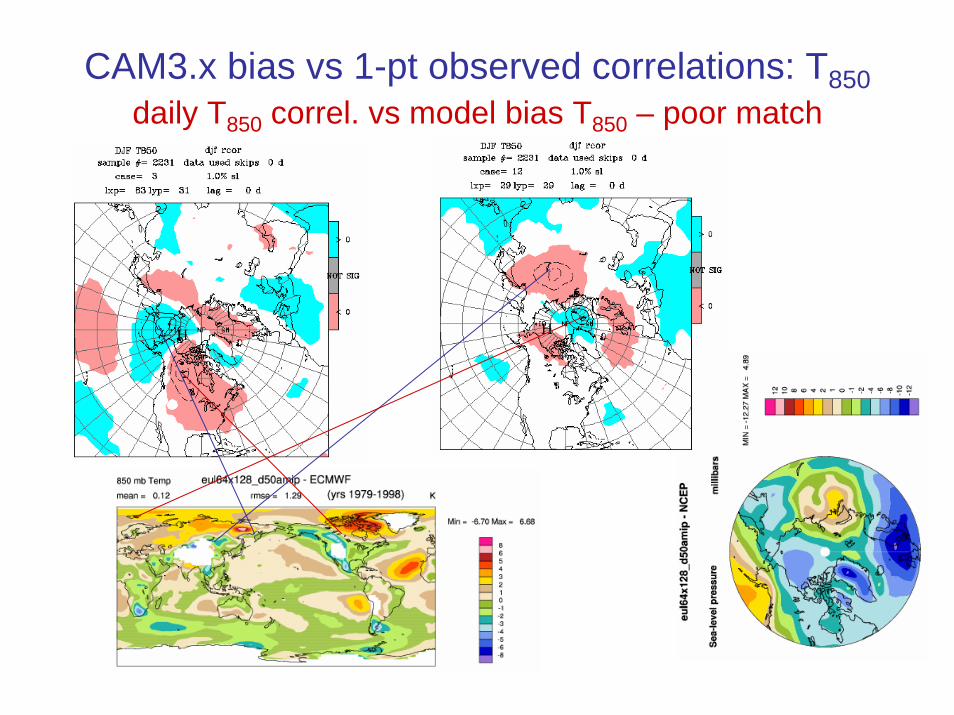
CAM3.x bias vs 1-pt observed correlations: T850daily T850 correl. vs model bias T850 – poor match

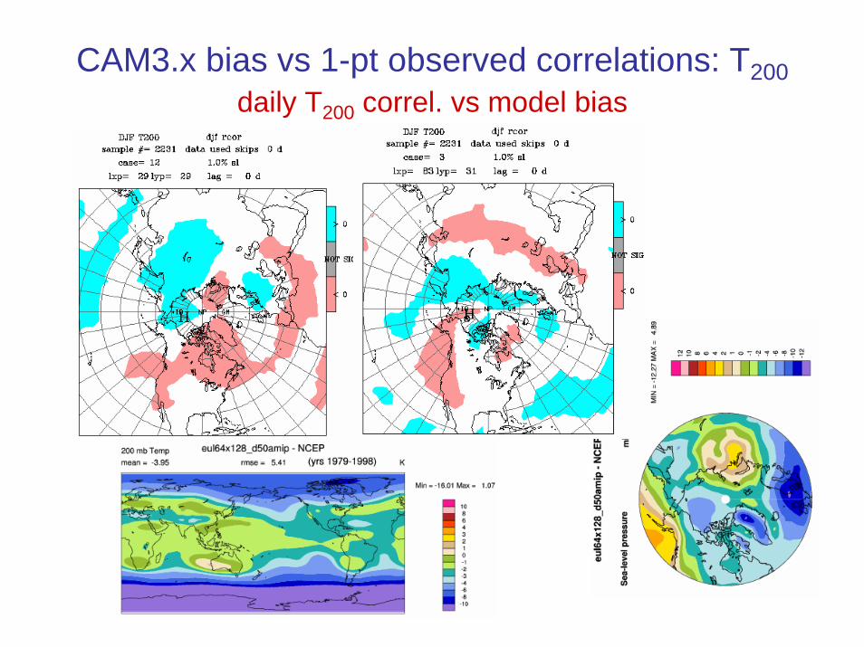
CAM3.x bias vs 1-pt observed correlations: T200daily T200 correl. vs model bias

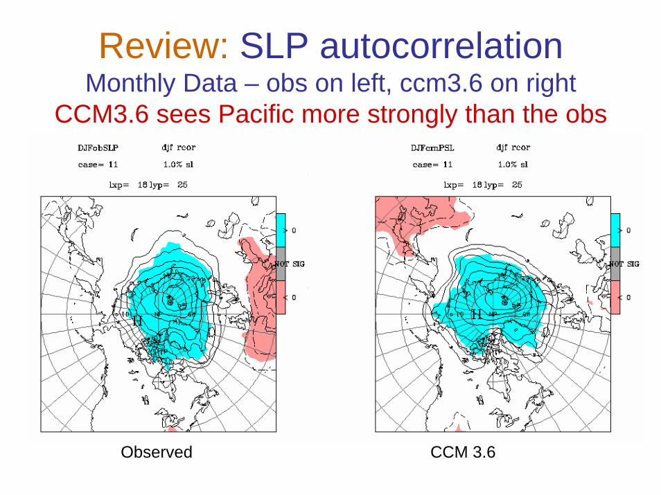
Review: SLP autocorrelationMonthly Data – obs on left, ccm3.6 on right

CCM3.6 sees Pacific more strongly than the obs

Observed CCM 3.6

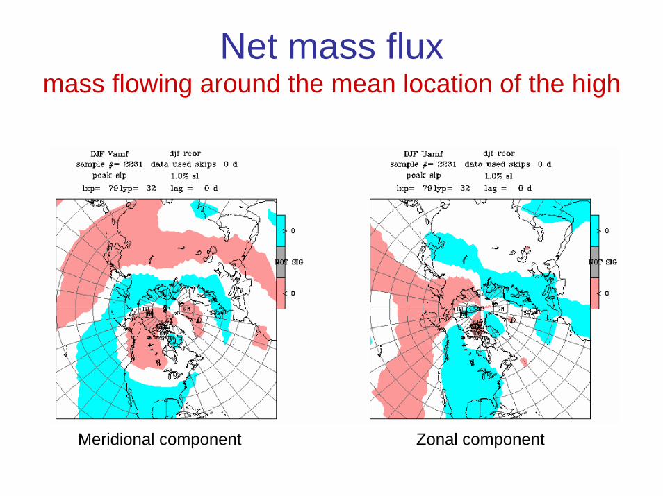
Net mass fluxmass flowing around the mean location of the high

Meridional component Zonal component

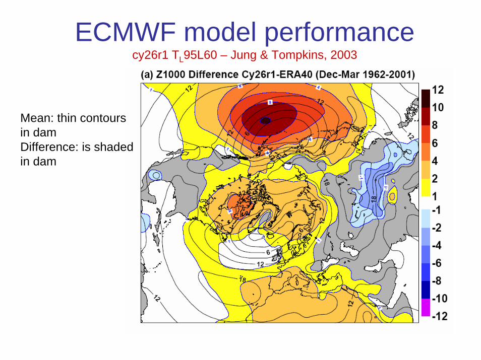
ECMWF model performancecy26r1 TL95L60 – Jung & Tompkins, 2003

Mean: thin contours in damDifference: is shaded in dam

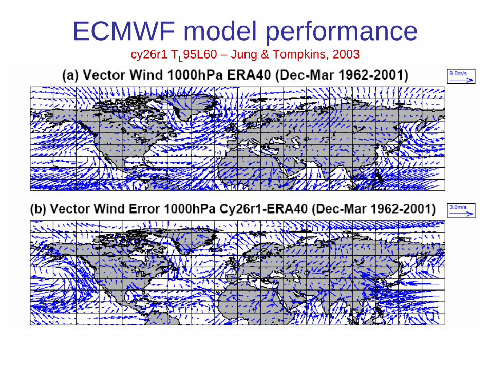
ECMWF model performancecy26r1 TL95L60 – Jung & Tompkins, 2003