Some Characteristics of Open Channel Transition Flow

AKM Enamul Haque

A Thesis

In

The Department

of

Building, Civil, and Environmental Engineering

Presented in Partial Fulfillment of the Requirements

for the Degree of Master of Applied Science in Civil Engineering at

Concordia University

Montreal, Quebec, Canada

September, 2008

©AKM Enamul Haque, 2008

1*1 Library and Archives Canada

Published Heritage Branch

395 Wellington Street OttawaONK1A0N4 Canada

Bibliotheque et Archives Canada

Direction du Patrimoine de ('edition

395, rue Wellington Ottawa ON K1A 0N4 Canada

Your file Votre reference ISBN: 978-0-494-63268-0 Our file Notre reference ISBN: 978-0-494-63268-0

NOTICE: AVIS:

The author has granted a non­exclusive license allowing Library and Archives Canada to reproduce, publish, archive, preserve, conserve, communicate to the public by telecommunication or on the Internet, loan, distribute and sell theses worldwide, for commercial or non­commercial purposes, in microform, paper, electronic and/or any other formats.

L'auteur a accorde une licence non exclusive permettant a la Bibliotheque et Archives Canada de reproduire, publier, archiver, sauvegarder, conserver, transmettre au public par telecommunication ou par I'lnternet, preter, distribuer et vendre des theses partout dans le monde, a des fins commerciales ou autres, sur support microforme, papier, electronique et/ou autres formats.

The author retains copyright ownership and moral rights in this thesis. Neither the thesis nor substantial extracts from it may be printed or otherwise reproduced without the author's permission.

L'auteur conserve la propriete du droit d'auteur et des droits moraux qui protege cette these. Ni la these ni des extraits substantiels de celle-ci ne doivent etre imprimes ou autrement reproduits sans son autorisation.

In compliance with the Canadian Privacy Act some supporting forms may have been removed from this thesis.

Conformement a la loi canadienne sur la protection de la vie privee, quelques formulaires secondaires ont ete enleves de cette these.

While these forms may be included in the document page count, their removal does not represent any loss of content from the thesis.

Bien que ces formulaires aient inclus dans la pagination, il n'y aura aucun contenu manquant.

1+1

Canada

I l l

ABSTRACT

Some Characteristics of Open Channel Transition Flow

AKM Enamul Haque

Flow separation is a common phenomenon in decelerated subcritical flows as in open

channel expansions. A highly distorted velocity and shear stress distribution due to flow

separation can lead to a continuous reduction of energy and trigger an adverse pressure

gradient resulting in flow separation. This causes loss of energy and hydraulic efficiency

of the systems. An experimental investigation was conducted with the use of a gradual

rising hump on the bed of an expansion in a rectangular open channel. Besides the hump,

split vanes in the flow field were also used to reduce the expansion angle and in turn

reduce the adverse effect of flow separation. These modifications resulted in a relatively

more uniform velocity and shear stress distribution in the transition and in the channel

downstream of the expansion.

A laboratory model of rectangular open channel transition expanding was constructed

with Plexiglas plates. It facilitated the measurement of the flow velocity and turbulence

characteristics with the aid of Laser Doppler Anemometer (LDA). The total divergent

angle of the transition was 19.78 degrees. Velocities were measured along the x, y and z

directions, positioning the LDA from both the bottom and the side of the channel.

iv

Two humps with gradual linear rises of 12.5 mm and 25 mm were used. A second device

included the use of a single vane and a three vane splitter plates system formed with thin

Plexiglas plates.

Mainly velocity distributions, with and without humps and the splitter vanes were the

results sought. The variations of energy and momentum coefficients were analyzed to

find the effectiveness of the devices used in the transition to control flow separation.

As a small addition to the study, the use of computational fluid dynamics (CFD) to

predict the flow characteristics of open channel was also undertaken. Due to their lower

time demand and lower cost, these numerical methods are preferred to experimental

methods after they are properly validated. In the present study, the CFD solution is

validated by experimental results. A limited number of CFD simulations were completed

using the commercial Software ANSYS-CFX. In particular, mean velocity distributions

for the rectangular open channel transitions were used for model validation. To this end,

the three-dimensional Reynolds-Averaged Navier-Stokes (RANS) equations and the two

equations k-s models were used. The validation of the model using test data was

reasonable.

V

ACKNOWLEDGEMENT

I wish to thank Dr. A. S. Ramamurthy for suggesting this research work. I would also like

to express my gratitude to Mr. Mustafa Azmal, PhD student and Dr. Diep VO for their

assistance and cooperation while conducting the tests in the laboratory.

I would like to thank the doctoral students Mr. Sangsoo Han and Mr. Rahim Tadayan for

their helpful suggestions during the course of this research. I am also grateful to Mr. Lang

Vo who helped me to install the laboratory set up for this study. Thanks are also due to

friends and all those who helped me to carry out this study.

Last but not the least, I express my deepest gratitude and appreciation to my wife

Shahana, son Naveed and daughter Nawreen for their patience, understanding and

unfailing support.

vi

TABLE OF CONTENTS

List of Figures x

List of Tables xii

List of Symbols xiii

CHAPTER 1 INTRODUCTION 1

1.1 General remarks 1

1.2 Objective of the study 2

1.3 Scope of the study 3

CHAPTER 2 LITERATURE REVIEW 5

2.1 Flow separation mechanism 5

2.2 Boundary layer flow 7

2.3 Losses in open channel 9

2.4 Turbulence characteristics in channel transition 12

2.5 Geometry of divergence to control flow separation 13

2.6 Design considerations for transitions 15

2.7 Method of control of flow separation 16

2.8 Some previous method of design 19

2.9 Present study related to flow separation in rectangular

open channel transitions 20

vii

CHAPTER 3 EXPERIMENTAL SETUP 26

3.1 Physical Model 26

3.1.1 Experimental Channel 26

3.2Instrumentation 29

3.2.1 Velocity Measurements 29

3.2.2 Depth Measurements 32

3.2.3 Pressure Head Measurements 32

3.2.4 Other Measurements 33

CHAPTER 4 THEORETICAL CONSIDERATIONS 33

4.1 Hump and its effects 34

4.2 Velocity coefficient 36

4.3 Energy efficiency in diverging flows 37

4.3.1 General approach 37

4.3.2 Diffuser effectiveness 37

4.3.3 Turbulence intensity and turbulent kinetic energy 38

4.3.4 Boundary shear stress distribution 39

4.3.5 The Reynolds number 40

4.3.6 Froude number 40

CHAPTER 5 3D NUMERICAL SIMULATION 42

5.1 CFD modeling 42

5.2 Computational fluid dynamics (CFD) 42

viii

5.3 Organization of CFD codes 44

5.4.0 Basic governing equations 45

5.4.1 Navier-Stokes equation 45

5.4.2 Two-equation model k-s and k-co 46

5.4.3 Boundary conditions 47

5.4.4 Inlet boundaries 48

5.4.5 Outlet boundaries 48

5.4.6 Free surface boundaries 48

5.4.7 Interface-tracking scheme 48

5.4.8 Interface-capturing scheme 49

5.4.9 Wall function 50

5.4.10 Grid generation 50

CHAPTER 6 DISCUSSION OF RESULTS 51

6.1.0 Experimental results 51

6.1.1 The Reynolds number effect 52

6.1.2 The Energy o-efficient a and momentum co-efficient P 53

6.1.3 Velocity distribution and percentage

area of reversal flow 55

6.1.4 Transition flow characteristics with a hump 56

6.1.5 Effect of vane on transition flow characteristics 56

6.1.6 Turbulent kinetic energy and turbulence intensities 57

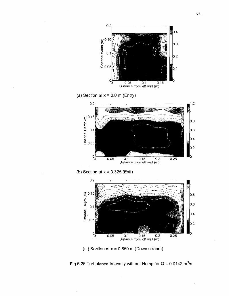
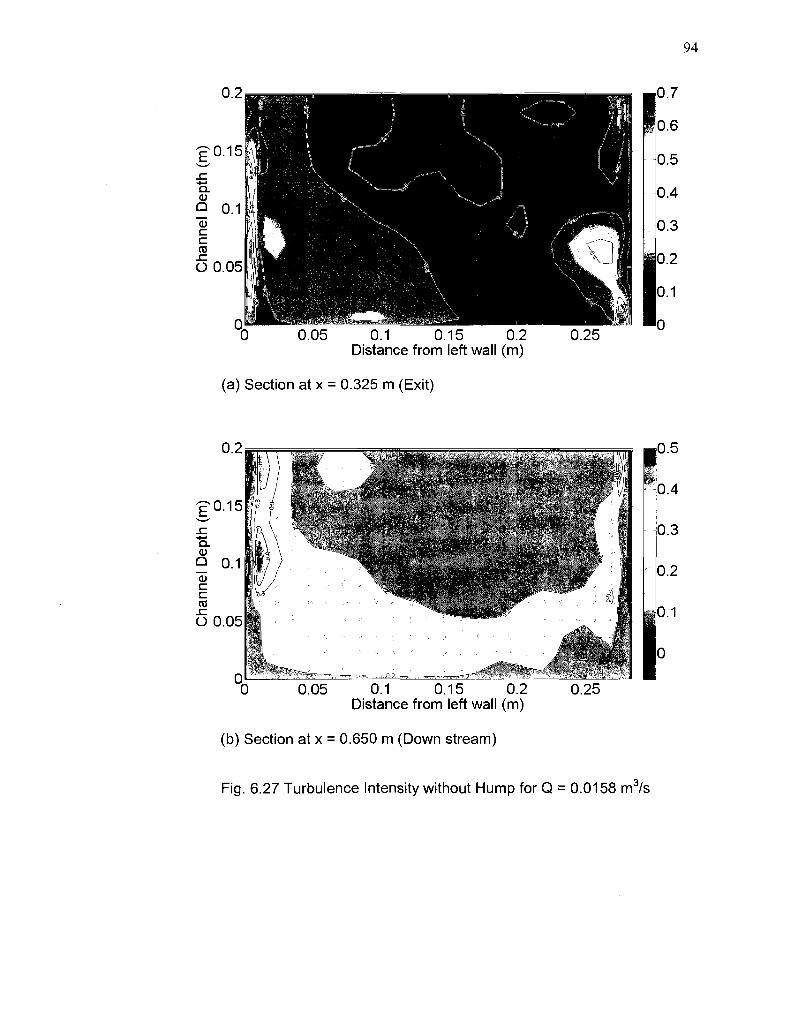
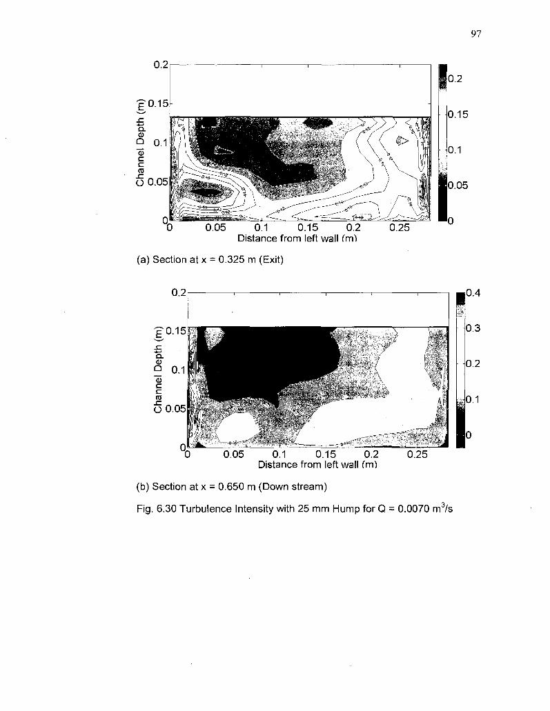
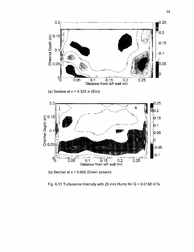
6.1.7 Turbulence intensity diagrams 58

ix

6.2.0 Numerical simulation 60

6.2.1 Turbulence model 61

6.2.2 Boundary conditions 61

6.2.3 Solution procedure 61

6.2.4 Discussion of results 62

6.2.5 Velocity distribution data for the case of no hump 62

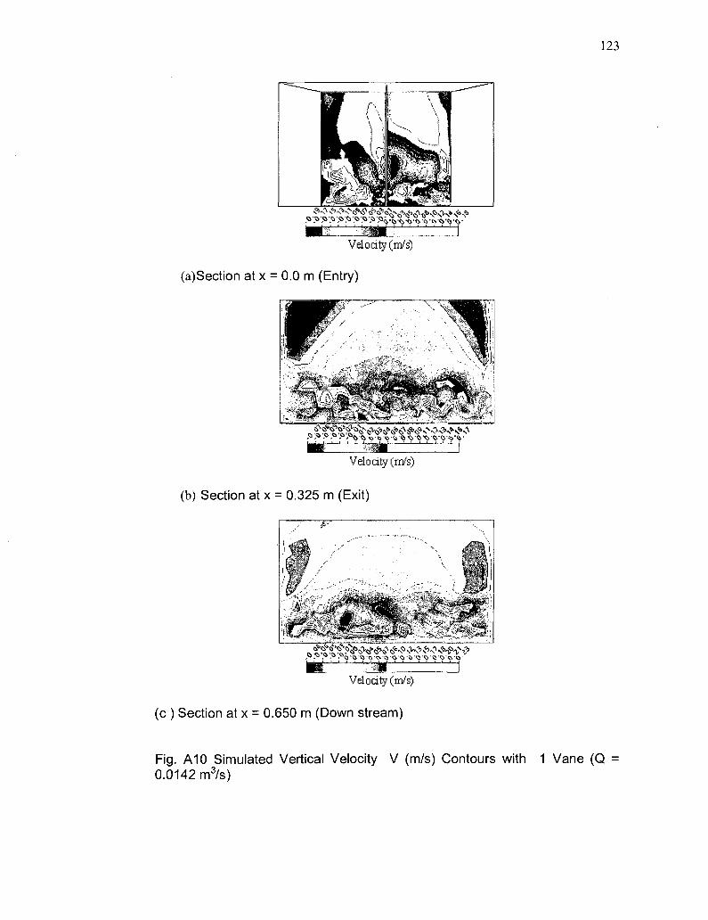
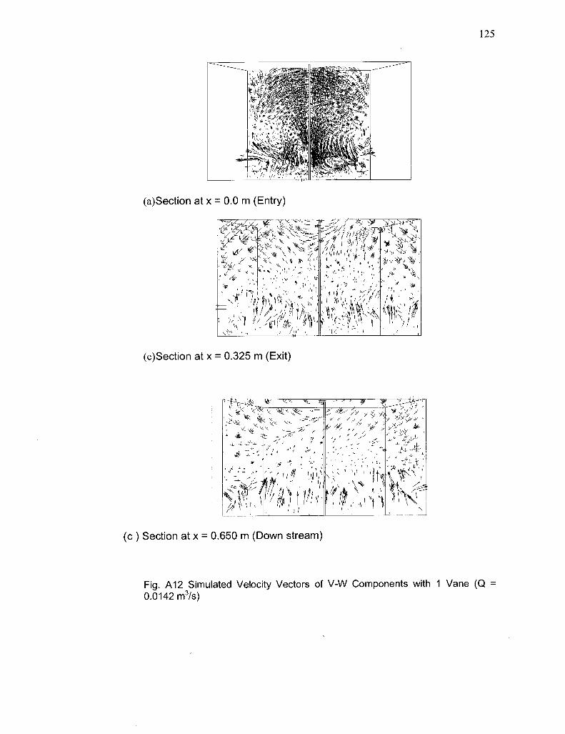
6.2.6 Velocity distribution for the case of a single vane splitter 63

6.2.7 Velocity distribution for the case of 3-vane splitter 64

6.2.8 Boundary shear stress 64

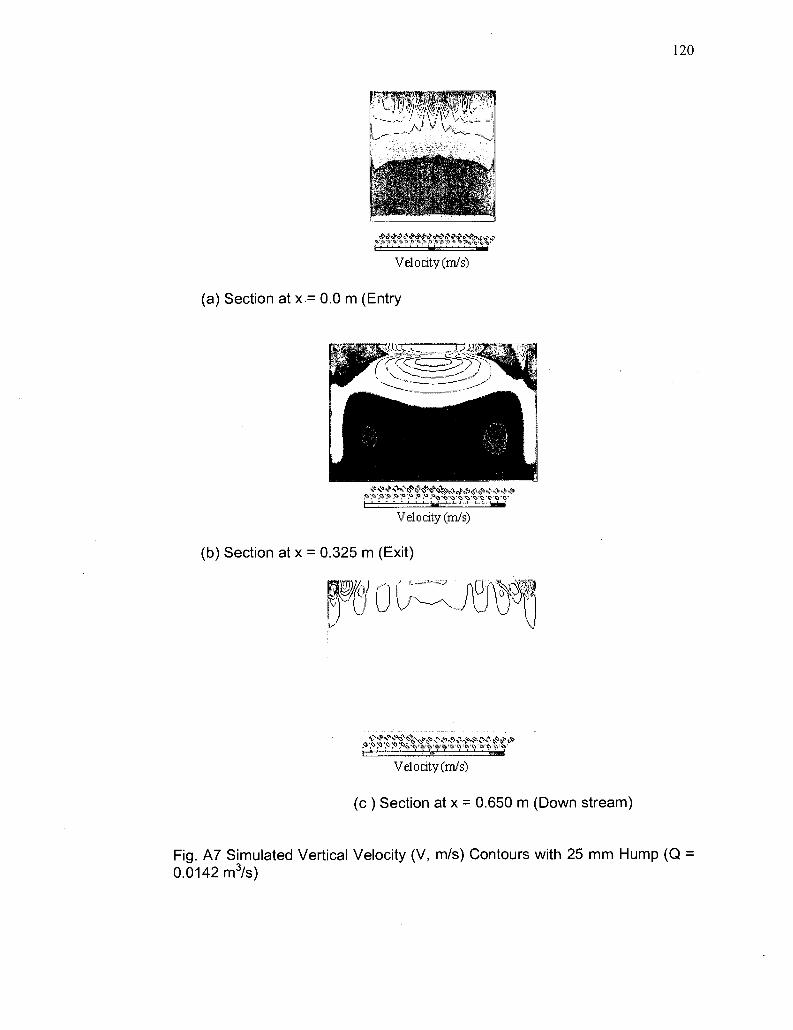
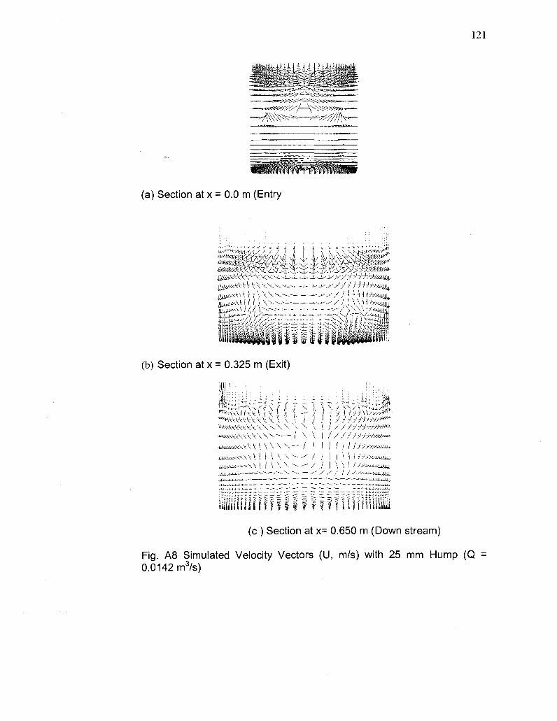
6.2.9 Velocity Distribution for the case of 25 mm hump 65

CHAPTER 7 CONCLUSIONS AND RECOMMENDATIONS 66

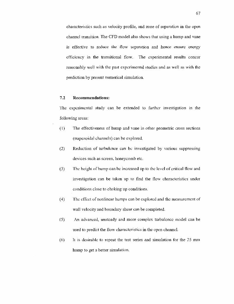
7.1 Conclusions 66

7.2 Recommendations 67

REFERENCES 109

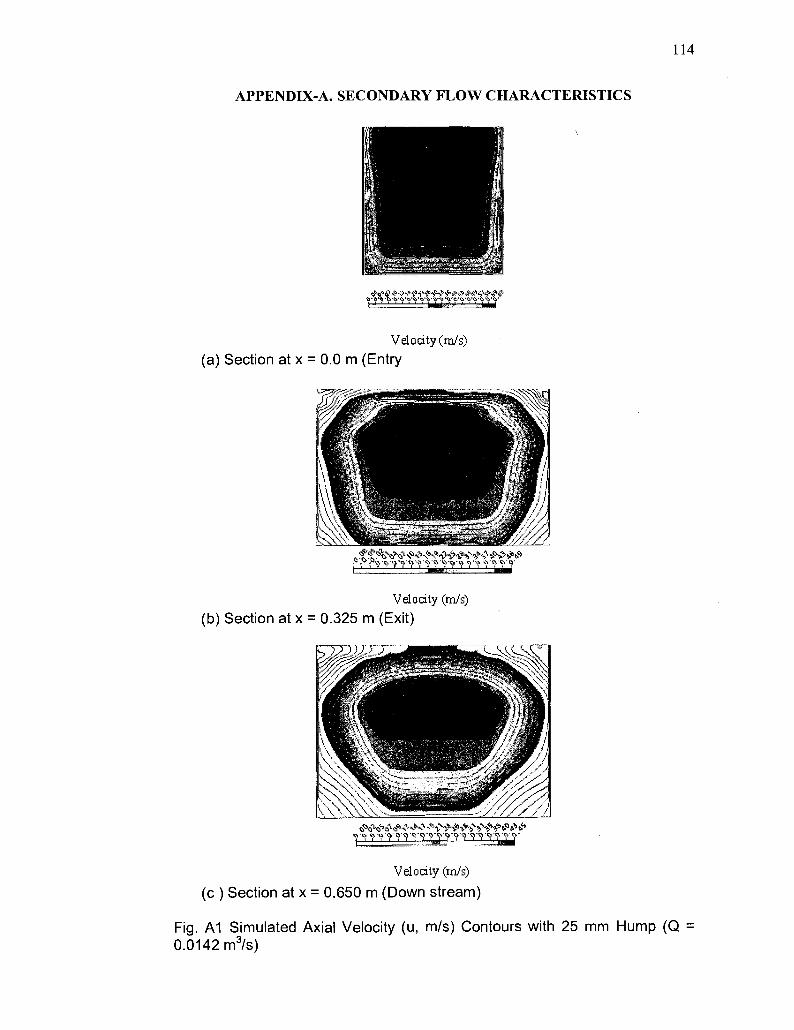
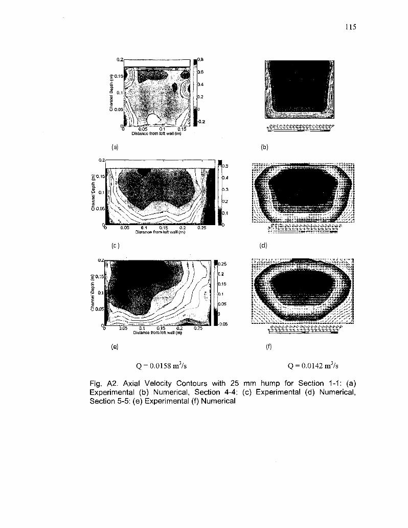
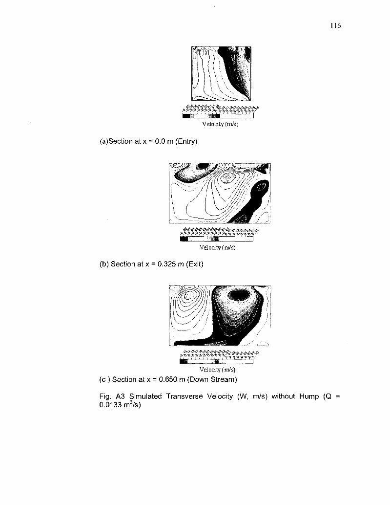
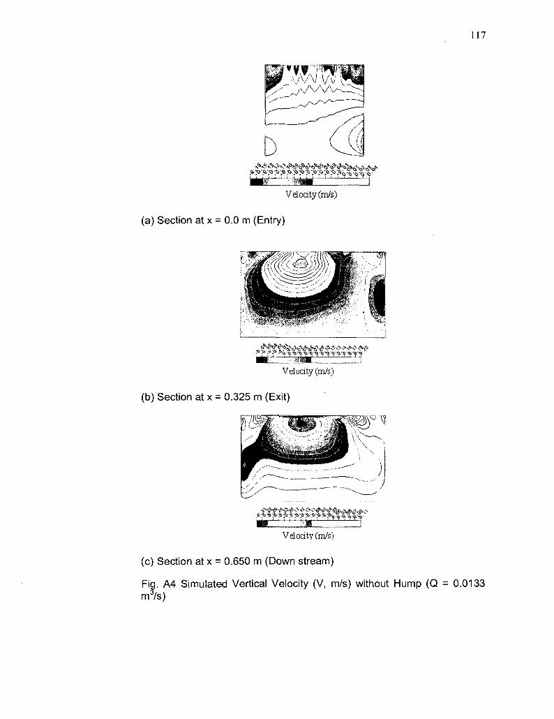
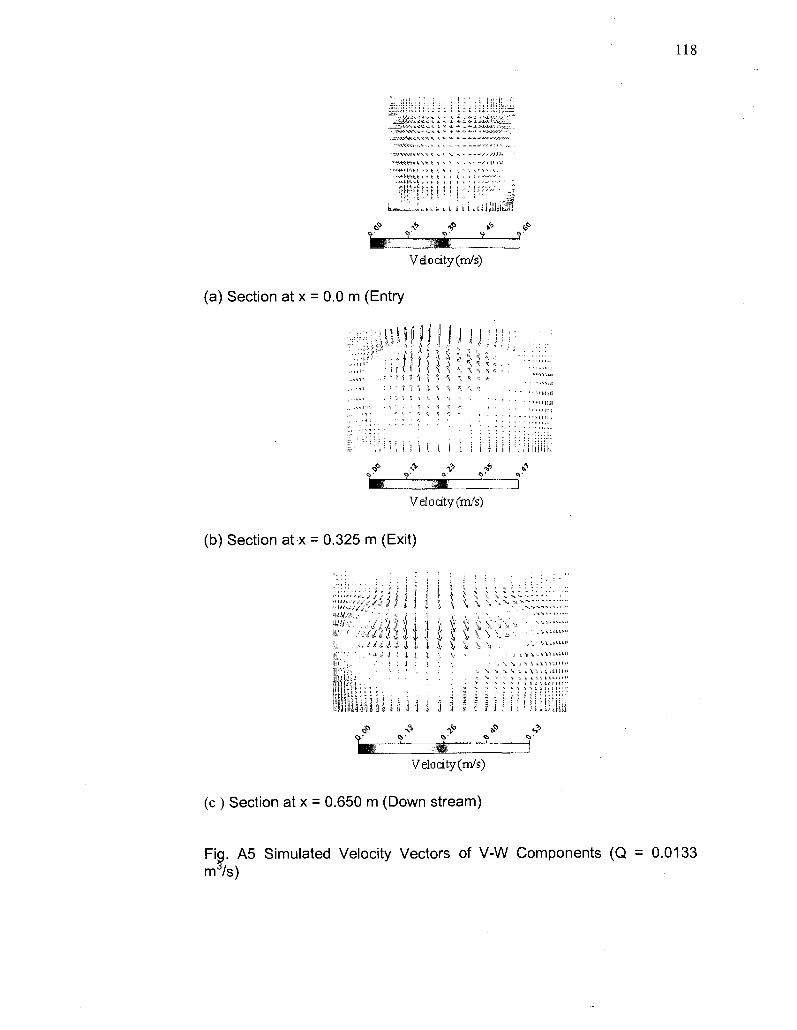
APPENDIX-A Secondary flow characteristics 114

X

LIST OF FIGURES

Fig. 1.1 Plan of open channel expansions 4

Fig: 2.1. Boundary-layer flow showing the separation point S

(Schlichting, 2000) 5

Fig 2.2 Stagnation Point Flow, after H. Fottinger (1933), (a) Free Stagnation-point

flow without separation, (b) Retarded stagnation-point flow, with separation

(Schlichting, 2000) 6

Fig 3.1 Plan of open channel transition with elevation of two humps 27

Fig 3.2 Open channel transition with 3 vanes 28

Fig 4.1 Specific energy diagram for a transition 35

Fig. 6.0.1 The computational domain for simulation 62

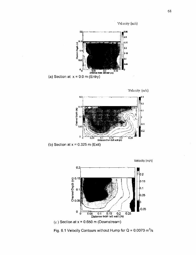
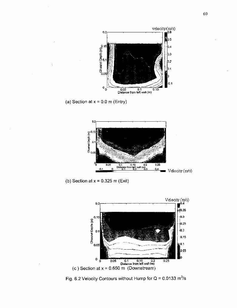
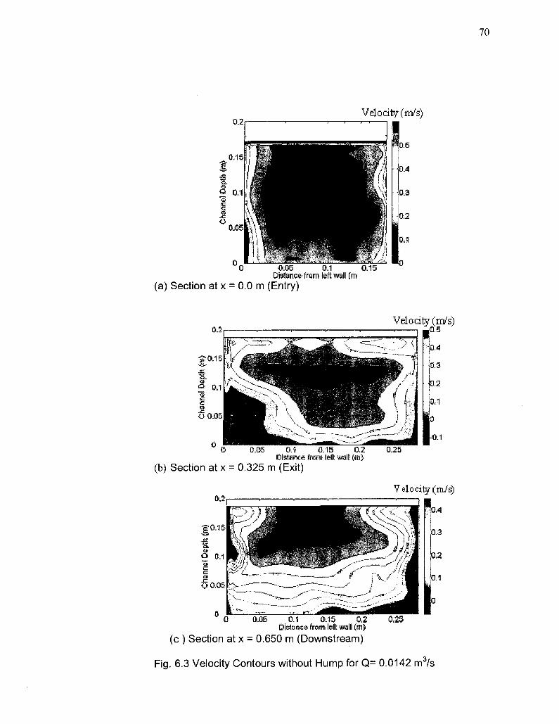
Fig.6.1 -6.15 Velocity contours and velocity distribution 68

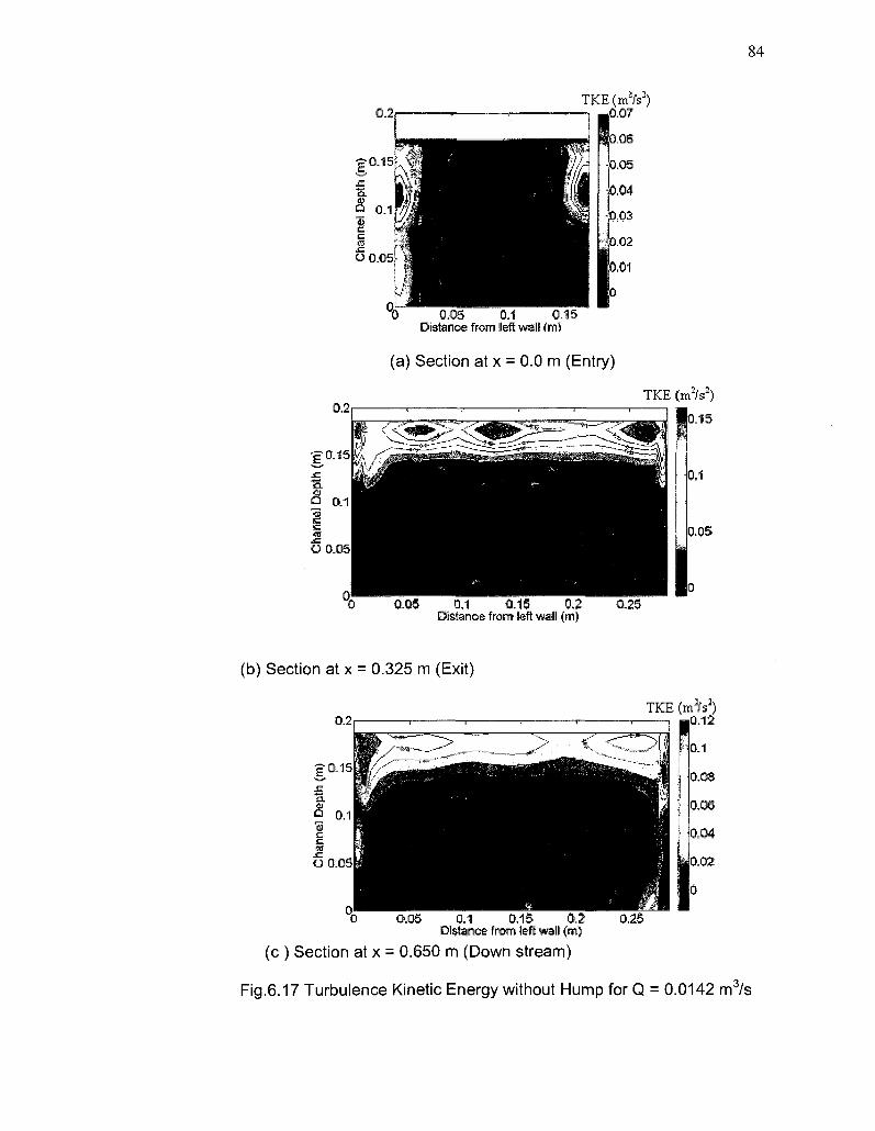
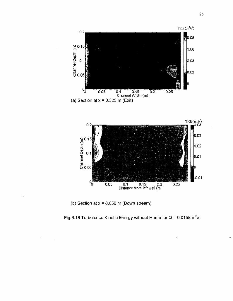
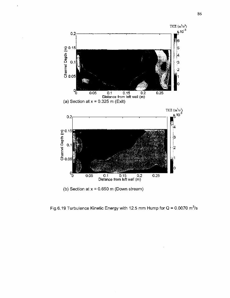
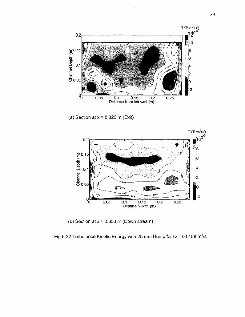
Fig. 6.16-6.24 Turbulence kinetic energy 83

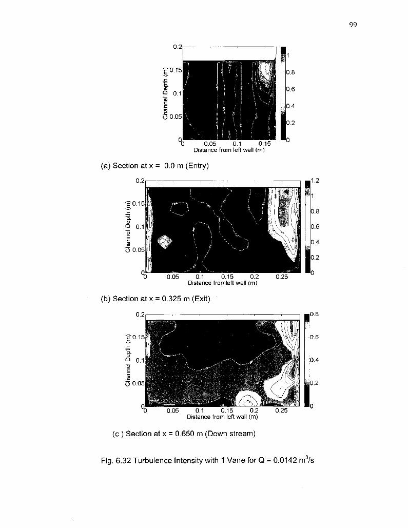
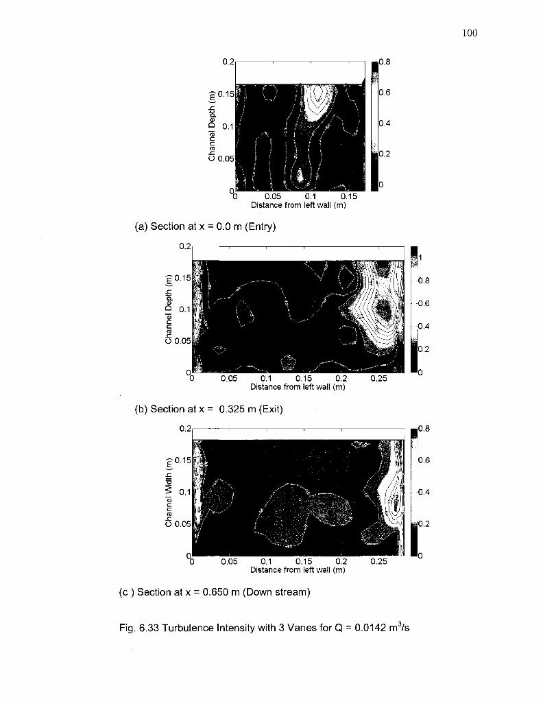
Fig. 6.25-6.33 Turbulence intensity 92

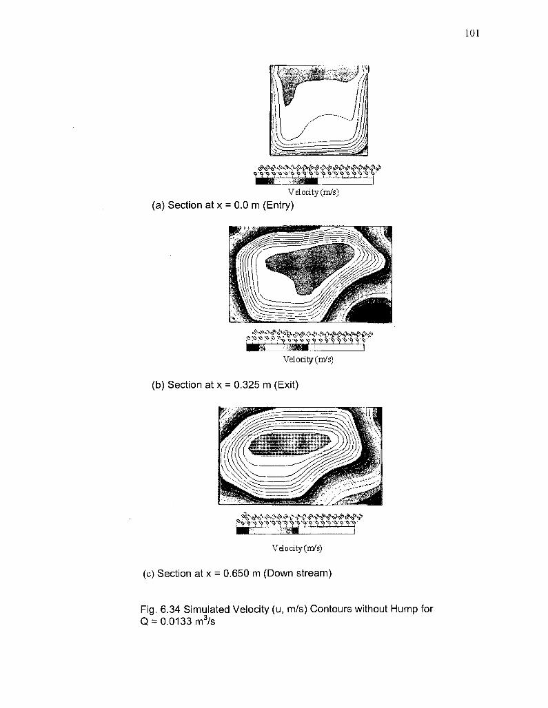
Fig. 6.34 Simulation without Hump/Vane 101

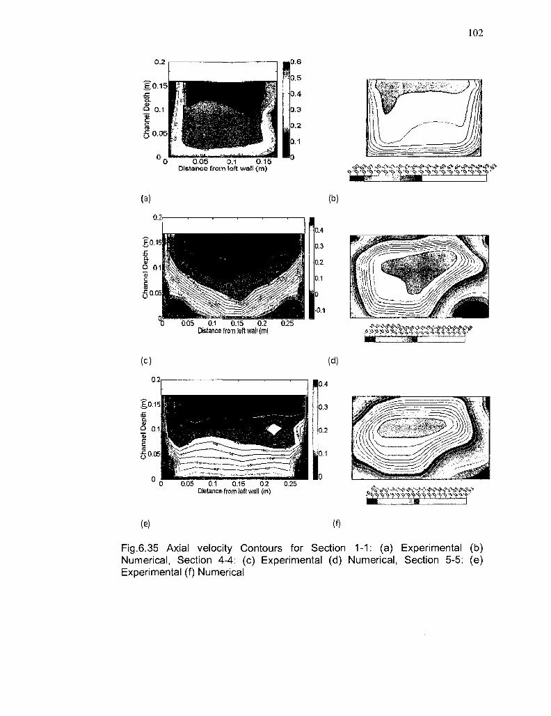
Fig.6.35 Axial velocity contours without hump for Section 1-1:

(a) Experimental (b) Numerical, Section 4-4: (c) Experimental

(d) Numerical, Section 5-5: (e) Experimental (f) Numerical 102

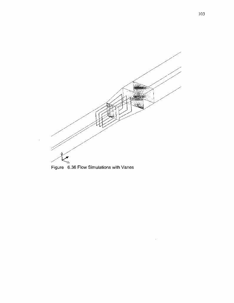
Fig. 6.36 Flow simulation with vanes 103

Fig. 6.37 Flow simulation with 1 vane 104

Fig.6.38 Axial Velocity Contours with 1 Vane

for Section 1-1: (a) Experimental (b) Numerical,

Section 4-4: (c) Experimental (d) Numerical,

xi

Section 5-5: (e) Experimental (f) Numerical 105

Fig. 6.39 Simulation with 3 vanes 106

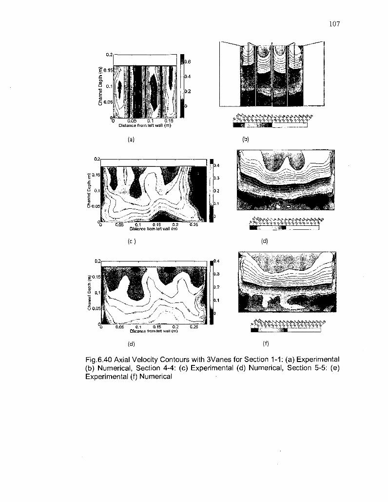
Fig.6.40 Axial Velocity Contours with 3Vanes

for Section 1-1: (a) Experimental (b) Numerical,

Section 4-4: (c) Experimental (d) Numerical,

Section 5-5: (e) Experimental (f) Numerical 107

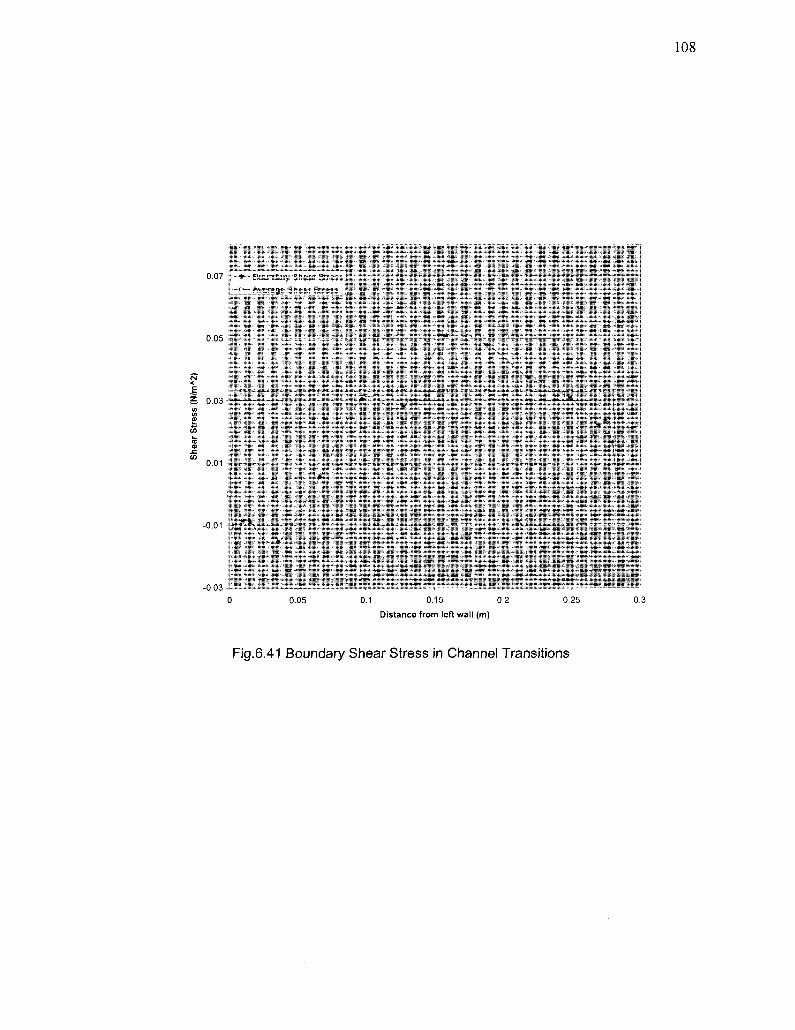
Fig. 6.41 Boundary shear stress 108

xii

LIST OF TABLES

Table 2.1 Efficient angle of divergence 14

Table 2.2 Loss co-efficient for different transitions 22

Table 2.3 Summary of separation methods in channel expansions 23

Table 2.4 Flow regimes in separation process 25

Table 6.1 Flow characteristics of laboratory experiments 52

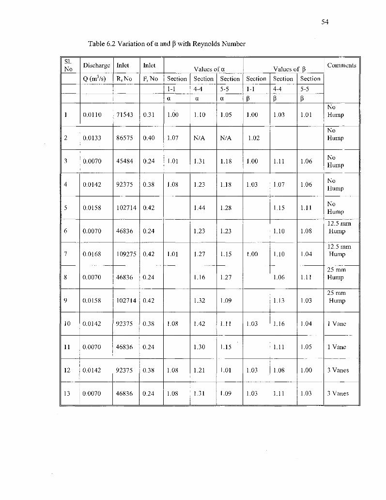
Table 6.2 Variation of a and (3 with Reynolds Number 54

Table 6.3 Variation of % of area of reverse flow field

with inlet Reynolds number 55

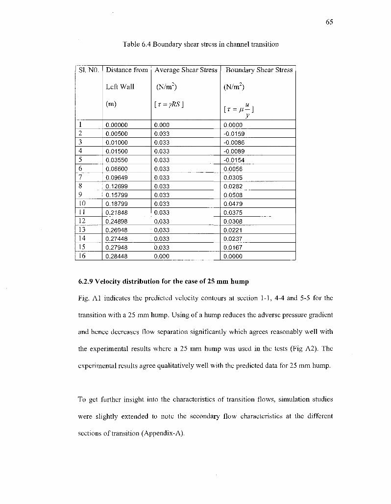
Table 6.4 Table 6.4 Boundary shear stress in channel transition 65

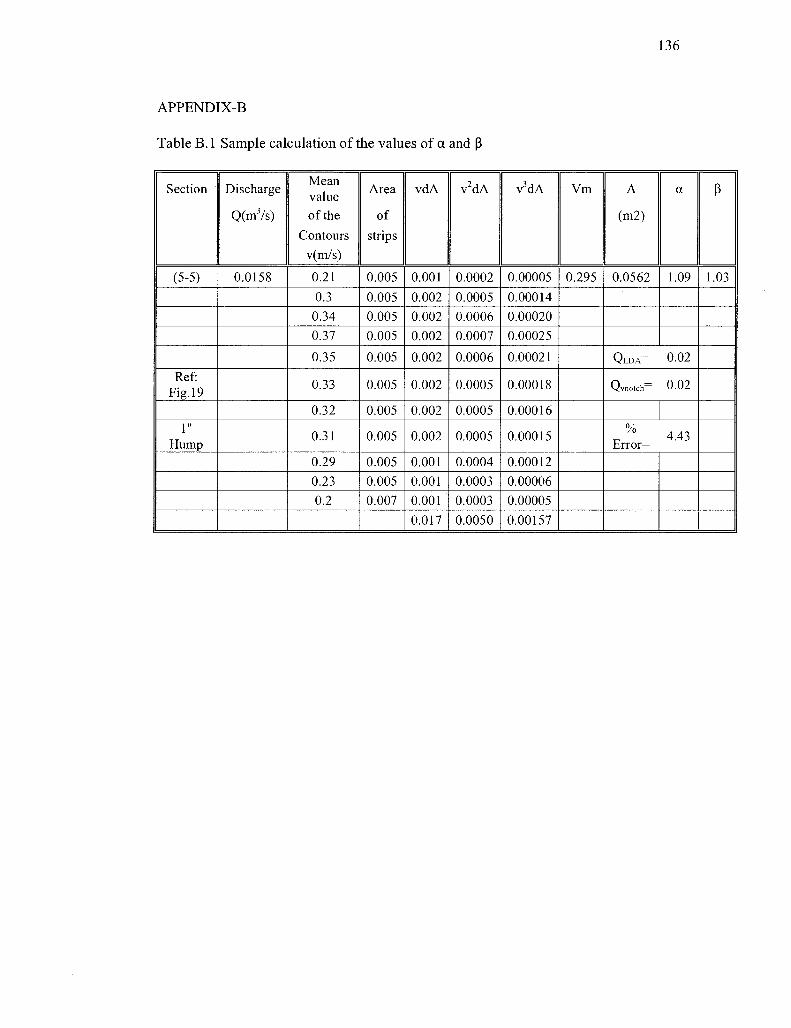
Table B.l Sample calculation of the values of a and p 136

LIST OF SYMBOLS

a = Velocity co-efficient

P = Momentum co-efficient

y = Specific gravity of water

5 = Boundary layer thickness

s = Rate of energy dissipation

co = Specific rate of dissipation

u. = Molecular viscosity

v = Kinematic viscosity

p = Density of water

K = Total kinetic energy

k = Turbulent kinetic energy

x = Shear stress

0 = Angle of Transition

u, v, w = Velocity components in x, y, z direction

p = Pressure

q = Discharge per unit width

E = Total energy

H = Total head

Em = Mean kinetic energy of flow

R = Hydraulic radius

U = Average velocity

V = Maximum observed velocity

XIV

Vm=Weighted mean velocity

AP=Change in pressure between two points

AA = Elementary area of flow corresponding to velocity v

1

Chapter 1

Introduction

1.1 General remarks

Flow separation in open channel expansion has been identified as one of the major

problems encountered in many hydraulic structures such as irrigation networks,

bridges, flumes, aqueducts, power tunnels and siphons. In most of these cases, the

flows are generally subcritical in nature. In such expansions, the divergent flow can

lead to a continuous reduction of kinetic energy and its conversion in part to pressure

energy. During this process, some energy is lost due to changing flow condition in the

channel expansion. Moreover, the presence of adverse pressure gradient causes flow

separation due to the inability of flow to adhere to the boundaries and subsequent

formation of eddies resulting significant head losses. In such cases control of flow

separation is required to reduce bed and bank erosion. Moreover, minimizing the head

loss in irrigation canals increases the command area served by them. In the past,

efforts have been made to design efficient transition walls to avoid flow separation.

Secondary measures have also been taken to control flow separation by the aid of

splitter walls (vanes), baffles, humps etc to supplement primary measures. Despite

extensive theoretical and experimental investigations on expansions in close conduits,

the research on open channel expansions has comparatively been less in number and

more in terms of one dimensional analysis. Therefore, it is desirable in hydraulic

engineering to investigate structures of open channel expansions to evaluate the

velocity distribution, boundary shear distribution, to control flow separation, and to

design hydraulic structures properly. These measures are also needed to assist the

2

problems encountered in sediment transport, wastewater and pollutant transport

phenomena.

Earlier investigators (Chaturvedi 1963, Smith 1966, Soliman 1966, Kline 1962, Feil

1962, Daugherty 1962) have carried out a few studies in this field and suggested

various methods to suppress flow separation. Although their initial contributions are

laudable, yet most of the studies on expansion are limited to one dimensional flow

and lack quantitative data. This is especially true for the case when vanes are used to

reduce separation in transitions. Recent flow measurements techniques and digital

technology like Laser Doppler Anemometry (LDA) have created new opportunity to

investigate complex flow characteristics of open channel expansion and broaden our

present level of knowledge on these areas which may help to provide new engineering

design inputs when field conditions are encountered.

1.2 Objective of the study

The objectives of the study are enumerated below:

1. To determine mainly the mean velocity profile of subcritical flows in

rectangular open channel transitions, and to determine the boundary shear

stress of the channel bed. The latter is limited to a few select cases.

2. To determine the effects of hump in reducing flow separation and its

adverse effects, to investigate the effect of splitter vanes to reduce or

remove flow separation and in turn to reduce energy losses.

3. To collect limited turbulence data using Laser Doppler Anemometer

(LDA) for possible later model validation.

3

4. To conduct a few numerical simulations as an alternative to experiment

and to compare the predicted numerical simulation data with the

experimental data.

1.3 Scope of the study

The present study is mainly experimental supplemented by a few numerical

simulations. The analysis was performed using the current data collected as well as

the available existing data. To this end, a Plexiglas rectangular laboratory model was

constructed to facilitate data collection by the Laser Doppler Anemometer (LDA).

Flow separation was visualized using dye techniques in some cases.

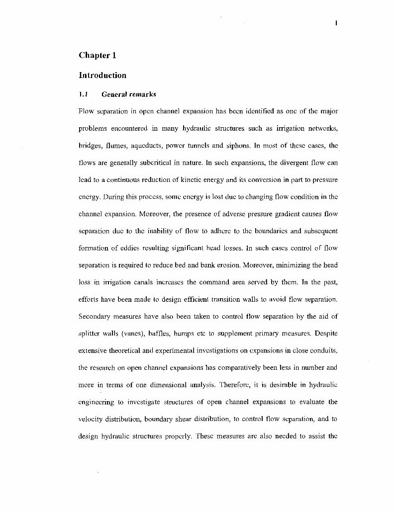
A 325 mm long transition with 19.78 divergent angles was connected with a 171 mm

wide straight upstream and 284.5 mm wide down stream horizontal rectangular open

channels (Fig. 1.1).

Two humps of 12.5 mm and 25 mm were formed by raising the bed level in the

expanding section. They were installed to see the effects of hump as a flow separation

control device.

Two sets of split vanes, one with a single vane and the other with three vanes in the

transition were used to study the effect of vanes in reducing the separation and to

collect quantitative data for turbulent characterization.

An inclined (1:5) manometer was mounted to get pressure reading at different height

of the transitional section of the channel. It could read the water level to the nearest

mm

The ranges of parameters (Froude's numbers, Reynolds numbers, velocity and

discharge) were varied during the tests.

A limited number of CFD numerical simulations were also conducted. These included

the use of devices such as humps and splitter vanes that were placed in the transition.

The predictions of simulation were compared with the test data.

:EEEE

Upstream Channel

=i /<ff W

Hi

Transition

zBH

Down Stream Channel

Fig. 1.1 Plan of open channel expansion

5

CHAPTER 2

LITERATURE REVIEW

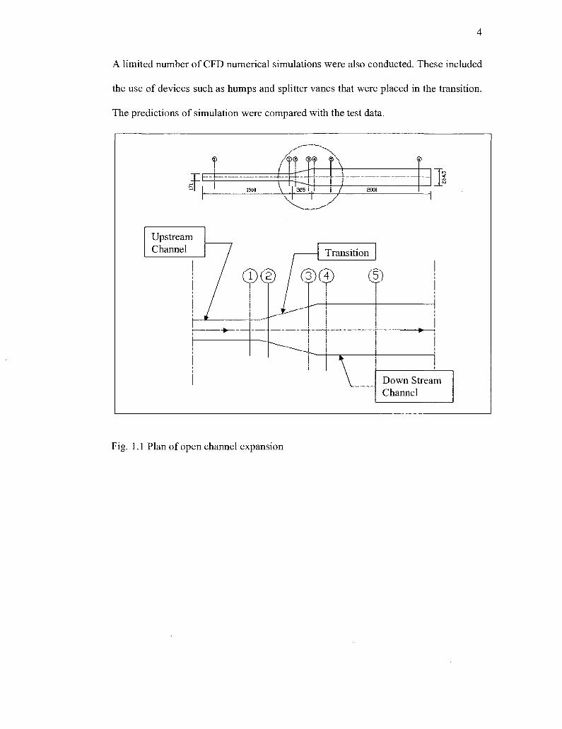
2.1 Flow separation mechanism

Flow separation occurs when the velocity at the stationary wall is zero or negative,

and an inflection point exists in the velocity profile. Moreover, a positive or adverse

pressure gradient occurs in the direction of flow. Channel expansion or contraction,

sharp corners, turns and high angles all represent decelerating flow situations where

the fluid in the boundary layer losses its kinetic energy leading to separation. The

flow separation of a boundary layer is depicted in the Fig. (2.1). The position of the

separation can be given by the condition that the velocity gradient perpendicular to

the wall vanishes at the wall, i.e. the wall shear stress rw vanishes (Schlichting, 2000):

TW=M

fdu"

v ^ y w

= 0 (Separation) (2.1)

The point of separation can be determined by solving boundary layer differential

equations.

--V4 »""_ . < - ' »***

'/

J.A-.. S

y

-> u

Fig: 2.1. Boundary-layer flow showing the separation point S (Schlichting, 2000)

6

Flow separation accompanying an expansion in an open channel results in the

increase of depth in the expansion and flow separates from the walls. Fig. 2.2a shows

the flow against a normal wall. There is an adverse pressure gradient in the direction

of flow due to the presence of a symmetrical central streamline. However, there is no

flow separation. In the fig.2.2b shows the condition in which a boundary layer with

adverse pressure gradient exists due to the presence of a very thin splitter plate placed

at right angles to the wall. Hence, the boundary layer formed along the splitter plate

separates from the splitter plate. Thus, flow separation is extremely sensitive to small

changes in the shape of the body. Flow separation in subcritical steady flow occurs in

decelerated flow i.e., when— > 0. It also occurs when there is an abrupt change in dx

the wall alignment.

Fig 2.2 Stagnation Point Flow, after H. Fottinger (1933), (a) Free Stagnation-point

flow without separation, (b) Retarded stagnation-point flow, with separation

(Schlichting, 2000)

7

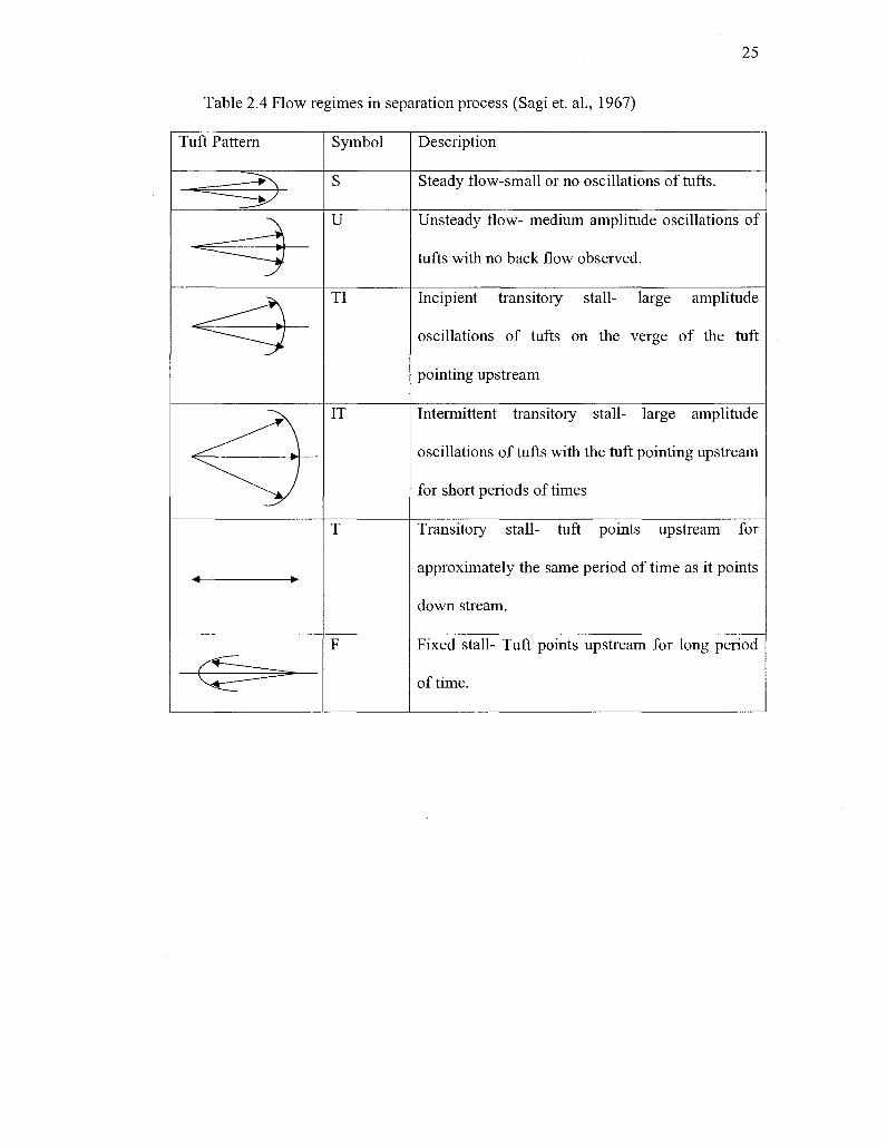
Carlson, Johnston and Sagi (1967) used tufts to trace flow separation. They divided

the flow into six categories according to the relative position of the tufts with the

flow. (Table2.4)

The first attempts at describing separated flow past blunt bodies are due to Helmholtz

and Kirchhoff in the framework of the classical theory of inviscid fluid flows. There

was no adequate explanation as to why separation occurs. Prandtl (1904) was the first

to recognize the physical cause of separation at high Reynolds numbers as being

associated with the separation of boundary layers that must form on all solid surfaces.

Flow development in the boundary layer depends on the pressure distribution along

the wall. If the pressure gradient is favorable, i.e. the pressure decreases downstream,

then the boundary layer remains well attached to the wall. However with adverse

pressure gradient, when the pressure starts to rise in the direction of the flow, the

boundary layer tends to separate from the body surface.

2.2 Boundary layer flow

A boundary layer consists of a thin region adjacent to solid surfaces and a substantial

region of inertia-dominated flow far away from the wall. The flow very close to the

wall (viscous sub-layer) is influenced by viscous effects and does not depend on free

stream parameters. The mean flow velocity depends on the distance y from the wall,

fluid density p and viscosity ju and the wall shear stress TW .

Therefore,

\J=fy,p,M,rJ (2.2)

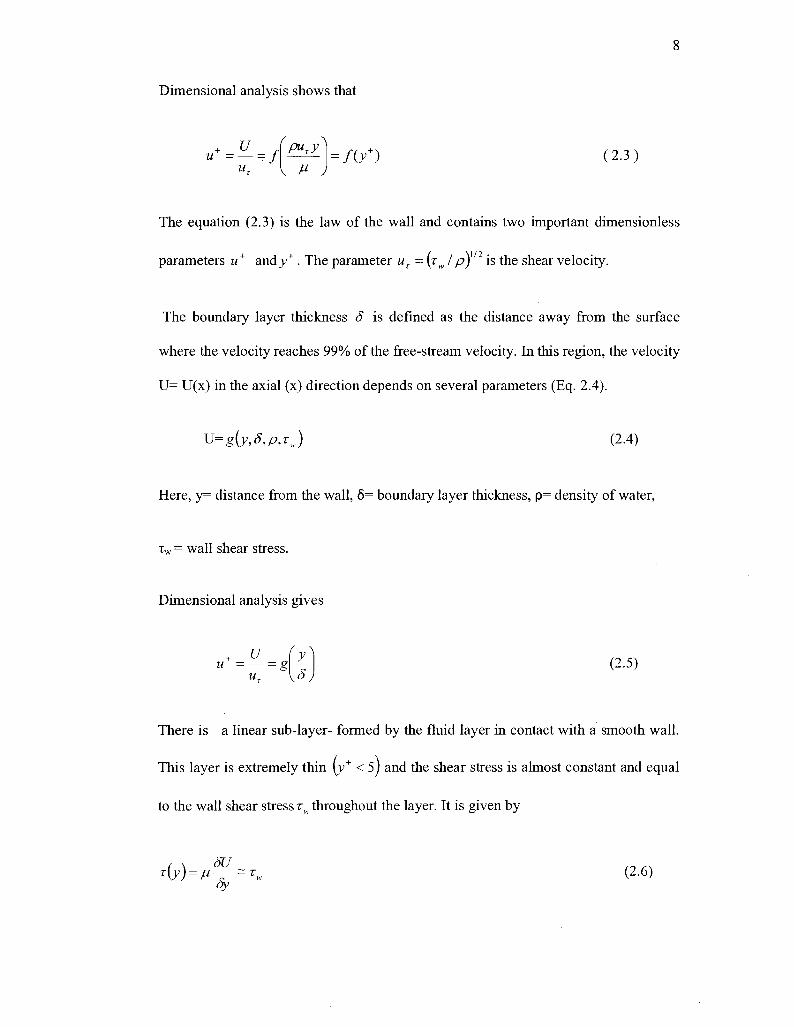
Dimensional analysis shows that

+ U f( u = — = / ^ = f(y+) (2.3)

The equation (2.3) is the law of the wall and contains two important dimensionless

parameters u+ andy+ . The parameter uT = (rw I pf is the shear velocity.

The boundary layer thickness 8 is defined as the distance away from the surface

where the velocity reaches 99% of the free-stream velocity. In this region, the velocity

U= U(x) in the axial (x) direction depends on several parameters (Eq. 2.4).

XJ=g(y,S,p,Tw) (2.4)

Here, y= distance from the wall, 6= boundary layer thickness, p= density of water,

TW = wall shear stress.

Dimensional analysis gives

+ U u = — = g ry^ (2.5) \u J

There is a linear sub-layer- formed by the fluid layer in contact with a smooth wall.

This layer is extremely thin (y+ < 5) and the shear stress is almost constant and equal

to the wall shear stress rM, throughout the layer. It is given by

r(y) = ^ = rw (2.6) Sy

9

Integrating with respect to y and applying boundary condition U=0 if y=0, a linear

relationship between the mean velocity and the distance from the wall is established.

T V U = ^ - (2.7)

There is a region outside the viscous sub-layer (30 <y+ <500) where viscous and

turbulent effects are both important. The shear stress r varies slowly with distance

from the wall and within this inner region it is assumed to be constant and equal to the

wall shear stress. In this region there is a dimensionally correct form of the functional

relationship between u+ and y

M+ = - l n ^ + + 5 = - ln(^y + ) (2.8)

k k

Here, k=0.4, B=5.5, (or E=9.8) for smooth wall. Because of the logarithmic

relationship between u+ and y+, the above formula is called the log-law and the layer

where y+ takes the values between 30 and 500, the log-law layer.

2.3 Losses in open channel transitions

A channel transition may be defined as a change in the direction, slope, or cross

section of the channel that brings a change in the flow condition .Though all

transitions of engineering interest are relatively short features, yet they may affect the

flow for a great distance upstream and downstream (Henderson, 1966). Again, the

design and performance of transitions are critically dependent on sub-critical and

super critical flow regimes. The calculation of energy losses and determination of the

transition profile to provide a good velocity distribution at the end of the transition,

are two problems areas that need the attention of hydraulic engineers.

10

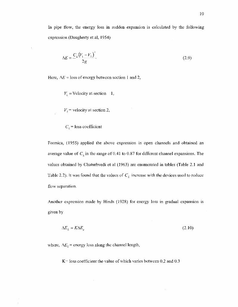
In pipe flow, the energy loss in sudden expansion is calculated by the following

expression (Daugherty et al, 1954)

AE = C ^ ~ V ^ (2.9) 2g

Here, AE = loss of energy between section 1 and 2,

Vx = Velocity at section 1,

V2 = velocity at section 2,

CL = loss coefficient

Formica, (1955) applied the above expression in open channels and obtained an

average value of CLin the range of 0.41 to 0.87 for different channel expansions. The

values obtained by Charurbvedi et al (1963) are enumerated in tables (Table 2.1 and

Table 2.2). It was found that the values of CL increase with the devices used to reduce

flow separation.

Another expression made by Hinds (1928) for energy loss in gradual expansion is

given by

AEL=KAEu (2.10)

where, AEL = energy loss along the channel length,

K= loss coefficient the value of which varies between 0,2 and 0.3

11

AEU = the change in velocity heads between the two sections under

considerations, viz. 2g 2g

Formica (1955) presented experimental data showing energy losses in sudden

expansions some 10 % less than those given by Eq. (2.9). Experiments were carried

out by Mishra (1977) where depth hi, I12,113 were not very different from one another.

The energy loss in his experiments with B1/B2 ranging from 1.33 to 2.0 was 1.6 to 4.0

times that given by Eq. (2.9). Thus the energy loss in the case of an abrupt flow does

not agree well with the theory of closed conduit flow.

A special feature of the flow in an expansion connecting rectangular conduits of

widths Bi and B2 is found to be the lack of symmetry when the expansion ratio is

large. Abbott et al. (1962) studied diffuser flows and found that the length of the eddy

on both walls is the same as long as B1/B2 < 1.5 but at larger values of BI/B2, the

eddy on one side becomes larger than on the other and the centre line of the channel

no longer remains the line of maximum velocity. The eddy lengths are independent of

Reynolds number Re and are dependent on Bi/B2.

Millsaps et al. (1953) investigated flow in an open channel expansion and plotted a

series of velocity profiles for different Reynolds numbers. The results show that when

the Reynolds number is large, the velocity is positive over the entire cross section and

at lower Reynolds numbers; reverse flows are observed near the walls denoting flow

separation. Hamel (1916) found that for larger angles of divergence, flow separation

occurs earlier, at lower Reynolds numbers.

12

The divergent angle plays an important role in flow separation. When the divergence

angle 0 is small flow through expansions can be non-uniform but not necessarily very

unsteady. The transitional flow is sometimes theoretically called irrotational. This is

because of non uniform pressure distribution and high degrees of eddying due to flow

separation. The pressure distribution may not be truly hydrostatic because of

transverse and vertical velocity components.

Chaturvedi (1963) found that when the curvature of divergence is high, the

domination of local stresses will prevail due to pressure variation and lateral inertial

forces.

2.4 Turbulence characteristics in channel transition

Open channel flows are regularly turbulent in nature. Turbulent fluid flow is an

irregular condition of flow characterized by diffusivity, large Reynolds number, 3D-

vorticity fluctuations, dissipations, and continuum in nature. Turbulence is better

described by its eddy motion. It consists of a continuous spectrum of largest to

smallest eddies having swirling motion generating kinetic and dissipating to thermal

energy. Turbulence represents the "cascade process" that occurs in the atmosphere. In

another words, energy associated with large-scale motion generates larger eddies. The

larger eddies transfer this energy to smaller ones and these smaller scales eddies then

transfer the energy to the next smallest eddies. Eventually, the energy is dissipated

into heat through molecular viscosity. In the study of turbulence, the generation and

dissipation of turbulent kinetic energy are very important phenomena.

General hydraulic and transport model assumes that flows in open channels are

uniform and unidirectional (Papanicolaou et al. 2001). Despite few successes, those

models may under predict or over predict sediment transport, scouring in the natural

channel due to the presence of secondary flows ( MaLelland et al. 1999). Prandlt

13

(1955) identified two types of secondary flows such as (i) skew-induced secondary

flow called secondary flows of Parndlt's first kind and (ii) stress induced secondary

flow or secondary flows of Prandalt's second kind due to anisotropy of turbulent

fluctuations. The stress induced secondary flows are generated du to the channel

transitions and bed undulations. Though several studies were conducted on secondary

flows on meandering channel and bed form, very few studies were carried out on

turbulent flow characteristics in channel transitions. Sukhodolov et al. 1998). Mehta

(1981) and El—Shewey and Joshi (1996) investigated the effects of a sudden channel

expansion on turbulence characteristics over smooth surfaces. They found that the

high intensity turbulence occurs either close to the surface or near the bed because of

the Prandalt's second kind secondary flows developed at the channel transitions.

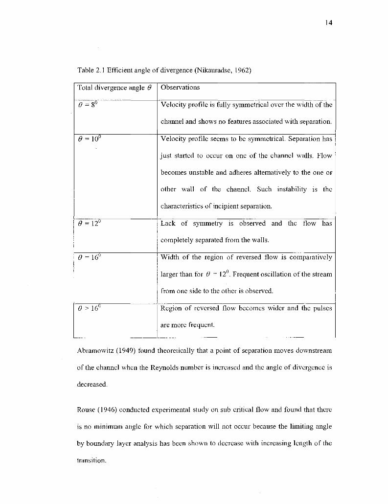
2.5 Geometry of divergence to control flow separation

Nikauradse (1962) conducted experiments to determine an efficient angle of

divergence to see the separation characteristics of flow. The observations reported by

him are given in Table 2.1.

14

Table 2.1 Efficient angle of divergence (Nikauradse, 1962)

Total divergence angle 9

9=8°

6> = 10°

e = 12°

# = 16°

9 >16°

Observations

Velocity profile is fully symmetrical over the width of the

channel and shows no features associated with separation.

Velocity profile seems to be symmetrical. Separation has

just started to occur on one of the channel walls. Flow

becomes unstable and adheres alternatively to the one or

other wall of the channel. Such instability is the

characteristics of incipient separation.

Lack of symmetry is observed and the flow has

completely separated from the walls.

Width of the region of reversed flow is comparatively

larger than for 9 = 12°. Frequent oscillation of the stream

from one side to the other is observed.

Region of reversed flow becomes wider and the pulses

are more frequent.

Abramowitz (1949) found theoretically that a point of separation moves downstream

of the channel when the Reynolds number is increased and the angle of divergence is

decreased.

Rouse (1946) conducted experimental study on sub critical flow and found that there

is no minimum angle for which separation will not occur because the limiting angle

by boundary layer analysis has been shown to decrease with increasing length of the

transition.

15

Smith et al.(1966) have found that the total divergence angle 9 should not be more

than 11 16 to avoid flow separation. Separation occurs when the total divergence

angle is increased to > 19 (except for B1/B2 < 1 to 2).

2.6 Design considerations for transitions

Different aspects of designing transitions investigated by different researchers are

enumerated below:

The distribution of mean velocity at the inlet to the expansion influences the energy

lost in the expansion and the efficiency of the system. High ratios of centre velocity to

mean velocity in the cross section give poor efficiencies and high energy loss. When

there is adequate and proper lateral distribution of momentum, there will be no flow

separation at all (Chaturvedi, 1963).

A uniform velocity at the exit is more desirable to minimize energy loss as a uniform

velocity distribution produces lower exit velocity for a given flow rate and lowest rate

of momentum out flow and thus maximizes pressure rise and minimize exit losses

(Waitman et al. 1961). Efficient conversion of kinetic energy to pressure energy plays

an important role for an efficient transition design (Chaturvedi, 1963). Gradual

expansion can minimize the adverse pressure gradient. Hence the probability of

separation is reduced when the pressure gradient — is lower as the angle of dx

divergence is smaller (Chaturvvedi, 1963)

16

2.7 Method of control of flow separation

The loss of momentum or energy due to flow separation is detrimental for a diffuser

or channel transition. Probable solutions may be the prevention of the initial

occurrence, early elimination, or some reduction. Prevention or reduction of

separation has little difference. They essentially differ only in the degree of control

required. Control techniques are broadly classified as (a) devices without auxiliary

power and (b) auxiliary powered devices. The flow separation from a continuous

surface is governed by two factors, adverse pressure gradient and viscosity. In order

to remain attached to the surface, the flow must have sufficient energy to overcome

the adverse pressure gradient, the viscous dissipation along the flow path, and the

energy loss due to the change in momentum. This loss has a significant effect on the

channel walls where momentum and energy are much less than in the outer part of the

boundary layer. If the loss of energy is so much that the fluid cannot move ahead, then

the flow separates from the wall. On the contrary, if the momentum and energy

adjacent to walls are sufficient, then no separation occurs. Hence, techniques for

controlling flow separation are either (a) to design the body surface configuration in

such a way that a sufficiently high energy level is maintained along the flow path near

the walls or (b) to boost the energy level by a physical device placed at a suitable

position along the flow path (Chang, 1976).

The dilemma is to maintain sufficient energy level of the fluid along the flow path to

overcome the pressure rise and viscous friction in the boundary layer. In the past,

various methods have been adopted to achieve this condition. These are as follows:

17

(a) Elimination of viscosity effect by suction of boundary layer: Suction removes

the deceleration of flow particles in the neighborhood of the wall and hence

prevents flow separation.

(b) The increasing momentum of the surface fluid: The mixing of shear layer

particles can be increased by using an auxiliary device attached to the main

body. The mixing raises the turbulence level so that momentum and energy in

the vicinity of the wall are augmented to prevent the separation that would

otherwise occur. Vortex generators are used to transport energy into the

boundary layer and shed vortices downstream of a vortex generator bring

higher kinetic energy into the more slowly moving fluid. Thus, vortex

generator helps to reenergize the fluid near the surface.

(c) Another possible technique for preventing extended down stream separation to

provide an abrupt change of the geometry configuration in a region of the flow

path in an open channel transition is by the use of vanes. The vanes reduce the

angle of expansion and reduce the tendency for flow separation.

(d) Proper design of the basic wetted surface configuration: The stream-wise

pressure gradient may be made favorable or adverse by designing concave or

convex surfaces or by changing wall shape i.e., wall contouring. Moving of

the walls with the stream in order to reduce the velocity difference between

them, and reducing the cause of boundary layer separation.

Methods (a) to (c) listed above are subjected to efficiency loss despite their

contribution to prevent separation. Method (d) does not involve any external

device. Hence it does not create any obstruction to flow passage of the fluid.

Based on the above control techniques the following methods have been used to

prevent flow separation (Rao, 1967).

18

(i) Square baffles for rapid expansion (Smith et al., 1966)

(ii) Stream lined baffles (Gaylord et al., 1966)

(iii) Triangular baffles adopted in trapezoidal expansion (Gaylord et al.,

1966)

(iv) Pyramidal Hump (Dake et al. 1967)

(v) Adversely slopping bed with warped side walls (Dake etal., 1967)

(vi) Bed deflector with warped side walls (Dake et al , 1967)

(vii) Vanes with warped side walls (Dake et al., 1967)

(viii) Boundary layer suction by connecting pipes at the sides of entrance

and expansion ( Rao , V et al., 1966)

(ix) Vane angle system at entrance for wide angle diffuser (Feil, O. G.

1962)

(x) Changing the wall contouring (Chaturvedi 1963 & Dake et al., 1967)

(xi) Bowing the bed transverse to the flow axis (Montagu, 1934)

(xii) Longitudinal hump (Ramamurthy et al., 1967)

(xiii) Longitudinal hump with larger divergence angle ( Present Study)

(xiv) Splitter Vanes : single and multiple (Present Study)

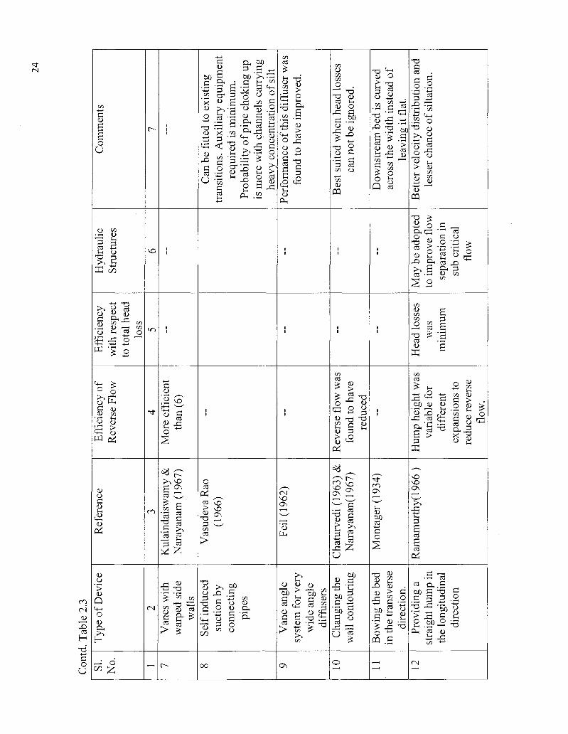
The performances of the above methods are summarized in Table 2.3

Ramamurthy et al. (1967) suggested that the use of a simple hump in an

expanding transition accelerates the flow and hence reduces flow separation and

limits the area in which the reversal of flow occurs. The present study is an

extension of concept proposed earlier. No extensive experimental study was

conducted earlier about the performance of the humps. The present study aims at

verifying the effectiveness of humps in larger expansion angles, to investigate the

19

possibility of using splitter vanes, and finally to conduct a few numerical

simulations by CFD analysis in 3-dimensional perspective.

2.8 Some previous methods of transition design

Extensive theoretical and experimental investigations on axisymmetric expansion

in pipes have been done ( Gibson et al., 1912, Chaturvedi, 1963, and Kalinske,

1946).The approaches for design of open channel expansions have comparatively

been lesser in number and more empirical in nature. Hinds (1926) was the first to

give a basis for such a design.

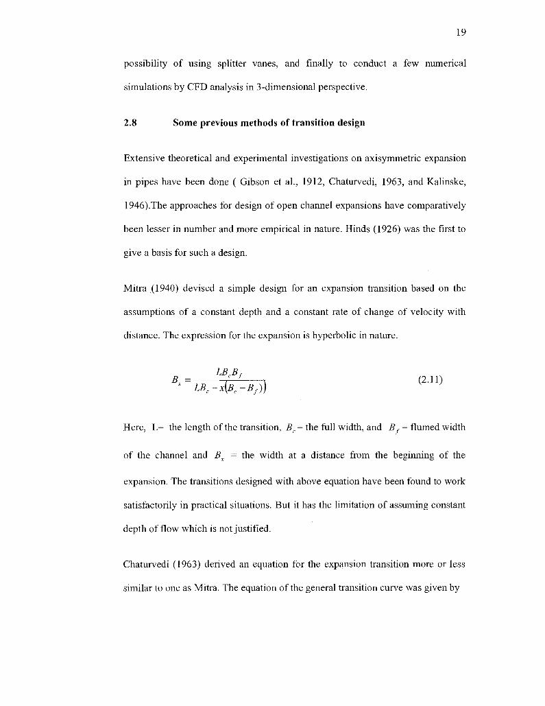
Mitra (1940) devised a simple design for an expansion transition based on the

assumptions of a constant depth and a constant rate of change of velocity with

distance. The expression for the expansion is hyperbolic in nature.

LBBf

Bx= f-L * (2.11) LBc-x(Bc-Bf))

Here, L= the length of the transition, Bc= the full width, and Bf = flumed width

of the channel and Bx = the width at a distance from the beginning of the

expansion. The transitions designed with above equation have been found to work

satisfactorily in practical situations. But it has the limitation of assuming constant

depth of flow which is not justified.

Chaturvedi (1963) derived an equation for the expansion transition more or less

similar to one as Mitra. The equation of the general transition curve was given by

20

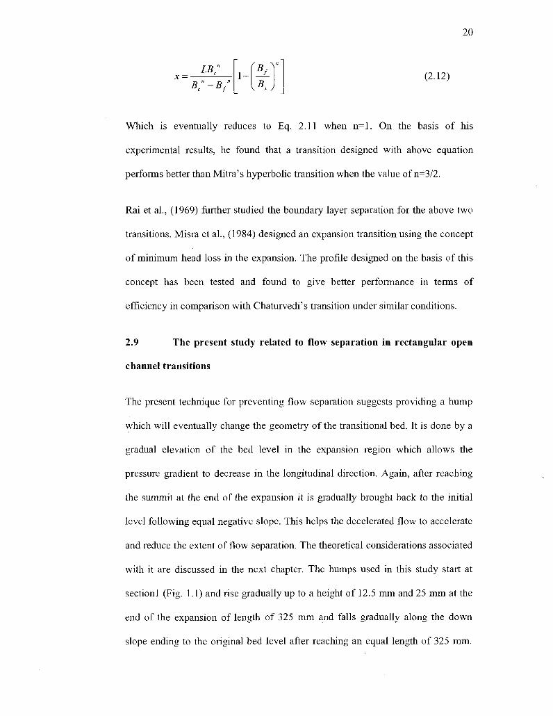
x = B:-B;

(2.12)

Which is eventually reduces to Eq. 2.11 when n=l. On the basis of his

experimental results, he found that a transition designed with above equation

performs better than Mitra's hyperbolic transition when the value of n=3/2.

Rai et al., (1969) further studied the boundary layer separation for the above two

transitions. Misra et al., (1984) designed an expansion transition using the concept

of minimum head loss in the expansion. The profile designed on the basis of this

concept has been tested and found to give better performance in terms of

efficiency in comparison with Chaturvedi's transition under similar conditions.

2.9 The present study related to flow separation in rectangular open

channel transitions

The present technique for preventing flow separation suggests providing a hump

which will eventually change the geometry of the transitional bed. It is done by a

gradual elevation of the bed level in the expansion region which allows the

pressure gradient to decrease in the longitudinal direction. Again, after reaching

the summit at the end of the expansion it is gradually brought back to the initial

level following equal negative slope. This helps the decelerated flow to accelerate

and reduce the extent of flow separation. The theoretical considerations associated

with it are discussed in the next chapter. The humps used in this study start at

sectionl (Fig. 1.1) and rise gradually up to a height of 12.5 mm and 25 mm at the

end of the expansion of length of 325 mm and falls gradually along the down

slope ending to the original bed level after reaching an equal length of 325 mm.

21

The unique advantage of using a hump is that it does not obstruct the flow along

the channel.

Another method of reducing flow separation is to provide a splitter vane system.

This method has qualitative data but there is no existing quantitative data.

Providing a vane or a system of vanes actually makes transition angle smaller.

Hence, it reduces flow separation. In the present study, data was collected with a

single vane and with a system of three vanes placed in the transition region of the

channel.

Moreover, turbulent intensity data were collected in order to develop a data bank

for validation of future simulation studies.

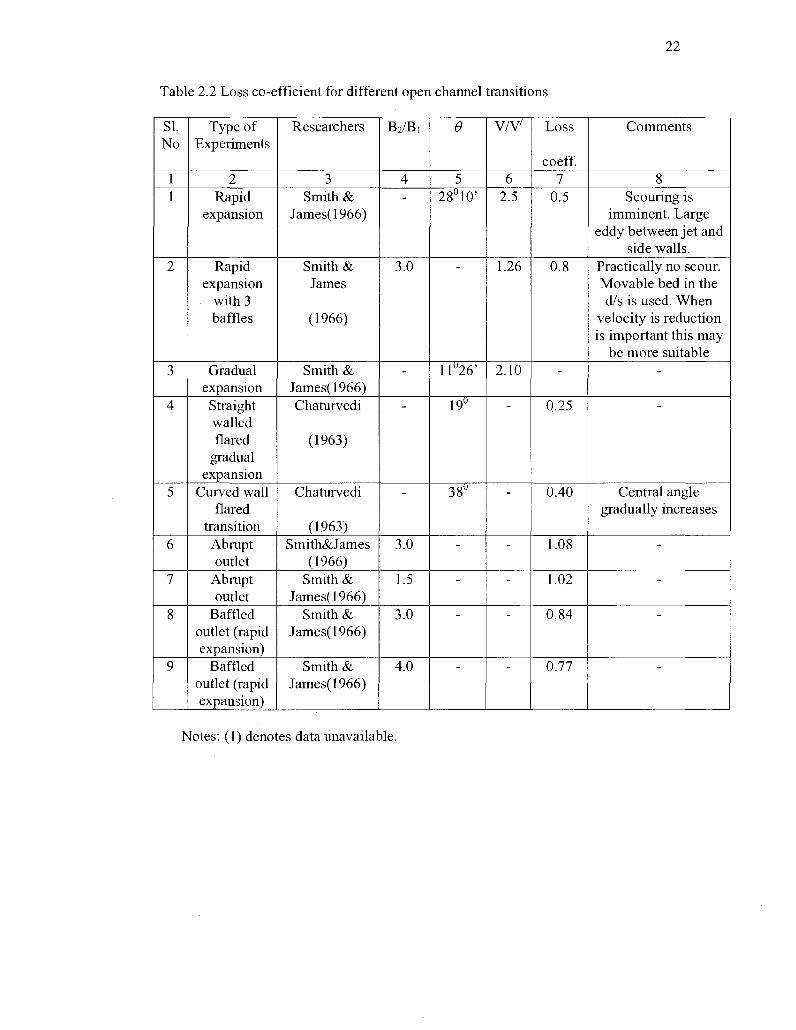
22

Table 2.2 Loss co-efficient for different open channel transitions

SI. No

1 1

2

3

4

5

6

7

8

9

Type of Experiments

2 Rapid

expansion

Rapid expansion

with 3 baffles

Gradual expansion Straight walled flared

gradual expansion

Curved wall flared

transition Abrupt outlet

Abrupt outlet

Baffled outlet (rapid expansion)

Baffled outlet (rapid expansion)

Researchers

3 Smith &

James(1966)

Smith & James

(1966)

Smith & James(1966) Chaturvedi

(1963)

Chaturvedi

(1963) Smith&James

(1966) Smith &

James(1966) Smith &

James(1966)

Smith & James(1966)

B2/Bi

4

3.0

-

3.0

1.5

3.0

4.0

9

5 28u10'

l lu26'

19°

38°

-

-

v/v'

6 2.5

1.26

2.10

-

-

Loss

coeff. 7

0.5

0.8

-

0.25

0.40

1.08

1.02

0.84

0.77

Comments

8 Scouring is

imminent. Large eddy between jet and

side walls. Practically no scour. Movable bed in the d/s is used. When

velocity is reduction is important this may

be more suitable -

Central angle gradually increases

-

-

Notes: (1) denotes data unavailable.

rsi

OO

C _ o 'oo c o3 & CD

<=! o3

o

o

c3 On 0) oo CD

o CD S-i

T3 O ,-g 15

o

g g

0 0

<N CD

03

<D

g g o O

0 0

o

I-c

X

O g <D S3 On X3

o >-< i S <- -W - 4 - * - t - »

W '> o

o c <L>

o 93

E <u oo •—

CD >

o a

0)

° o C"1 CD

-: o oo £

VO

CS

§ 2

6 <» 5 ~ a,

a .S ^•2 3

§ s O H ^ X O

CD

03

03

S 3 *

O ^ CD O

S t: 3 <D

53 > 3 o 0 3 ^ , 0 3

O ^ O O

T d 03 CD

•S J3 T d 03

g o

-° •-§ ^ ' |

^ l - c

' o

W -*—» o

c 1)

'o C*-H

<u >> J-c <D

>

O0

g 00

oo

M-l 03

CD •—

o3

O0

-a c & - 2

a 03

- 4 — »

t-c a>

CD CQ

oo ,—i 03 ^ j -<U on

^ ) o3

2 G

>. 'o 03 LC

«=5 a>

ON

o oo

oo

<N

<u

(D <L) 03

P O

O W) t+-l 03 O —'

.s Z GO a o

o

c rn 'oo

• - a

00 ^<

^ > ^ S "3

. 2 <u o 0 0 - ° ^ -oo o

<U • - 03

g * ^ 03

3 i . O

C « O o3 O „_ '+3 U

?> > o C b C *-i o d S o

<U o ; 3 3 « O oo oo

Z | o §

oo

5 O ON

• S O DO -g

oo K

S) g 03

oo ' , "O

C U Q

03 03 • c -£>

_ N C a o d O D H & ,

"2 2 x 03 _p <u

^ 1 3 03

o3

O -a

03

&H g m JO,

2 Z

J ^ « O0

II O

o3 O oo <D &0

c • >

03 J 3

a « «

g oo C

^ ^ ° T3 c a u ° _ * J C T3 oo w_ l (u "-* ^ w O0 60 g o

OO g

D a > <o > - x

CD O

ON

0>

o3

Q

o3

D H

X f

<+H O

Is o

CD

CD 03

CD c O

T d oo CD

'-£ - 4 — '

0 0

CD >

03

a"

§ 6 03 o3 oo 55 r -

1 s S C s i rf

03 ^ H

3= T3 -a

CD CD oo

c > > a, -5 12 O - r ; 'oo

CD

O cu oo > CD CD O ^ •3 oo

t d T3 CD • —

* §

O

3^ O ^ 5 *S CO t f l

CD g 0 ^ -S « 5 ^3

^O

rsi

H +^ c o U

Com

men

ts

Hyd

raul

ic

Stru

ctur

es

Eff

icie

ncy

with

res

pect

to

tota

l hea

d lo

ss

Eff

icie

ncy

of

Rev

erse

Flo

w

Ref

eren

ce

Typ

e of

Dev

ice

—; 6 C/3 £

r-

o

i n

-xT

m

(N

-

1 1 1

1 1

1

Mor

e ef

fici

ent

than

(6)

K

ulai

ndai

swam

y &

N

aray

anam

(19

67)

Van

es w

ith

war

ped

side

w

alls

r-

Can

be

fitte

d to

exi

stin

g tr

ansi

tion

s. A

uxil

iary

equ

ipm

ent

requ

ired

is m

inim

um.

Prob

abil

ity

of p

ipe

chok

ing

up

is m

ore

wit

h ch

anne

ls c

arry

ing

heav

y co

ncen

trat

ion

of s

ilt

i l

Vas

udev

a R

ao

(196

6)

Self

indu

ced

suct

ion

by

conn

ectin

g pi

pes

oo

Perf

orm

ance

of t

his

diff

user

was

fo

und

to h

ave

impr

oved

.

i

i I

i I

Feil

(196

2)

Van

e an

gle

syst

em f

or v

ery

wid

e an

gle

diff

user

s

C\

Bes

t su

ited

whe

n he

ad l

osse

s ca

n no

t be

igno

red.

I i

• i

Rev

erse

flo

w w

as

foun

d to

hav

e re

duce

d

Cha

turv

edi(

1963

)&

Nar

ayan

an(1

967)

C

hang

ing

the

wal

l co

ntou

ring

o

Dow

nstr

eam

bed

is c

urve

d ac

ross

the

wid

th i

nste

ad o

f le

avin

g it

flat

.

l l

i l

i l

Mon

tage

r(19

34)

Bow

ing

the

bed

in t

he t

rans

vers

e di

rect

ion.

—

Bet

ter

velo

city

dis

trib

utio

n an

d le

sser

cha

nce

of s

ilta

tion

. M

ay b

e ad

opte

d to

im

prov

e fl

ow

sepa

ratio

n in

su

b cr

itica

l fl

ow

Hea

d lo

sses

w

as

min

imum

Hum

p he

ight

was

va

riab

le f

or

diff

eren

t ex

pans

ions

to

redu

ce r

ever

se

flow

.

Ram

amur

thy(

1966

) Pr

ovid

ing

a st

raig

ht h

ump

in

the

long

itudi

nal

dire

ctio

n

CM

25

Table 2.4 Flow regimes in separation process (Sagi et. al., 1967)

Tuft Pattern

______^N ~~~~~~Z^>

— - ^ —4 ^ \ ~-~-4

r^—-~~~ W — "

Symbol

S

U

TI

IT

T

F

Description

Steady flow-small or no oscillations of tufts.

Unsteady flow- medium amplitude oscillations of

tufts with no back flow observed.

Incipient transitory stall- large amplitude

oscillations of tufts on the verge of the tuft

pointing upstream

Intermittent transitory stall- large amplitude

oscillations of tufts with the tuft pointing upstream

for short periods of times

Transitory stall- tuft points upstream for

approximately the same period of time as it points

down stream.

Fixed stall- Tuft points upstream for long period

of time.

26

C H A P T E R 3

EXPERIMENTAL SET UP

3.1 Physical model

3.1.1 Experimental channel

The laboratory tests were performed in a Plexiglas channel designed and built for

measuring flow velocities using LDA, having rectangular cross section. The upstream

channel was 171 mm wide and 304.8 mm deep with an overall length of

approximately 2.0 m and the down stream channel was 284.5 mm wide and 304.8 mm

deep with a length of 3.0 m. These two channels are again connected by a transition of

325 mm long and 304.8 mm deep with a width of 171 mm in the upstream and 284.5

mm in the down stream respectively.

The upstream channel was connected to a large tank with an overflow section to

diminish turbulent flow and the down stream channel was connected to exit gate

provided to control sub critical flow in the channel. The channel flow was steady due

to the overflow device. The exit flow was directed towards a V-notch to measure the

discharge Q (m3/s). The inlet to the transition was made sufficiently long (> 1500mm)

to achieve good entrance conditions and the long exit section length (> 2000 mm) was

required to get fully undisturbed flow at the end. The channel walls were made of

12.5 mm thick Plexiglas sheets and were supported by external Plexiglas flange made

of 19 mm Plexiglas at 325 mm spacing along the straight sections and 323.3 mm in

the transition.

27

Fig: 3.1. Plan of horizontal rectangular open channel transition fitted with humps

The entire channel was supported on a steel frame on a number of identical and

equally spaced steel box angle frames 1.5 m above the laboratory floor. Two wooden

platforms - one at the bottom of the channel and another one at the side of the channel

were erected to facilitate the movement of LDA traverse to measure velocity from the

bottom as well as from the side of the channel. The spacing between the supporting

sections allowed the probe to focus and measure velocities at points on the flow

fields. A steady water flow was ensured in the channel through pumping water to the

large tank with the overflow device. The experiments were conducted on two physical

setups; one with humps and the other with vanes. Two different linear humps of 12.5

mm and 25 mm high at crests were fabricated with 1.5 mm thick Plexiglas sheets

supported by wedges at the bottom. The humps were placed at the starting of

transition and reached its apex at the end of maximum transition followed by a down

28

slope of equal magnitude of the upward slope. The experimental locations were

chosen at the beginning of the transition, at the end of the transition (350 mm apart),

300 mm down stream of expanded channel.

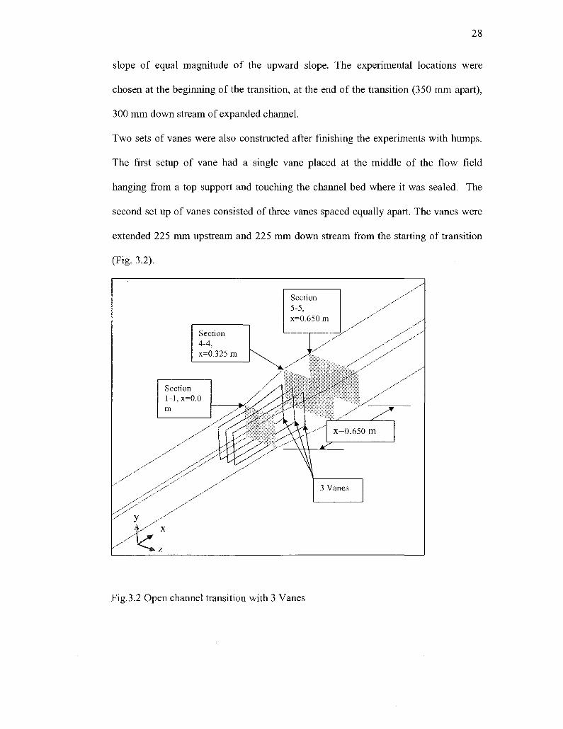
Two sets of vanes were also constructed after finishing the experiments with humps.

The first setup of vane had a single vane placed at the middle of the flow field

hanging from a top support and touching the channel bed where it was sealed. The

second set up of vanes consisted of three vanes spaced equally apart. The vanes were

extended 225 mm upstream and 225 mm down stream from the starting of transition

(Fig. 3.2).

Fig.3.2 Open channel transition with 3 Vanes

29

3.2 Instrumentation

3.2.1 Velocity measurements

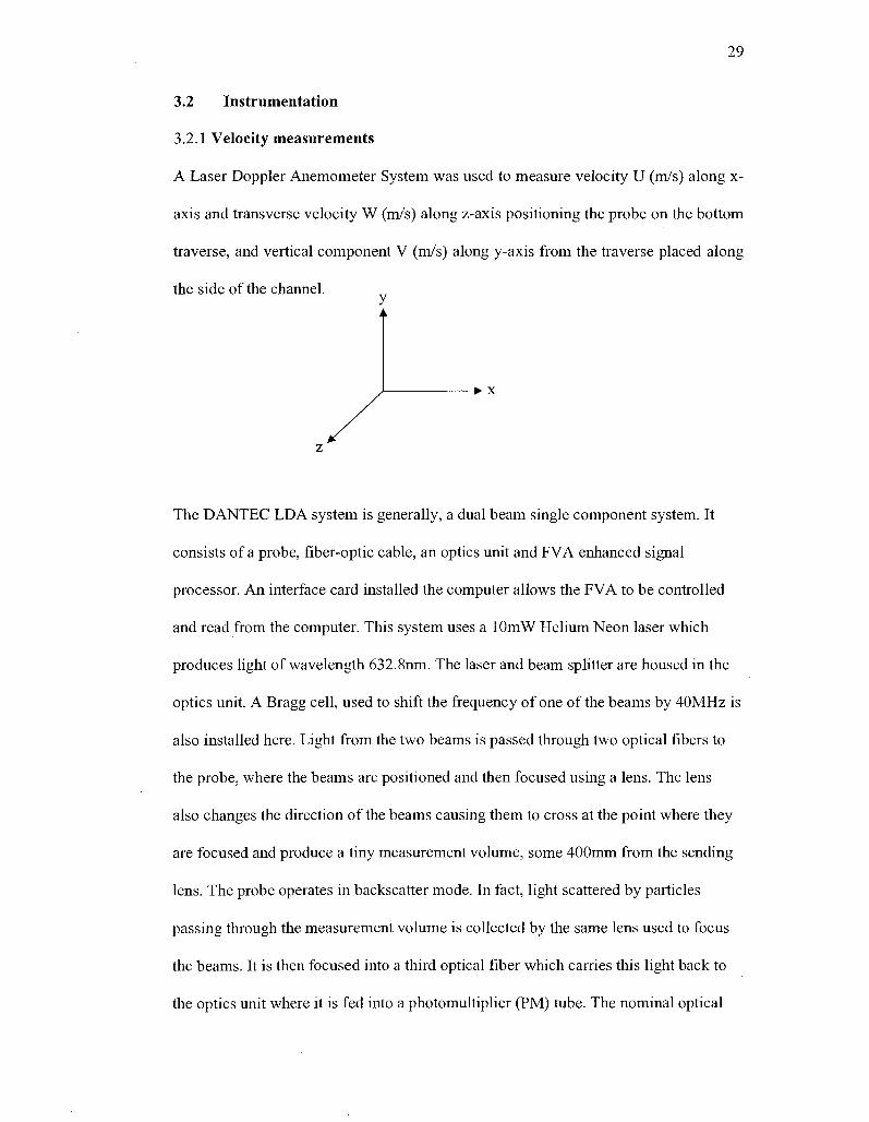
A Laser Doppler Anemometer System was used to measure velocity U (m/s) along x-

axis and transverse velocity W (m/s) along z-axis positioning the probe on the bottom

traverse, and vertical component V (m/s) along y-axis from the traverse placed along

the side of the channel.

J • X

z

The DANTEC LDA system is generally, a dual beam single component system. It

consists of a probe, fiber-optic cable, an optics unit and FVA enhanced signal

processor. An interface card installed the computer allows the FVA to be controlled

and read from the computer. This system uses a lOmW Helium Neon laser which

produces light of wavelength 632.8nm. The laser and beam splitter are housed in the

optics unit. A Bragg cell, used to shift the frequency of one of the beams by 40MHz is

also installed here. Light from the two beams is passed through two optical fibers to

the probe, where the beams are positioned and then focused using a lens. The lens

also changes the direction of the beams causing them to cross at the point where they

are focused and produce a tiny measurement volume, some 400mm from the sending

lens. The probe operates in backscatter mode. In fact, light scattered by particles

passing through the measurement volume is collected by the same lens used to focus

the beams. It is then focused into a third optical fiber which carries this light back to

the optics unit where it is fed into a photomultiplier (PM) tube. The nominal optical

30

characteristics of the system are (i) focal length = 400mm, (ii) beam separation at

sending lens= 38 mm, (iii) Gaussian beam diameter at sending lens =1.3 mm, (iv)

M measurement volume diameter = 0.248 mm, (v) fringe spacing = 6.667 m, and (vi)

number of fringes in measurement volume = 37.

Signals from the PM tube are sent to the PDA processor. The burst detection criteria

and processing parameters of the processor are set from the computer, which is also

used to read the results. The top one labeled DOPPLER MONITOR outputs the high-

pass filtered PM tube signal. The high-pass filter removes the pedestal. An

oscilloscope is connected to this signal to monitor the bursts.

The laser probe is mounted on a 3-axis traverse gear made from a milling machine

base. Being so heavy the traverse gear provides a stable means of positioning the

measurement volume at any point in the test section. The probe mount also allows the

probe to be rotated about its axis by 90 degrees, to change the component of the

velocity being measured.

In the present study more advanced DANTEC BSA Flow Software, dual PDA

version, was used to control the LDA system from the lab computer, and to collect the

velocity measurements in two directions at a time. A third party traverse system run

by another computer with the software NFTERM was used to move the probe to get

different point velocities along the test sections.

For the purpose of data collection the test sections were divided, lengthwise, in to five

sections and each section was subdivided into a grid along the channel cross sections.

The following procedures were followed prior to actual velocity measurements:

31

(i) The direction of the bisector of the two laser beams was adjusted so that it

was aligned perpendicular to the channel at the section under investigation.

(ii) The probe was then moved back and forth using the traverse controller

along the traverse gear as well as along the channel until the beams

intersected precisely at the required measuring point in the flow field.

(iii) Finally PDA software was run to take the readings moving the probe along

horizontal and vertical axes as required.

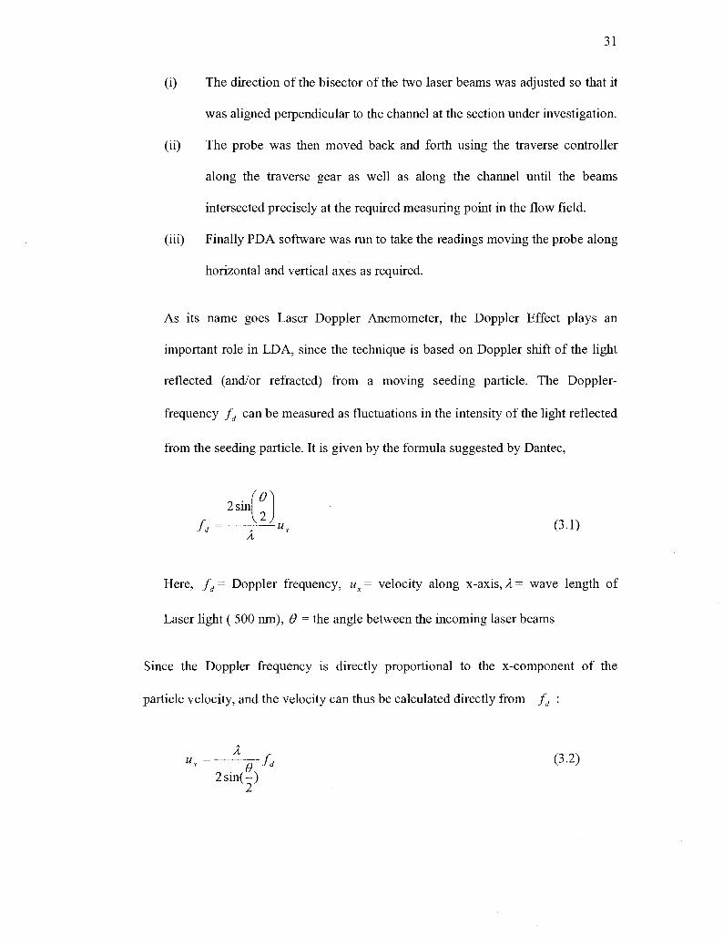
As its name goes Laser Doppler Anemometer, the Doppler Effect plays an

important role in LDA, since the technique is based on Doppler shift of the light

reflected (and/or refracted) from a moving seeding particle. The Doppler-

frequency fd can be measured as fluctuations in the intensity of the light reflected

from the seeding particle. It is given by the formula suggested by Dantec,

2 sin —

Here, fd = Doppler frequency, ux= velocity along x-axis,X= wave length of

Laser light ( 500 nm), 0 = the angle between the incoming laser beams

Since the Doppler frequency is directly proportional to the x-component of the

particle velocity, and the velocity can thus be calculated directly from fd :

ux=—^-fd (3-2) 2 sin(—)

2

32

To measure velocities, a Bragg cell is introduced in the path of one of the laser

beams. Another disadvantage is that it needs transparent flow through which the

light beams can pass, and the fact that they do not give continuous velocity

signals. Laser Doppler Anemometer offers unique advantages in comparison with

other fluid flow instrumentation. It is a non-contact optical measurement that

gives well-defined directional response, high spatial and temporal resolution, and

multi-component bi-directional measurements and requires no calibration- no

drift. The accuracy of the velocity measurements has 1% error margin.

3.2.2 Depth measurements:

In order to draw surface profiles and to compute boundary shear stresses from point

velocities, the positions of the measuring points, with respect to the channel bed and

the water surface, must be determined. Furthermore, accuracy in depth measurements

is extremely important if errors in computations of related bed shear stress are to be

minimized. Depths, surface water profiles and side water profiles were measured by a

metric depth gauge that had a resolution of 0.1 mm.

3.2.3 Pressure head measurements:

Wall pressure head measurements taken using manometers located on the walls of the

expansion section of the channels. The pressure taps were 1.6 mm in diameter. The

manometers could measure the pressure head to the nearest 0.1 mm. The manometers

displayed the static head -1 r)

. To obtain the true value, a datum was

established. The datum was the bottom elevation the channel when — =o.

33

3.2.4 Other parameters:

The water temperatures were recorded by thermometer and typical temperature

recorded was around 20° Celsius ± 2°. The flow rate Q was measured by diverting the

flow through a calibrated V-notch located in the bottom floor of the 2-storey lab. The

flow over the V-notch was measured up to the nearest 0.1 mm. The accuracy of the

discharge measurement is estimated to be 3 %. (ASME Flow meter).

34

CHAPTER 4

THEORETICAL CONSIDERATIONS

4.1 Hump and its effects:

The following assumptions are made to consider the actions of humps in suppressing

follow separation in a channel transition.

(i) The pressure distribution is hydrostatic

(ii) The original channel bed is horizontal.

(iii) Head losses are negligible since the length between two sections is small,

(iv) Energy coefficient a is unity

The effect of hump on the flow condition is explained with the use of the specific

energy diagram (Fig. 4.1). The curve 1 denoted by A'C'B' shows the energy

diagram for an open channel of uniform cross section at (l)-(l) in the upstream.

When the flow is under subcritical conditions and it passes through the expansion,

the discharge per unit width q as well as the velocity decreases (Rao, et al., 1967).

The curve for specific energy in the expansion at section (4)-(4) is shown by curve

2 denoted by ACB. Applying the energy equation, the energy at sections (l)-(l)

and (4)-(4) are constant; the positions 1 and 3 represent the same energy level and

remain in the same vertical line. Here, the velocity V2 decreases (V2<Vi) and

depth of flow Y3 increases (Y3>Yi) and thus balances the energy condition. The

flow under this decelerated state experiences adverse pressure gradient, and hence

flow separation may occur

35

* E

2g *¥ Consider two values of discharge per unit width. Therefore, two E-Y curves.

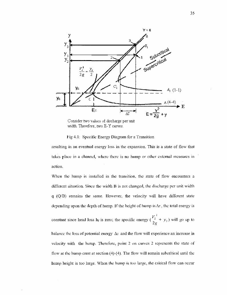
Fig 4.1: Specific Energy Diagram for a Transition

resulting in an eventual energy loss in the expansion. This is a state of flow that

takes place in a channel, where there is no hump or other external measures in

action.

When the hump is installed in the transition, the state of flow encounters a

different situation. Since the width B is not changed, the discharge per unit width

q (Q/B) remains the same. However, the velocity will have different state

depending upon the depth of hump. If the height of hump is Az, the total energy is

V2

constant since head loss hf is zero; the specific energy (— - + y2) will go up to

2g

balance the loss of potential energy Az and the flow will experience an increase in

velocity with the hump. Therefore, point 2 on curves 2 represents the state of

flow at the hump crest at section (4)-(4). The flow will remain subcritical until the

hump height is too large. When the hump is too large, the critical flow can occur

36

at the crest of the hump and supercritical flow can follow downstream. Otherwise,

the flow is subcritical and it is accelerated along the path (l)-(l) to (4)-(4) if

V2 V2 V2 V2

-^— > -^- (Fig. 4.1). If—?- < —— 5 the flow along the upward hump is under 2g 2g 2g 2g

deceleration and along the down slope of the hump additional deceleration occurs

and merges to down stream flow condition. So hump helps to gain a lower

pressure gradient is more desirable in the transition to diminish flow separation.

4.2 Velocity coefficient:

The familiar Bernoulli equation for energy is written in terms of head between

two points along the streamlines as follows:

2 2

7 , + z 1 + ^ = j ; 2 + z 2 + ^ (4.1)

In the above equation, it is assumed that the velocity is constant across the whole

section of the flow. This is never true because viscous effects make the velocity

lower near the solid boundaries than at a distance from them. If the velocity does

vary across the section, the true mean velocity head across the section

f 2 \ 2 V I V — will not necessarily be equal to -Jn— (where vm = mean velocity). Hence,

\2Sjm 2g

the use of the mean velocity in the velocity head term necessitates a kinetic energy

flux correction defined by (Sturm, T. W, 2001)

[v'dA a = ^—r~ (4.2)

The same consideration applies to the calculation of the momentum term \Qpv)m

and requires a momentum correction coefficient /? which is equal to

WdA P = 1 - l - (4-3)

v'A

37

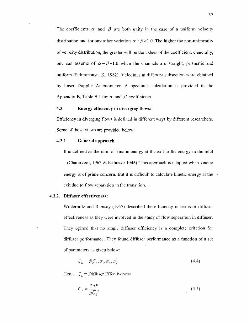
The coefficients a and /? are both unity in the case of a uniform velocity

distribution and for any other variation a > /3>\ .0. The higher the non-uniformity

of velocity distribution, the greater will be the values of the coefficient. Generally,

one can assume of a = /3=l.O when the channels are straight, prismatic and

uniform (Subramanya, K. 1982). Velocities at different subsection were obtained

by Laser Doppler Anemometer. A specimen calculation is provided in the

Appendix-B, Table B.l for a and /? coefficients.

4.3 Energy efficiency in diverging flows:

Efficiency in diverging flows is defined in different ways by different researchers.

Some of those views are provided below:

4.3.1 General approach

It is defined as the ratio of kinetic energy at the exit to the energy in the inlet

(Chaturvedi, 1963 & Kalinske 1946). This approach is adopted when kinetic

energy is of prime concern. But it is difficult to calculate kinetic energy at the

exit due to flow separation in the transition.

4.3.2. Diffuser effectiveness:

Wintermitz and Ramsay (1957) described the efficiency in terms of diffuser

effectiveness as they were involved in the study of flow separation in diffuser.

They opined that no single diffuser efficiency is a complete criterion for

diffuser performance. They found diffuser performance as a function of a set

of parameters as given below:

£D=<f>(Cp,a],a4,A) (4.4)

Here, C,D = Diffuser Effectiveness

C . = ^ (4.5) P

38

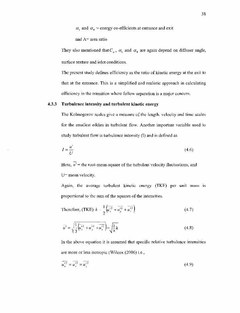
ax and a4 = energy co-efficients at entrance and exit

and A= area ratio

They also mentioned that Cp, ax and a4 are again depend on diffuser angle,

surface texture and inlet conditions.

The present study defines efficiency as the ratio of kinetic energy at the exit to

that at the entrance. This is a simplified and realistic approach in calculating

efficiency in the transition where follow separation is a major concern.

Turbulence intensity and turbulent kinetic energy

The Kolmogorov scales give a measure of the length, velocity and time scales

for the smallest eddies in turbulent flow. Another important variable used to

study turbulent flow is turbulence intensity (I) and is defined as

/ = - (4.6) U

Here, u = the root-mean-square of the turbulent velocity fluctuations, and

U= mean velocity.

Again, the average turbulent kinetic energy (TKE) per unit mass is

proportional to the sum of the squares of the intensities.

Therefore, (TKE) k = -\u'x2 + u'

2 + «f ) (4.7)

^L:2+M;2+M:2)=pfe (4.8)

In the above equation it is assumed that specific relative turbulence intensities

are more or less isotropic (Wilcox (2006) i.e.,

u =u =w, (4.9)

39

4.3.4 Boundary shear stress distribution

Measuring boundary shear stress distribution is very important in hydraulic

engineering problems like scour, bed and bank protection, sediment transport and the

design of hydraulic structures in channel transition. Applying an average value of bed

shear stress criteria is not practical in sediment transport. It may lead to either

underestimate or over estimate local values of shear. Hence, there may be either no

transport or high transport of sediment because of local shear. Earlier investigators

emphasized to determine local shear stress to overcome this problem. There are

various methods to determine boundary shear stress. Here, three methods will be

employed to compare the results with each other.

Chow (1959) used the average shear formula at the channel bottom.

T = yRS (4.10)

Here, X= boundary shear stress, y- Unit weight of water, R= hydraulic radius, S

=slope of the energy gradient line.

However, the boundary shear stress is not uniformly distributed along the wetted

perimeter except for uniform wide open channel and closed pipe flow. Hence, it is

necessary to determine local boundary shear stress in open channel. Boundary shear

stresses are generally small in magnitude and accurate measurements are difficult.

The shear within the boundary layer thickness can be calculated using the formula,

(Schlichting, 2000),

du . .. .. x

T = H— (4.11) ay

here, x=shear stress, u=molecular viscosity, du=velocity and dy= distance of the point from the bed.

Later on some researcher used the logarithmic law outside viscous sub-layer to

calculate shear velocity, and from shear velocity relation, shear stress was calculated.

40

The logarithmic equation can be written, regardless of smooth, transitional or rough bed, in the form, (Hollingshead, 1972)

/ I = «r = i ^ ^ L (4.12)

Here, ui, U2 are time averaged velocity measured at yi and y2 distances from the bed,

A =5.75 constant. Shear velocity uT is obtained by solving the right hand side of the

above equation. Hence, shear stress T is obtained equating the LHS with RHS of

equation (4.12).

4.3.5 The Reynolds number

The Reynolds number is described as the ratio of the inertial force to the viscous force

in the pipe or channel. The Reynolds numbers are determined by (Chow, 1959),

R e = ^ (6.13)

V

Here, U is the average velocity at section x = 0.0 m (Entry) in the transition channel,

R is the hydraulic radius defined by the cross-sectional area A divided by wetted A u

perimeter P i.e., R = — , and v is the kinematic viscosity (v = — ). P p

4.3.6 Froude number

The Froude number is defined as the ratio of the inertial force to the gravity force in

the flow. It is determined as the ratio between mean flow velocity, V, and the speed of

a small gravity (surface) wave travelling over the water surface (Hwang, 1996).

Therefore, Froude number is

Fr=4= (6-14)

Here, g is the acceleration due to gravity and D is the hydraulic depth.

41

When Fr =1, the flow is in the critical state, when Fr < 1, the flow is subcritical and

when Fr >1, the flow is supercritical.

42

CHAPTER 5

5.0 3D NUMERICAL CFD SIMULATIONS

5.1 CFD modeling

The three most powerful tools of fluid dynamics are experiments, partial differential

equations (PDEs), and dimensional analysis. Earlier fluid flow investigations were

largely experimental and only very simple fluid flow could be numerically solved.

With recent advances in computing techniques and numerical solution methodologies,

CFD (Computational Fluid Dynamics) has now been widely used in various industry

applications. Despite its wide application, CFD has recently been used in river flow

research and modeling hydrology and morphology by Nezu and Nakagawa, 1993;

Lane, 1998; Maetal., 2002; Cao et al., 2003, etc. (Ingham, D. B. et al., 2005). CFD

can be an alternative to physical modeling in many areas including open channel flow,

river morphology, flow structures and sediment transport and can be used in river

management and flood prediction with its advantage of lower cost, time and

flexibility.

5.2 Computational fluid dynamics (CFD)

Computational fluid dynamics (CFD) is the science (and art) of predicting fluid flow,

heat transfer, mass transfer, chemical reactions and other related phenomena by

solving mathematical equations that represent physical laws, using a numerical

process. CFD is an equal partner with pure theory and pure experiment in the analysis

and solution of fluid dynamics problems. The physical aspects of any fluid flow are

governed by the following three fundamental principles:

• Mass is of a fluid conserved

43

• The rate of change of momentum equals the sum of the forces on a fluid

particle (Newton's second law)

• The rate of change of energy is equal to the sum of the rate of heat addition

to and the rate of work done on a fluid particle (first law of

thermodynamics).

These physical principles can be expressed in terms of mathematical equations, which

are either integral or partial differential equations. Computational fluid dynamics is

the art of replacing the governing integral equations or partial differential equations of

fluid flow with numbers, and advancing these numbers in space and/or time to obtain

a final numerical description of the complete flow filed of interest. The end product of

CFD is indeed a collection of numbers in contrast to a closed form of analytical

solution. The objective of most engineering analysis is a quantitative description of

the problem, i.e., numbers. Computers have been used to solve fluid problems for

many years. Initially CFD was a tool used exclusively in research and now-a-days

increasingly it is becoming a vital component in the design of industrial products and

process due to recent advances in computing power, together with 3D graphics,

numerical algorithm, and availability of cheap and robust commercial solvers.

Therefore, CFD is now an established industrial design tools. Despite advances in

other branch of engineering, hydraulic engineering lags behind in using CFD. But

CFD can be very demanding field in modeling river flow phenomena because of the

complexity of the irregular bank and bed topographies as well as enormous volume

involved in natural river system.(Ingham, et al., 2005). However, the current concerns

of issues to be addressed in CFD simulations are grid resolution, grid dependence,

wall roughness and appropriate turbulence models (Hardy et al., 1999). Nevertheless,

CFD simulations have the capability to provide the better understanding the flow

44

characteristics of open channel flow and design inputs to control flow separation in

transitional flow.

5.3 Organization of CFD Codes

Most of the commercial CFD codes include user interfaces to input problem

parameters and examine the output. Hence all codes essentially contain three main

elements viz., a pre-processor, a solver and a post-processor. The pre-processor

defines the geometry of the region of interest, generates grid/mesh, defines fluid

properties and specifies the boundary conditions. The solver sets up the numerical

model, approximates the unknown flow variables, discretizes the governing equations,

solves the algebraic equations, computes and monitors the solution. There are three

main streams of numerical solution techniques: finite difference, finite volume and

finite element. The main difference among the three separate streams is associated

with the way in which the flow variables are approximated and with the discretization

processes. Among the three finite volume methods, finite volume method is the most

well-established and thoroughly validated general purpose CFD technique. All five

main commercially available CFD Codes viz., ANSYS CFX, FLUENT, FLOW3D,

PHOENICS and STAR-CD are using the finite volume method. The post-processor

examines and displays the result with data visualization tools and considers revisions

of the model, if necessary. At the end of a simulation the user must make judgment

whether the results are "good enough". It is not easy to assess the validity of the

models of physics embedded in a program as complex as a CFD codes or the accuracy

of its final results unless making comparison with experimental investigations. One

should bear in mind that CFD is no substitute for experimentation, but a very

powerful supplementary problem solving tool. In this study in addition to main

laboratory investigation, a few CFD analyses were done using the commercial

45

software ANSYS CFX to compare the laboratory investigation and in other words, to

validate the CFD simulation by laboratory experiment.

5.4.0 Basic governing equations

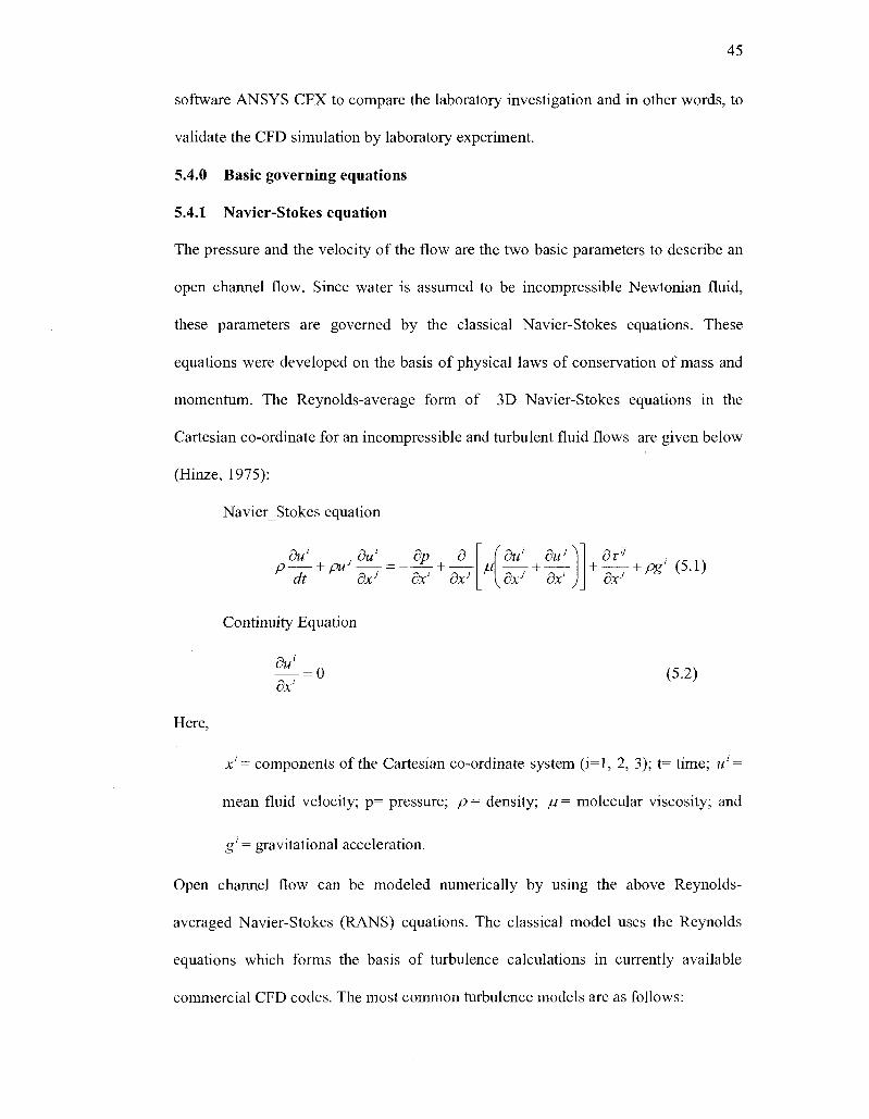
5.4.1 Navier-Stokes equation

The pressure and the velocity of the flow are the two basic parameters to describe an

open channel flow. Since water is assumed to be incompressible Newtonian fluid,

these parameters are governed by the classical Navier-Stokes equations. These

equations were developed on the basis of physical laws of conservation of mass and

momentum. The Reynolds-average form of 3D Navier-Stokes equations in the

Cartesian co-ordinate for an incompressible and turbulent fluid flows are given below

(Hinze, 1975):

Navier_Stokes equation

du' du1 du' i du' dp d P + pUJ

r = — + r dt dx' dx' dx]

M dx1 dx'

dr" + j + Pg' (5.1)

ox'

Continuity Equation

— = 0 (5.2) dx'

Here,

x = components of the Cartesian co-ordinate system (i=l, 2, 3); t= time; u' =

mean fluid velocity; p= pressure; p = density; ju = molecular viscosity; and

g' = gravitational acceleration.

Open channel flow can be modeled numerically by using the above Reynolds-

averaged Navier-Stokes (RANS) equations. The classical model uses the Reynolds

equations which forms the basis of turbulence calculations in currently available

commercial CFD codes. The most common turbulence models are as follows:

46

Classical Models based on (time-averaged) Reynolds equations

1. Zero equation model-mixing length model

2. Two-equation model k - s and k-co mode

3. Reynolds stress equation model

4. Algebraic stress model

Large Eddy simulation based on space-filtered equations

Of the classical models the mixing length and two-equation k-s and k-co

models are the most popularly used and validated models.

5.4.2 Two-equation model k-s and k-co

Despite recent sophisticated models like the RSM (Launder et al., 1975), the two

equation models are still popular turbulence models because of their easy

implementation, economy in computation and accuracy in solution with the available

computer power. The Standard k-s model (Launder and Spalding (1972) has

enjoyed popularity among the turbulence modelers. It represents the eddy viscosity by

turbulent kinetic energy k and dissipation rate co as follows:

k2

M,=cMp— (5-3) s

Here, cp= 0.09, an empirical constant

The turbulent kinetic energy k and the dissipation rate co have to obtained by solving

the following equations,

Kinetic energy equation

dk , dk d O h OUJ 7 - "

dt dxJ dx'

' ju + juA dk

V Gk ) d x '

+ P-ps (5.4)

Here,

P = ju + M,) du' du1

+ • du1

a*7 ^dxJ dx' ,

and it represents the production of turbulence.

Dissipation rate equation

ds , ds d p— + puJ — r = — :

dt dxJ dx'

M + M,

V °e J

ds dx' £i k s2 k

47

(5.5)

(5.6)

Here, csl=1.44, ce2=1.92, a , =1.0, <7e=1.3

Similar to k-s model, the k-co models are derived for the turbulence kinetic energy

k and the specific dissipation rate co = — and the turbulent viscosity is calculated by, k

M, =aP~ co

(5.7)

The first k-co model was proposed by Kolmogorov (1942). However, the models of

Wilcox (1988, 1998) and Mentor (1994) were used and tested extensively.

5.4.3 Boundary conditions

The two equations k - e model is elliptical in nature and it requires boundary

conditions on all the boundaries of the solution domains to solve the equations. The

boundary conditions to be used should reflect the real conditions to achieve the

accuracy of the model. For channel flow the following boundary conditions are

required:

(i) Inlet boundaries

(ii) Outlet boundaries

(iii) Free surface boundaries

(iv) Wall functions

48

5.4.4 Inlet boundaries

Fluid velocity and turbulence quantities are specified at the inlet boundary. A

uniform boundary profile is chosen when the inlet boundary is located sufficiently

upstream of the sections under investigation to get a fully developed flow. Great care

should be taken to select a development length since this may be large in some cases.

5.4.5 Outlet boundaries

The down stream boundary is also taken on a location where the velocity is fully

developed and the gradient is zero. When flow can not be treated as fully developed,

the pressure condition may be used and the outlet pressure is set to zero. To find the

surface profile, the outlet boundary condition needs the water surface level to be

specified.

5.4.6 Free surface boundaries

In open channel simulation, the free surface boundary is very important. For steady

state flow condition with horizontal free surface, a fixed lid method is used to

represent water surface. Various methods are employed to find the free surface. These

are classified into two major groups (Ferziger, 2002) viz., (a) Interface-Tracking

Scheme and (b) Interface-Capturing Scheme

5.4.7 Interface-tracking scheme

Sharp interface is defined in this method and the model tracks the motion of the free

surface in the computation. Frequent grid adjustments are required for unsteady free

surface. Very small time steps and boundary-fitted grids are used in this method to

find sharp interface

The boundary for the vertical velocity is determined by following equation:

dH dH dH u. = \-ux \-uv- P-oj

dt A dx "' dy

49

Here, ux, uy, and uz are the flow velocity in x-direction, y-direction, and z-direction

respectively. H is the water depth and t is the time.

The pressure variable p is determined by the following equation:

p = Po + yH (5.9)

Here, po is the free surface pressure, and y is the specific gravity (Meselhe and

Sotiropoulos, Huang et al., 2002).

5.4.8 Interface-capturing scheme

The Volume of Fluid (VOF) method is one of the Interface-capturing methods, which

does not specify any sharp boundary (Hirt and Nicholas, 1981). Though it was

designed for solving unsteady fluid problem, it is also used to predict a steady flow

while water level is not known. The VOF method can be used to determine the

surface profile using control volume method. In this method, a water volume fraction,

F, can be defined by,

F = ^ (5.10)

Here, 5Qcen is the volume of the computational cell and 5Qwater is the fraction of the

volume of the cell filled with water. Thus, the VOF equation is

F= 1, when cell is full of water

F = 0, when cell is full of air

0<F<1, when cell contains free surface.

5.4.9 Wall functions

Fluid flow near to the channel wall (bed and bank) is generally very complex in

respect of both its mean and turbulent structure. A very fine grid near to these

boundaries is required to simulate their effect on the fluid flow. Launder and Spalding

50

(1974) proposed the standard wall function to find the characteristics of mean fluid

flow region and to avoid the use of expensive and complex fine grid in the vicinity of

the wall boundaries. The standard wall function, which relates the local shear stress

(through uT ) to the mean velocity, turbulence kinetic energy and rate of dissipation,

can be expressed as follows:

^ = I l n ^ + C (5.11) UT K V

Here, u is the velocity parallel to the wall at the first cell, uT is the friction velocity, k

= 0.41, y = distance normal to the wall, v is the kinematic viscosity and C = 5.0 for

smooth walls. The effect of roughness has to be considered for rough surface and the

value of constant C has to be adjusted accordingly.

5.4.10 Grid generation

Grid generation is one of the difficult tasks to solve partial differential equations on a

complex domain such as the geometry of anur open channel transition. Boundary-

fitted orthogonal grids and curvilinear coordinates are generally employed to simulate

flows in complex geometries. These are classified as structured, block-structured, or

unstructured. In this study multi-block structured grid method is used. This method

divide the geometry in to several blocks and each block is again meshed by power law

function. It creates fine mesh near the channel transition or near the walls or in the

unsteady flow region.

CHAPTER 6

51

6.0 DISCUSSION OF RESULTS

6.1.0 Experimental results

Velocity measurements were carried out in the open channel transition with the 66%

expansion. The upstream flow conditions were subcritical and the Froude number

range was from 0.17 to 0.41. The variation of flow rate was from 0.0070 m /s to

0.0168 m3/s. The Reynolds number Re varied from 27,000 to 109,000 representing the

turbulent flow regime. The channel transition can trigger flow separation causing

energy losses. To reduce the effect of separation, the use of a hump (rising of bed

level) or vanes were explored by measuring the velocity profiles and turbulence

intensities in the section downstream of the transition. Moreover, the primary

parameters like Reynolds numbers were varied and the study determined the velocity

coefficient a and the momentum coefficient j3, turbulent energy and the regions of

reverse flow were investigated. The data obtained from LDA measurements of the

velocity were analyzed and velocity profiles were drawn.

Fig.6.1 shows the velocity contours for axial velocities at the entry section at x = 0.0

m, near the exit section at x = 0.325 m and a section in the channel slightly down

stream of the channel transition at x = 0.650 m for a specific flow condition (Q =

0.0070 m/s). Figs. 6.2 to 6.15 provide the velocity contours and the velocity

distribution near the bed and free surface for several other flow conditions (0.0070 <

Q < 0.0168). Figs. 6.16 to 6.24 represent the turbulent kinetic energy; Figs. 6.25 to

6.33 depict the turbulent intensities.

52

Table 6.1 Flow characteristics of laboratory experiments

Measurement locations X^ - 0.0 m (Entry) and X2 = 0.325 m (Exit)

Discharge

Q(m 3 /s)

Xx = 0.0133

X2 = 0.0133

Xj = 0.0168

X2 = 0.0168

Xj = 0.0160

X2 = 0.0160

Xi =0.0158

X2 = 0.0158

Xi = 0.0070

X2 = 0.0070

Xx = 0.0110

X2 = 0.0110

Xt = 0.0142

X2 = 0.0142

Xx = 0.0072

X2= 0.0072

Velocity

v (m/s)

0.492

0.273

0.551

0.325

0.592

0.327

0.541

0.285

0.282

0.161

0.227

0.389

0.488

0.271

0.284

0.273

Channel Depth

D(m)

0.158

0.171

0.178

0.182

0.158

0.172

0.171

0.195

0.145

0.153

0.170

0.165

0.170

0.185

0.148

0.154

Froude No

Fr

0.395

0.211

0.417

0.243

0.475

0.251

0.416

0.206

0.236

0.130

0.175

0.306

0.378

0.201

0.236

0.222

Reynolds No

Re

86,575

52,042

109,275

65,795

104,150

62,563

102,714

61,819

45,484

27,230

42,925

71,543

92,375

55,562

46,836

46,834

6.1.1 Reynolds number effect

Froude number is a primary parameter of subcritical open channel flow. However, its

influence was restricted due to its narrow range of variation (Table 6.1) in the tests.

Moreover, since the experimental channel flow is highly turbulent in nature, the

Reynolds number here plays a role to characterize the dynamics of flow separation

including the distribution of velocity, turbulent kinetic energy and turbulent intensity.

Experimental evidence shows that the point of separation around a sphere or rounded

bluff body can be moved downstream when the boundary layer flow becomes

turbulent. When turbulence is increased by mechanical devices like tripping rings, the

channel flows turn more turbulent giving the desired movement of separation point

53

(Schlichting, 2000). However, for flow past a channel expansion of the present case

separation point is fixed and hence effect of Reynolds number is not extensive. Still

the extent of separation depends on the factors such as the divergence angle, and the

shape of the transition. It may be a straight transition or a curved transition. Flow

visualization by dye techniques can give the downstream point of reattachment in

some cases. As the dye diffused in the flow very quickly, the procedure of dye

technique to locate point of separation was not successful. One can use a tuft to locate

the reattachment point.

6.1.2 The energy coefficient a and momentum coefficient f3

Table 6.2 shows the variations of a and/?. In each case, the flow separation zone is

seen at section 4-4. The values of a and j3 are larger at section 4-4, but those are

much smaller at sections 1-1 and 5-5 as expected. In the later case, the flow has

recovered slightly.

Table 6.2 Variation of a and P with Reynolds Number

SI. No

1

2

3

4

5

6

7

8

9

10

11

12

13

Discharge

Q (m3/s)

0.0110

0.0133

0.0070

0.0142

0.0158

0.0070

0.0168

0.0070

0.0158

0.0142

0.0070

0.0142

0.0070

Inlet

Re No

71543

86575

45484

92375

102714

46836

109275

46836

102714

92375

46836

92375

46836

Inlet

F rNo

0.31

0.40

0.24

0.38

0.42

0.24

0.42

0.24

0.42

0.38

0.24

0.38

0.24

Values of a

Section

1-1

a

1.00

1.07

1.01

1.08

1.01

1.08

1.08

1.08

Section

4-4

a

1.10

N/A

1.31

1.23

1.44

1.23

1.27

1.16

1.32

1.42

1.30

1.21

1.31

Section

5-5

a

1.05

N/A

1.18

1.18

1.28

1.23

1.15

1.27

1.09

1.11

1.15

1.01

1.09

Values of (3

Section

1-1

P

1.00

1.02

1.00

1.03

1.00

1.03

1.03

1.03

Section

4-4

P

1.03

1.11

1.07

1.15

1.10

1.10

1.06

1.13

1.16

1.11

1.08

1.11

Section

5-5

P

1.01

1.06

1.06

1.11

1.08

1.04

1.11

1.03

1.04

1.05

1.00

1.03

Comments

No Hump

No Hump

No Hump

No Hump

No Hump

12.5 mm Hump

12.5 mm Hump

25 mm Hump

25 mm Hump

1 Vane

1 Vane

3 Vanes

3 Vanes

55

6.1.3 Velocity distribution and percentage area of reversal flow

The present study investigated the effectiveness of the hump and vane to reduce flow

separation at the channel expansion under subcritical flow regime. Efforts were made

to quantify the reverse flow region due to flow separation to some extent for different

flow conditions considering the rate of flow, with and without auxiliary devices

(humps and vanes). The results given in the Table 6.3 show the level and extent of the

reverse flow observed at the exit of the transition (x = 0.325 m) for different flow

rates considering other variables.

Table 6.3 Variation of % of area of reverse flow field with inlet Reynolds number

SI. No.

1

2

3

4

5

6

7

8

9

10

11

Discharge Q inm3/s

0.0070

0.0142

0.0158

0.0070

0.0168

0.0070

0.0158

0.0072

0.0142

0.0072

0.0142

Inlet Reynolds No. R^ X10"

4.54

9.23

10.27

4.68

10.41

4.68

10.27

4.68

9.23

4.68

4.68

Area of Flow At Section 4-4 m2

0.04345

0.05310

0.05339

0.04061

0.00000

0.03777

0.04970

0.04430

0.05254

0.04430

0.05026

Area of Reverse Flow Field at Sec.( 4-4)

m2

0.0060

0.0040

0.0015

0.00006

0

0

0

0.0003

0.0008

0

0

% of Reverse Flow

14

8

3

0.1

0

0

0

1

1

0

0

Remarks

Fig.6.1(b), No Hump Fig.6.3(b), No Hump Fig.6.4(a), No Hump Fig.6.5(b), 12.5 mm Hump Fig.6.6(b), 12.5 mm Hump Fig.6.7(b), 25 mm Hump Fig.6.8(b), 25 mm Hump Fig.6.9(b), 1 Vane Fig.6.10(b), 1 Vane Fig.6.11(b), 3 Vanes Fig.6.12(b), 3 vanes

56

Figs. 6.2a to 6.4c denote the flow behavior in the transition for three different flow

rates (Q = 0.0133 m3/s, Q = 0.0142 m3/s, and Q = 0.0158 m3/s).

In all these cases, neither the hump nor the vane was present. Reverse flows were

concentrated at the corners at section 4-4. It may be recalled that above figures show

no reverse flow at the entry section and at the section down stream of the transition.

The variations of velocity near the free surface (top) and near the floor (bottom) are

also included in Fig.6.5 for two different flow rates. Figures 6.5a and 6.5b show the

velocity distribution near the bottom and near the surface of water and the negative

values indicate the reversal of flow.

6.1.4 Transition flow characteristics with a hump

Fig. 6.6 shows the characteristics of velocity for transition flow with a hump in place.

It shows that even a small hump (12.5 mm hump) reduces the flow separation

significantly (Fig6.6b). Fig. 6.7 shows the flow behavior for the same hump height of

12.5 mm at Q = 0.0160 m3/s. and Figs. 6.8(b) and 6.9(b) show that a larger hump

height (z = 25 mm) removes the separation totally. As before the velocity distribution

near the bottom surface and near the surface of water are shown in Figs. 6.10a to

6.11b. The disappearance of negative values indicates that the flow separation is not

present.

6.1.5 Effect of Vane on Transition Flow Characteristics

Figs. 6.12 and 6.13 show the effect of a single vane, and Figs.6.14 and 6.15 show the

effect of 3 vanes in the transition. A single vane reduced the flow reversal to 1 % from

57

that of flow without vane a (14%). Further, it was found that the three vanes were

more effective than the single vane. One vane reduced separation significantly but 3

vanes completely removed separation. The study revealed that the percentage of

reversal flow is much less than that in a smaller expansion as found in the past

preliminary studies. (Rao, 1967 and Ramamurthy et al. 1967). In the past studies of

Rao (1967), the end of channel boundary conditions were different and the velocity

data was collected by Pitot tubes which are not very effective for reverse flow

measurement. In the present case, LDA was used to measure velocity. The most

striking feature of the velocity distribution is that though the channel section is

symmetrical, the flow distribution in the transition is unsymmetrical.

6.1.6 Turbulent Kinetic Energy and Turbulence Intensities

Figs. 6.16 to 6.18 show the distribution of turbulent kinetic energy for 3 different flow

rates when no hump was present. Figs. 6.19 to 6.22 show the kinetic energy data at

different sections for transition flows with humps. Lastly, Figs. 6.23 to 6.24 provide

kinetic energy data for transition flows with vanes.

Figs.6.16 to 6.24 and Figs. 6.25 to 6.33, represent turbulent kinetic energy (TKE)

associated with the open channel transition flow and the turbulence intensity (TI)

distributions respectively at the three sections with neither the hump nor the vane and

a hump (Az=12.5 or 25 mm) and the two systems of vane (1 and 3 vanes). These data

refer to both the maximum and minimum flows of 0.0158 and 0.007 (m3/s). Since at

the exit section (x = 0.325 m), flow separation was present due to channel expansion,

turbulence data was collected there. The intensity of turbulence sketches and the

turbulent kinetic energy sketches are nearly similar. As such, only the former are

discussed in details in the following section.

58

6.1.7 Turbulence Intensity Diagrams

Fig. 6.25 shows the intensities for minimum flow condition of 0.007 (m /s) and

without use of hump. Here, the observed intensities were 0 - 0.8 at section 4-4 and 0-

0.3 at section 5-5 and maximum intensities were near the walls.

In Fig. 6.26, it was also observed that the turbulent intensities with a range of 0-1.0

are high at section 4-4 (Fig.6.26b) in comparison to other two sections 1-1 and 5-5

with the range of 0-0.35 and 0-0.8 respectively. The turbulent kinetic energy and

intensities were highest at surfaces in section 4-4 and 5-5 and at sides in section 1-1.

The middle area experienced the lowest intensities. Mehta (1981) and later El-Shewey

and Joshi (1996) conducted the study of the effect of channel expansion on turbulence

characteristics. In Figs. 6.26b and 6.26c, the maximum turbulence intensities occurred

either close to free surface or close to bottom which agreed with the findings of

Brundette and Baines (1985) and El-Shewey and Joshi(1996). They state that

turbulent intensities increase toward the free surface indicating the transfer of a

higher-momentum flux from the channel bed to the free flow surface.

Fig. 6.27 represents turbulent intensities data for another case of without hump or

vane situation. Here the flow rate was 0.0158 (m3/s) with higher Reynolds numbers.

The turbulent intensity ranges were 0 to 0.6 and 0 to 0.4 at section 4-4 and 5-5

respectively. The highest intensities were clustered near the walls.

The use of 12.5 mm hump reduced the intensity levels to 0-0.30 and 0-0.25 at section

4-4 and 5-5 respectively (Fig.6.28). The percentage reductions were 62% and 16%.

The maximum turbulent intensities were close to the walls i.e., the intensity increased

with depth.

59

Fig.6.29 denotes the turbulent intensities at section 4-4 and 5-5 with 12.5 mm hump

(Q = 0.0168 m3/s). The intensity ranges were 0-0.25 and 0-0.20 and the high cores

were near the walls.

Fig. 6.30 represents a case with 25 mm hump and a flow rate of 0.0070 m3/s. Here the

intensities were in the range of 0-0.20 at exit section and 0-0.15 at the down stream

section. The maximum intensities were observed near the walls.

Fig. 6.31 shows two sections at 4-4 and 5-5 with the use of 25 mm hump. Here, the

ranges of turbulent intensities were 0-0.2 and 0-.0.20. So, the reductions were 67%

and 50% respectively. The maximum intensities were observed near the bottoms and

corners.

Fig. 6.32 indicates the turbulent intensity distribution for the present study (Q=0.142

m3/s) while using a one splitter vane at the centre. The use of a splitter vane was

effective in decrease of turbulent intensities in the range of 0 to 0.3 at section 1-1, 0 to

0.7 at section 4-4 and 5-5. Further at sectionl-1, 4-4 and 5-5, the reduction of

turbulent intensities was about 14%, 30% and 25% respectively. This trend tells us

that the decrease of turbulence intensity indirectly indicates a reduction of flow

separation. Here the maximum intensities were shifted to either the side or floor of the

channel and the minimum was at the middle.

Fig.6.33 represents the use of 3 vanes placed at equal distance apart and here the

intensity decrease trend is similar to that of one vane. The maximum intensities

occurred at the sides of the sections.

Intensity distribution patterns also suggest that the flow was anisotropic throughout

the depth. Turbulent anisotropy is the primary process triggering secondary flows of

Prandlt's second kind (Nezu and Nakagawa 1993).

60

It was also found that a channel expansion created an unbalanced turbulent kinetic

energy distribution, thus affecting the distribution of intensities. This result agrees

with the findings of Mehta(1981) and El-Shewey and Josho (1997) who studied flows

with sudden expansions. The maximum turbulent intensities were found to occur near

the free surface, at the sides and above the bottom. In their studies the intensity

increased with depth suggesting that turbulence momentum is not transferred from the

core of flow to the bed, but from the bed to the free surface. This indicates the

presence of secondary flows of the second kind due to channel expansion (Ead et al.

2000).

Proper use of vane and hump can reduce flow separation and hence reduce intensity

of turbulence in down stream of transition. This in turns reduce scour potential due to

secondary flow intensity.

6.2.0 Numerical simulation

A very brief and limited study was also devoted to determine the flow characteristics

of transitions based on numerical simulations based on computational fluid dynamics

(CFD).

Generally, theoretical analysis and experiments are the main tools to find a solution of

open channel problems to meet the needs of field requirements. Recently CFD

techniques are being used extensively to solve flow problems. In this study, a few

simulations were carried out using the commercial code ANSYS CFX to match the

present experimental investigation. Simulation was carried out to predict the velocity

distribution, surface profile and turbulence kinetic energy distribution.

61

6.2.1 Turbulence model

The widely used standard two equation k-e model was employed to predict the flow

characteristics. The control volume method was used to convert the PDE equations to

algebraic equations for numerical solutions. The 3-D numerical simulations of the

fluid flow were performed with steady water discharge held constant at a value of

0.0133 m3/s for cases without a hump, and also for a case with a 25 mm hump. The

discharge was also held constant at 0.0142 m3/s for 1 and 3 Vane cases. The volume

of fraction (VOF) method was used to predict the free water surface elevation. The

ANSYS CFX solver was used to perform the calculation.

6.2.2 Boundary conditions

The laboratory set up used smooth Plexiglas rectangular channel. Therefore, at the

wall boundary, the standard wall function was used. At the inlet boundary, known

flow velocities and turbulent quantities were provided. The outlet boundaries were

treated as pressure boundaries with zero pressure input as the general rule for all the

air boundaries.

6.2.3 Solution procedure

The computation was done on the geometric domain shown in the figure 6.0.1. The

channel was 1.5m long at the upstream section and 2.0 m long at the down stream

section.

62

Dimension in mm

Fig. 6.0.1 Computational Domain for Simulation

The Cartesian co-ordinates were used for flow domain and it was meshed with the

power law function ensuring fine mesh near the critical zone like channel expansions

and near the comers.

6.2.4 Discussion of results (comparison of model prediction and test data)

6.2.5 Velocity distribution data for the case of no hump

Fig. 6.34 shows the contours of predicted axial velocity U and those are compared to

represent the distribution of velocity contours of experimental data Fig. 6-35; one

notices that the pattern is almost similar.

For comparing the results of simulation and test data related to axial velocity, one

case is considered with Q = 0.0133 m3/s. The simulation (Fig. 6.34) captures the

corner separation zones for the case of no hump providing qualitative agreement

63

between simulation predictions and test data. There is almost separation free flow at

the section downstream of the transition exit section 5-5 (flow recovery zone) in the

simulation though the test data shows no separation in 5-5.

Figure 6.35 shows also the comparisons between the numerically predicted contours

of the axial velocity and those of the experimental data at sections 1-1 (Entry), 4-4

(Exit), and 5-5 (Down stream of exit). Reasonably good qualitative agreement is

present between the numerical and experimental data for the axial direction both in

terms of the general patterns of the fluid flow and velocity magnitude. It also indicates

a reasonable correspondence with respect the zones of separation at the entry, near the

exit and the section downstream of the exit. This implies that the standard two

equation k-e model is generally capable of predicting the main structure of hydraulic

flow in channel transition.

The shift of the core of high-velocity fluid flow towards the left-hand side of the

channel and below the water surface in both the measured and predicted results

indicates the asymmetric nature of flow distribution.

6.2.6 Velocity distribution for the case of a single vane splitter

Fig.6.36 shows the channel section fabricated with Vanes. Fig. 6.37 shows the

predicted velocity contours with 1 vane which exhibit similar flow patterns but with

some small negative spots near the bottom. Besides this, there is no sharp

disagreement.

Fig.6.38 denotes the comparison of experimental velocity contours results with

predicted results for single vane and shows a close agreement between them at least

qualitatively and indicates the improvement in the flow separation.

64

6.2.7 Velocity distribution for the case of 3-vane splitter

Fig.6.39 shows the same predicted velocity contours with 3 vanes placed at equal

distance apart in the channel. The velocity pattern and magnitude show a good

agreement with experimental results (Figure 6.40). Hence, the performance of 3 vanes

is better than that of 1 vane both in experiments and simulations.

6.2.8 Boundary shear stress

Boundary shear stress was calculated from measured velocities using standard shear

stress equation (Eq. 4.11). These results were compared with the average boundary

shear stress determined by equation (Eq. 4.10). Fig. 6.41 shows the plot of these

results and both methods gave comparable results.

The standard formula value is quite close to average shear stress value but its peak is

higher than the average value and it is located near the centre of the channel width.

The comparison of the two methods is shown in Table. 6.4.

65

Table 6.4 Boundary shear stress in channel transition

SI. NO.

1 2 3 4 5 6 7 8 9 10 11 12 13 14 15 16

Distance from

Left Wall

(m)

0.00000 0.00500 0.01000 0.01500 0.03550 0.06600 0.09649 0.12699 0.15799 0.18799 0.21848 0.24898 0.26948 0.27448 0.27948 0.28448

Average Shear Stress

(N/m2)

[r = yRS]

0.000 0.033 0.033 0.033 0.033 0.033 0.033 0.033 0.033 0.033 0.033 0.033 0.033 0.033 0.033 0.000

Boundary Shear Stress

(N/m2)

r u i [T = jU-] y

0.0000 -0.0159 -0.0086 -0.0089 -0.0154 0.0056 0.0305 0.0282 0.0508 0.0479 0.0375 0.0308 0.0221 0.0237 0.0167 0.0000

6.2.9 Velocity distribution for the case of 25 mm hump

Fig. Al indicates the predicted velocity contours at section 1-1, 4-4 and 5-5 for the

transition with a 25 mm hump. Using of a hump reduces the adverse pressure gradient

and hence decreases flow separation significantly which agrees reasonably well with

the experimental results where a 25 mm hump was used in the tests (Fig A2). The

experimental results agree qualitatively well with the predicted data for 25 mm hump.

To get further insight into the characteristics of transition flows, simulation studies

were slightly extended to note the secondary flow characteristics at the different

sections of transition (Appendix-A).

66

C H A P T E R 7

7.0 CONCLUSIONS AND RECOMMENDATIONS

7.1 Conclusions:

The following conclusions are made from the present study:

(1) The velocity profiles developed from the experimental study show that

flow separation occurs in the expansion in the rectangular channel and the

velocity profile is not symmetrical. The boundary shear stress is not equal

all along the boundary; the bed shear stress is larger near the centre of the

channel

(2) The use of a linear hump is effective to control flow separation in the

transition of rectangular open channels. The reversal of flow in the

transition is generally eliminated at section section 4-4 near the end of the

transition for the configurations tested.

(3) The use of one splitter vane reduces the separation significantly and the

use of three vane system removes separation completely. Humps and

vanes are both efficient in reducing flow separation.

(4) Intensity distribution patterns suggested that the flow in the transition was

anisotropic throughout the flow depth. The maximum turbulent intensities

are found to occur near the free surface, at the sides and at the bottom.

The turbulent intensity increases with depth and suggests that turbulence

momentum is transferred from the bed to the free surface. As such, it

indicates the presence of secondary flows of the second kind due to

channel expansion.

(5) The limited qualitative analysis of flow simulation of the present study

shows that the CFD model is quite capable of predicting some gross flow

67

characteristics such as velocity profile, and zone of separation in the open

channel transition. The CFD model also shows that using a hump and vane

is effective to reduce the flow separation and hence ensure energy

efficiency in the transitional flow. The experimental results concur

reasonably well with the past experimental studies and as well as with the

prediction by present numerical simulation.

7.2 Recommendations:

The experimental study can be extended to further investigation in the

following areas:

(1) The effectiveness of hump and vane in other geometric cross sections

(trapezoidal channels) can be explored.

(2) Reduction of turbulence can be investigated by various suppressing

devices such as screen, honeycomb etc.

(3) The height of hump can be increased up to the level of critical flow and

investigation can be taken up to find the flow characteristics under

conditions close to choking up conditions.

(4) The effect of nonlinear humps can be explored and the measurement of

wall velocity and boundary shear can be completed.

(5) An advanced, unsteady and more complex turbulence model can be

used to predict the flow characteristics in the open channel.

(6) It is desirable to repeat the test series and simulation for the 25 mm

hump to get a better simulation.

Velocity (m/s)

68

<0uGS fl.1

(a) Section at x = 0.0 m (Entry)

Velocity (m/s)

0,05 0,1 0,15 0,2 Distance from tefi wall (m)

0,25

(b) Section at x = 0.325 m (Exit)

0 0,Q§ 0,1 0.15 0.2 0.25 Distance from left wall (m)

(c) Section at x = 0.650 m (Downstream)

Fig. 6.1 Velocity Contours without Hump for Q = 0.0070 m3/s

69

velocity(m/s) 0.6

0,05 0.1 0.15 DJalance from left wall (m)

(a) Section at x = 0.0 m (Entry)

•OA DStepea Bam tefl iisll SrrtS

(b) Section at x = 0.325 m (Exit)

0.25

Velocity (rds)

Velocity (m/s)

0 0.'Q6 0,1 0,15 0,2 0,25 Dietaries from lest wad Cm'J

(c ) Section at x = 0.650 m (Downstream)

Fig. 6.2 Velocity Contours without Hump for Q = 0.0133 m3/s

70

0,2, Vdocity(m/s)

0,1 0.15 Dralance from Jeft wall fm

(a) Section at x = 0.0 m (Entry)

Velocity (m/s) ~ 5

O 0.05 0.1 0.15 0.2 0.2S Distance tnm left wall (tsi)

(b) Section at x = 0.325 m (Exit)

Velocity(m/s)

4

0 0.OS 0,1 MS 0,2 0,2S Distance from left m\\i (m)

(c ) Section at x = 0.650 m (Downstream)

Fig. 6.3 Velocity Contours without Hump for Q= 0.0142 m3/s

71

Velocity (m/s) .6

ro.15

J?KUV 2 0,1 m > \ \ \

o cos

0.05 0.1 0.15 0.2 Distance from Iteft wall (mi)

(a) Section at x = 0.325 m (Exit)

Velocity(m/s)

0.05 0.1 0.15 0.2 DtsJance from left wall (m)

(b) Section at x = 0.650 m (Downstream)

Fig. 6.4 Velocity Contours without Hump for Q = 0.0158 m3/s

72

# - » • • « eoo

Channel Width (mm)

6.5 (a) Velocity Distribution Curves at X = 0.325 m (No Hump), Q = 0.0070 m3/s

iimmmmimm-Mi

Channel Width (mm)

Fig. 6.5 (b) Velocity Distribution Curves at X = 0.325 m (No Hump), Q = 0.0158 m3/s

73

a&j Velocity (m/s)

i0.35

TO 0.G5 GJ Q.1S Distance from left wall fon)

(a) Section at x = 0.0 m (Entry)

0.2i Velocity(m/s)

• 0 . 3

0,05 0,1 0,13 OJ Dfelanee from left wall (m)

(b) Section at x = 0.325 m (Exit)

0,23

Velocity (m/s) 25

®M 0,.i] 0,1 @ 0,2 0,25 DWarwe from left vrall (m

(c ) Section at x = 0.650 m (Downstream)

Fig. 6.6 Velocity Contours with 12.5 mm Hump for Q = 0.0070 m3/s

Velocity (m/s)

If

0.05 0.1 0.15 Distance 'from left wall (tn)

(a) Section at x = 0.0 m (Entry)

Velocity (m/s)

Mr

Q.m 0.1 0.15 0.2 0.2.5 Distance from left wall (m)

(b) Section at x = 0.325 m (Exit)

Velocity (m/s) I|0J5

0.1 0.15 0.2 Distance from left wall (m)

(c) Section at x = 0.650 m (Downstream)

Fig. 6.7 Velocity Contours with 12.5 mm Hump for Q = 0.0168 m

75

Velocity (m/s) .0,36

0.05 0.1 0.15 Distance from left wall fin)

(a) Section at x = 0.0 m (Entry)

0.2* Velocity(m/s)

gO.S

^0.25

0.2

0.15

0.1

0.05

°0 0.05 0.1 0.15 0,2 0,25 Channel! WkHh (m)

(b) Section at x = 0.325 m (Exit)

Velocity (m/s)

&Q§ Oil 0.W 0,2 iMatense from leftwsll (m)

(c) Section at x = 0.650 m (Downstream)

Fig. 6.8 Velocity Contours with 25 mm Hump for Q = 0.0070 m3/s

76

Velocity (m/s) ,0.9

rais G.

I 0.1 i! V-

i \ ' ''.,' -W "-*

o cosBWV^:

0.05 0.1 Distance from left wail Cm)

(a) Section at x = 0.0 m (Entry)

Velocity (m/s)

0.5

0.05 0.1 0.15 0.2 Distance from left wall (m)

Section at x = 0.325 m (Exit)

0,2 Velocity (m/s)

b.2.5

0.05 0.1 0.15 0,2 Distance from left wall SW)

(c ) Section at x = 0.650 m (Down stream)

Fig. 6.9 Velocity Contours with 25 mm Hump for Q = 0.0158 m3/s

T l f * « # « i -••*>r»'«ME

iBf-Mitt^llf tl'i ft f It* jmnm,m t i l t i i « i

-Velodty Distribution near the Botttom -VelodtyDistribution near the Surface i i t - i k i f •

\fV " * i 50" 100 , , 1 M * , 200

Channel Width mm)

Fig.6.10 (a) Velocity Distribution Curves at X = 0.325 m (12.5 mm Hump), Q = 0.0070 m3/s

Channel Width (mm)

Fig. 6.10(b) Velocity Distribution Curves at X = 0.325 m (12.5 Hump), Q = 0.0168 m3/s

78

0.3

£. 0 15

-005

I ' l l ;#.-'#'""#-,fe w.W W % -VelocityDistribution near the Bottom

-VelocityDistribution nearthe Surface

Mi f #.•.§ ;fc.I *-#.f f -f -jl #' F f i f '

» • tlffitliiit iifn i f i / i : f t f - t n i i f "sjurua

«• • t r j I f f 111 » * . « - - « • * »

« f M l I l l f ' S J l T »

iiiiifttiiH!faiitt»,«o Channel Width (mm)

Fig. 6.11(a) Velocity Distribution Curves at X = 0.325 m (25 mm Hump), Q2 = 0.0070 m3/s

AM"*".: -VelocityDistribution nearthe Bottom

-VelocityDistribution nsarthe Bottom •M-9--m-w.mm.rn

'Wfi . J g - W A - a A » J t _ i , . t

fioiii-ftiiii2„, I I r ; i » I « t « Mffllr

Channel Width (mm)

Fig. 6.11(b) Velocity Distribution Curves at X = 0.325 m (25 mm Hump), Q = 0.0158 m3/s

79

Velocity (m/s)

0.4

Tj 0.05 0.1 (XI5 Distance from left wall (m)

(a) Section at x = 0.0 m (Entry)

Velocity (m/s) 0.3

0,05 0,1 0,15 0,2 Distance from left wall (m)

(b) Section at x = 0.325 m (Exit)

Velocity (m/s) 0,25

0.05 0.1 0.15 0.2 Dtstenee from left wall (m)

(c) Section at x = 0.650 m (Down stream)

Fig. 6.12 Velocity Contours with 1 Vane for Q = 0.0070 m3/s

80

Velocity (m/s)

0 0,05 0,1 0.15 Distance from left wall (urn)

(a) Section at x = 0.0 m (Entry)

0,03 0.1 0,15 0,2 Distance from teft waIKni>

0^25

(b) Section at x = 0.325 m (Exit)

0.2, Velocity (m/s)

0.05 0.1 0,15 0,2 Distance from feft wall (m)

0.25

(c) Section at x = 0.650 m (Down stream)

Fig. 6.13 Velocity Contours with 1 Vane for Q = 0.0142 m3/s

81

Vdodty(nys)

0,05 0.1 0.15 Distance from let wall (m)

(a) Section at x = 0.0 m (Entry)

Velocity (m/s) i,0,3

0,05 0,1 0,15 0,2 Dtertanea from left wall (Tttt

(b) Section at x = 0.325 m (Exit)

),0S 0,1 0,15 0,2 DJg|ari6s from left wall Irrt

0,25

(c) Section at x = 0.650 m (Down stream)

Fig. 6.14 Velocity Contours with 3 Vanes for Q = 0.0070

82

Velodty(m/s)

ifo.<

a.1 0,19 Distance! (mm ten wall (m)

(a) Section at x = 0.0 m (Entry)

0.2; Velocity (m/s)

P.4

i°"t5F\

0 0,05 0,1 0.115 0.2 0.25 Distance from left waH (m]

(b) Section at x = 0.325 m (Exit)

Velocity (m/s)

i Hi

0,05 0,1 0.15 0 2 0.25 Distance from left wall (mj

(c ) Section at x = 0.650 m (Down stream)

Fig. 6.15 Velocity Contours with 3 Vanes for Q = 0.0142 m3/s

83

0.1 0.15 0.2. Distance from lei wall Jm)

(a) Section at x = 0.325 m (Exit)

IKE (m V)

0 0.05 _ 0,1 0.15 0.2 Distance from [eft wall (m)

0.25

(a) Section at x = 0.650 m (Down stream)

Fig.6.16 Turbulence Kinetic Energy without Hump for Q = 0.0070 m3/s

TKE(m"fs') 0.07

0.05 0.1 0.15 Distance from left wall (m)

(a) Section at x = 0.0 m (Entry)

TKE (mV)

0.15

0.05

Q-OS 0.1 0.1 5 0.2 0.25 Distance from left wijl (m)

(b) Section at x = 0.325 m (Exit)

TKE (m'/s') —Q.12 M

0.05 0.1 0,15 0.2 Distance from left wall (m)

0,25

(c ) Section at x = 0.650 m (Down stream)

Fig.6.17 Turbulence Kinetic Energy without Hump forQ = 0.0142 m

85

TKE(ms/s3)

0 0.05 0.1 0,15 0,2 Channel Width (m)

(a) Section at x = 0.325 m (Exit)

0,25

0.05 0.1 0,1 5 0,2 Distance from left wall (m

0.25

TKE(mV)

M0.04

(b) Section at x = 0.650 m (Down stream)

Fig.6.18 Turbulence Kinetic Energy without Hump for Q = 0.0158 m3/s

86

0 0,05 0,1 0.15 0.2 Distance from left wall (m)

(a) Section at x = 0.325 m (Exit)

0,25

0.06 _ 0,1 0.15 0.2 Distanoe from left wall <m)

(b) Section at x = 0.650 m (Down stream)

Fig.6.19 Turbulence Kinetic Energy with 12.5 mm Hump for Q = 0.0070 m3/s

87

TKE (m'ls')

0.15 0.2 Distance from left wall (rp)

(a) Section at x = 0.325 m (Exit)

0.05 0,1 0,15 0.2 Distance from left wall (m)

0.25

(b) Section at x = 0.650 m (Down stream)

Fig. 6.20 Turbulence Kinetic Energy with 12.5 mm Hump for Q = 0.0168 m3/s

TKE (m'Ss')

%w2

0.05 0.1 0,15 Distance from left wall (m)

(a) Section at x = 0.325 m (Exit)

TKE (m'/s') x 10'3

0:06 0,1 0.15 0.2 Distance from left wall (m)

0.25

(b) Section at x = 0.650 m (Down stream)

Fig.6.21 Turbulence Kinetic Energy with 25 mm Hump for Q = 0.0070 m3/s

89

TKE (m'ls')

0*

0.05 0,11 0.15 0.2 Distance from teft wall (m)

(a) Section at x = 0.325 m (Exit)

TKE (nr7s')

0,05 0,1 0.15 0.2 Channel Width (m)

0,25

(b) Section at x = 0.650 m (Down stream)

Fig.6.22 Turbulence Kinetic Energy with 25 mm Hump for Q = 0.0158 m3/s

90

TKE (m7sJ)

Qi 0,05 0,1 0.15 Distance from teft wall Cm)

0.05

(a) Section at x = 0.0 m (Entry)

0.2,

0.05 0.1 0,15 0.2 Distance from left wall (m)

TKE (m'ls*)

ID.05

(b) Section at x = 0.325 m (Exit)

0.05 0.1 0.15 0.2 Distance from left wall (m)

0.25

(c ) Section at x = 0.650 m (Down stream)

Fig.6.23 Turbulence Kinetic Energy with 1 Vane for Q=0.0142 m3/s

TKE (m'is') [0.2

0 0.05 0,1 0.-15 Distance from teft wall (m)

(a) Section at x = 0.0 m (Entry)

TKECm'/s")

•».16

0,05 0,1 0.15 0,2 Distance from left wall (rn)

(b) Section at x = 0.325 m (Exit)

0.05

0.2S

0,0© 0,1 0.15 0,2 Distance from left wall (m)

TKEtm'/s") —0.07

Bo.oe

0>,25

(c ) Section at x = 0.650 m (Down stream)

Fig.6.24 Turbulence Kinetic Energy with 3 Vanes for Q = 0.0142 m

92

0.05 0.1 0.15 0.2 Distance from left wall (m)

0.25

(a) Section at x = 0.325 m (Exit)

0.05 0.1 0.15 0.2 Distance from left wall (m)

(b) Section at x = 0.650 m (Down stream)

Fig.6.25 Turbulence Intensity without Hump for Q = 0.0070 m3/s

93

0 0.05 0.1 0.15 Distance from left wall (m)

(a) Section at x = 0.0 m (Entry)

0.2

0.05 0.1 0.15 0.2 Distance from left wall (m)

0.25

(b) Section at x = 0.325 (Exit)

0.2

0.05 0.1 0.15 0.2 Distance from left wall (m)

0.25

(c ) Section at x = 0.650 m (Down stream)

Fig.6.26 Turbulence Intensity without Hump for Q = 0.0142 m /s

94

0.05 0.1 0.15 0.2 Distance from left wall (m)

(a) Section at x = 0.325 m (Exit)

i3«5?*f

iSp^^ff^^fetefe^^^^^

»

0.05 0.1 0.15 0.2 Distance from left wall (m)

0.25

.0.5

-0.4

0.3

0.2

|0.1

lo

(b) Section at x = 0.650 m (Down stream)

Fig. 6.27 Turbulence Intensity without Hump for Q = 0.0158 m3/s

95

0 0.05 0.1 0.15 0.2 Channel Width (m)

(a) Section at x = 0.325 m (Exit)

0.05 0.1 0.15 0.2 Distance from left wall (m)

0.25

US

0.25

,0.35

0.3

0.25

0.2

0.15

0.1

0.05

0

(b) Section at x = 0.650 m (Down stream)

Fig. 6.28 Turbulence Intensity with 12.5 mm Hump for Q = 0.0070 m3/s

96

0.05 0.1 0.15 0.2 Distance from left wall (m)

(a) Section at x = 0.325 m (Entry)

0.25

0.05 0.1 0.15 0.2 Distance from left wall (m)

0.25

0.3

0.25

0.2

0.15

0.1

0.05

0

(b) Section at x = 0.650 m (Down stream)

Fig. 6.29 Turbulence Intensity with 12.5 mm Hump for Q = 0.0168 m3/s

97

0 0.05 0.1 0.15 0.2 Distance from left wall Cm")

(a) Section at x = 0.325 m (Exit)

0.25

0.15

0.05

0 0.05 0.1 0.15 0.2 Distance from left wall (m)

0.25

(b) Section at x = 0.650 m (Down stream)

Fig. 6.30 Turbulence Intensity with 25 mm Hump for Q = 0.0070 m3/s

98

0.05 0.1 0.15 0.2 Distance from left wall (m)

0.25

.0.25

0.2

0.15

0.1

J0.05

10

(a) Section at x = 0.325 m (Exit)

0.05 0.1 0.15 0.2 Distance from left wall (m)

0.25

(b) Section at x = 0.650 (Down stream)

Fig. 6.31 Turbulence Intensity with 25 mm Hump for Q = 0.0158 m3/s

99

"0 0.05 0.1 0.15 Distance from left wall (m)

(a) Section at x = 0.0 m (Entry)

0.2

0.05 0.1 0.15 0.2 Distance fromleft wall (m)

(b) Section at x = 0.325 m (Exit)

0.2

0.05 0.1 0.15 0.2 Distance from left wall (m)

(c ) Section at x = 0.650 m (Down stream)

0.25

Fig. 6.32 Turbulence Intensity with 1 Vane for Q = 0.0142 m3/s

0 0.05 0.1 0.15 Distance from left wall (m)

(a) Section at x = 0.0 m (Entry)

0.2

0.05 0.1 0.15 0.2 0.25 Distance from left wall (m)

(b) Section at x = 0.325 m (Exit)

0.2 ,0.8

0 0.05 0.1 0.15 0.2 0.25 Distance from left wall (m)

(c ) Section at x = 0.650 m (Down stream)

Fig. 6.33 Turbulence Intensity with 3 Vanes for Q = 0.0142 m3/s

. <^***&P*+&&>**$+&s>

Velocity (m/s)

(a) Section at x = 0.0 m (Entry)

$t$tt?^***£m**$* •& *& *& <o '•a '<a, w - i a - o - o - 9 •<>•>> • * ^ - * ' " ! > •*""?•«>•

Velocity (m/s)

(b) Section at x = 0.325 m (Exit)

Vdority(m/s)

(c) Section at x = 0.650 m (Down stream)

Fig. 6.34 Simulated Velocity (u, m/s) Contours without Hump for Q = 0.0133 m3/s

102

O 0,05 0.1 0.15 Distance from left walil <m) ^tttzumtttmpmtt?

(a) (b)

0:05 0.1 0.15 0.2 Distance from left wall <m) ?^5^t^^i^^^*^SH*i!'iP 4SSS?a^(i V ^ ^ ' ^ ^ - r r r r W

(C) (d)

°o 0.05 0.1 0.15 02 0.25 DjEtencs from left wall (m) *K«$a$tttm«tt*»

(f)

Fig.6.35 Axial velocity Contours for Section 1-1: (a) Experimental (b) Numerical, Section 4-4: (c) Experimental (d) Numerical, Section 5-5: (e) Experimental (f) Numerical

103

Figure 6.36 Flow Simulations with Vanes

Jmttt^fffetftr m'M

Velodty(m/s)

(a)Section at x = 0.0 m (Entry

iiSxmmmi

Velocity (m/s)

(b) Section at x = 0.325 m (Exit)

104

Velocity (m/s)

(c ) Section at x = 0.650 m (Down stream)

Fig. 6.37 Simulated Axial Velocity Contours ( U m/s) with 1 Vane (Q = 0.0142 m7s)

105

0.05 0.T 0.15 Distance from left wall! (m)

s?miigttttt i t«ttr

(b)

0,05 0.1 0,15 0.2 Otstenos ffcm IsH waS'm) M :

(c) (d)

0,05 0.1 0.15 0.2 Distance tovm left wall (hi)

Fig.6.38 Axial Velocity Contours with 1 Vane for Section 1-1: (a) Experimental (b) Numerical, Section 4-4: (c) Experimental (d) Numerical, Section 5-5: (e) Experimental (f) Numerical

>mtmmmmw Vdodty(m/s)

(a)Section at x = 0.0 m (Entry)

ammmmmtm m Vdodty(m/s)

(b) Section at x = 0.325 m (Exit)

te^N#^^^||**i^ 1

fS^-'r

>*^tt$$Ktt«W Vdority(rn's)

(c ) Section at x = 0.650 m (Down stream)

106

Fig. 6.39 Simulated Axial Velocity U (m/s) Contours with 3 Vanes (Q = 0.0142 m3/s)

107

• f o i s t s £ 0.15

Q 0.1

|0 ,D5

G 0.05 0.1 0.15 Distance front left waif (m) ^Ht

(b)

O.DS 0.1 fttS " 0.2 Distance from left wall (m!

Q.25 nM'

(d)

0.05 0.1 0.15 0.2: E&tamee from left wall (ml

025 ^ftt^mt^y (d) (f)

Fig.6.40 Axial Velocity Contours with 3Vanes for Section 1-1: (a) Experimental (b) Numerical, Section 4-4: (c) Experimental (d) Numerical, Section 5-5: (e) Experimental (f) Numerical

108

0.07 1 —•— Boundary Shear Stress >— Average Shear Stress

-0.03 I— —-—"—' 0.05 0.1 0.15 0.2

Distance from left wall (m)

Fig.6.41 Boundary Shear Stress in Channel Transitions

109

REFERENCES

Abramowitz, M. (1949). "On backflow of a viscous fluid in a diverging channel."

Journal of math. Physics. No 28.1-21.

Archer, W. H. (1913). "Experimental determination of loss of head due to sudden

enlargement in circular pipes." Trans. ASCE, Vol. LXXVI, 999.

Bhandari, N. N., and Uppal, H. L. (1938). "Protection against Scour of River and

canal Works." Paper No. 214, Punjab Eng. Congress.

Brundrett, E., and Baines, W. (1964). The production and diffusion of vorticity in

duct flow." J. Fluid Mech.,19(3), 375-394.

Carlson, J. J. , Johnston, J. P., and Sagi, C. J.(1967). "Effects of Wall shape on flow

regimes and performance in straight, two dimensional diffusers.", Journal of Basic

Engineering, No. 3, 151-160.

Chaturvedi, R. S. (1963). "Expansive Subcritical Flow in Open Channel Transitions."

Journal of the Institution of Engineers, Civil Eng. Div., India, vol. 43, May, 447-487.

Chow, V. T. (1959), Open Channel Hydraulics, McGraw-Hill, New York. 461-468.

Cochran, D. L., and Kline, S. J.(1958). "The use of short of flat vanes for producing

efficient wide-angle two dimensional sub-sonic diffusers." NACATN 4309.

Daugherty, R. L., and Ingersoll, A., C. (1964), "Fluid Mechanics." McGraw-Hill

Book Co., Inc., New York. 759-764.

Davis, C. V. (1942). "Handbook of Applied Hydarulics." McGraw-Hill Book Co.,

New York, 14.

110

Ead et al. (2000). "Turbulent open channel flow in circular corrugated culverts." J.

Hydraulic Eng., 126(10), 750-757.

El-Shewey, M. I. A., and Joshi, S. G. (1996). "A study of turbulence characteristics in

open channel transitions as a function of Froude and Reynolds numbers using laser

technique." Adv. Fluid mech., 9, 363-372.

Feil, O.G. (1962). "Vane system for very wide-angle sub-sonic diffusers." Report PD-

7, Department of Mechanical Eng. Stanford University.

Ferziger, J. H. and Peric M. (2002). "Computational Method for CFD." 3rd Edition,

Springer.

Formica, G. (1955). "Esperienze preliminary sulle predate di carcico nei caneli,

dovute a combiamenti di sezione."( Preliminary test on head lossesin channel due to

cross sectional changes, L'Energia Electrica, Milan, Italy, Vol. 32, No. 7, 554-568.

Fox, R. W. and Kline, S. J. (1962). " Flow regimes in curved subsonic diffuser."

Journal of Basic Engineering., Trans, of ASME, Series D, Vol. 84, 303-316.

Hamel, G. (1916). Spiralformige Bewegung Zaher Flussigkeiten Jahresbar d. Dt.

Mathamatikes-Verini-gung, 34.

Henderson, F. M. (1966). "Open Channel Flow." 1st Edition, The Macmillan

Company, new York. 19-45.

Hinds, J. (1928). "The hydraulic design of flume and siphone transitions."

Transactions, ASCE, Vol. 92, 1423-1459.

Hinze, J. O. (1975). "Turbulence". 2nd Edition, McGraw-Hill Book Co., New York.

638-650.

I l l

Hwang, N. H. C , and Houghtalen, R. J. (1996). "Fundamentals of Hydraulic

Engineering systems." 2nd Edition, Prentice Hall, New Jersey. 169-180.

Ingham, D. B., and Ma, L. (2005). "Fundamental equations for CFD in river flow

simulations." Computational Fluid Dynamics: Application in Environmental

Hydraulics, John Wiley and Sons, Ltd.

Kalinske, A. A. (1946). "Conversion of kinetic energy to potential energy in flow

expansions."ASCE, Vol. I l l , 355-390.

Liiv, T., and Lagemaa,. P. (2008). "The variation of the velocity and turbulent kinetic

energy field in the vicinity of the breaking point." Estonian Journal of Engineering,

Vol. 14, 1, 42-64.

Mehta, P. R. (1981). "Separated flow through large sudden expansions." J. Hydraulic.

Div., Am. Soc. Civ. Eng., 107(4), 451-460.

Millsaps, K, and Pohlhausen, K. (1953). "Thermal distribution in Jeffery-Hamel flows

between non-parallel plane walls."Journal of Aero. Sci. vol. 20. 187-196.

Montagu, A. M. r. (1934). "Fluming." Publication No. 6, C. B. I., Simla, India.

Nezu, I., and Nakagawa, H. (1993). "Turbulence in open channel flows." A. A.

Balkema, Rotterdam, The Netherlands.

Papanicolaou, A. N., and Hilldale, R. (2002). "Turbulence characteristics in gradual

channel transition." Journal of Eng. Mech., Vol. 128, No. 9. 948-960.

Ramamurthy, A. S., Basak, S. and Rao, P. R. (1970). "Open channel expansions fitted

with local hump." Journal of the Hydraulic Division, ASCE, Vol. 96, No. HY5, 1105-

1113.

112

Ramamurthy. A. S. et al. (2005). "Volume of fluid model for an open channel

problem."Canadian Joumanl of Civil Engineering, Vol. 32. 5.CBCA Reference. 996.

Rao, P. R. (1967). "Exploratory studies on channel expansions". Unpublished Masters

Thesis, Indian Institute of Science.

Renu, L. R., et al. (1967). "Performance and design of straight two -dimensional

deffusers." Journal of basic Engineering, transactions, ASME, Vol. 89, 141-150.

Schlichting, H., and Gersten, H. (2000). "Boundary -Layer Theory." 8th English

Edition, Springer, New York, 29-112.

Seetharamia, K and Ramamurthy, A. S. (1968). "Triangular sills in open channel

expansions." Civil Engineering and Public Works Review, Vol. 63, 283.

Smith, C. D., and James N. G. Yu (1966). "Use of baffles in open channel

expansions." Journal of the Hydraulic Division, ASCE, Vol. 92, No. HY2, Proc.

Paper 4703, 1-17.

Soliman, M. M. (1966). "Proc. of ASCE, Journal of Hydraulics Division, Vol. 92, No.

HY5, 255-259.

Versteeg, H. K., and Malalasekera, W. (2007). " An introduction to computational

fluid dynamics." 2nd Edition, PEARSON, Prentice Hall, New York.

Waitman, B. A., and Reneau, L. R., and Kline, S. J.(1961). "Effects of Inlet condition

on performance of two dimensional diffusers." J. of Basic Eng., Trans. ASME, serried

D, vol. 83, 349-360.

Wilcox, D. C. (1994). "Simulation of transition with a two-equation turbulence

model." AIAAJ. ,32(2), 247-255.

113

Wilcox, D. C. (2000), "Turbulence Modeling for CFD." 3rd Edition, DCW

Industries,Inc.

Winternitz, F. A. L., and Ramsey, W. J. (1957). 'Effects of inlet boundary layer on

pressure recovery, energy conversion, and losses in conical diffusers."J. of Royal Aer.

Society, Vol. 61. 116.

Wu, X. et al.(1998), "Numerical investigation of the turbulent boundary layer over a

bump." J. Fluid Mech. Vo. 362, 229-271.

1.14

APPENDIX-A. SECONDARY FLOW CHARACTERISTICS

Velocity (m/s)

(a) Section at x = 0.0 m (Entry

4$m^mm^y Velocity (m/s)

(b) Section at x = 0.325 m (Exit)

Velocity (m/s)

(c ) Section at x = 0.650 m (Down stream)

Fig. A1 Simulated Axial Velocity (u, m/s) Contours with 25 mm Hump (Q 0.0142 m3/s)

115

©.OS 0.1 Kstejtee frem SeS wall fm)

(a) (b)

0.C6 0.1 0.15 0.2: iDiB^anca from left wa i (rn)

0,5

0.4

D.3

3.2

0.1

0 gj^^St^t^ttggg"

(c) (d)

0,06 0.1 0,15 0,2 0,25 Dis'anes from left rail (m)

^nm^^nr (f)

Q = 0.0158 m3/s Q = 0.0142 m7s

Fig. A2. Axial Velocity Contours with 25 mm hump for Section 1-1: (a) Experimental (b) Numerical, Section 4-4: (c) Experimental (d) Numerical, Section 5-5: (e) Experimental (f) Numerical

116

Velocity (m/s)

(a)Section at x = 0.0 m (Entry)

Velocity (m/s)

(b) Section at x = 0.325 m (Exit)

Velocity (nVs)

(c ) Section at x = 0.650 m (Down Stream)

Fig. A3 Simulated Transverse Velocity (W, m/s) without Hump (Q = 0.0133 m3/s)

Ma2ri A/\AJ W P " •" / \AA /v - : :

^-^--•—'

)

hife' ' l'J^MB" Velocity(m/s)

(a) Section at x = 0.0 m (Entry)

>#^tfctf£?£ttter Velocity (m/s)

(b) Section at x = 0.325 m (Exit)

Mmtmmmm Velocity (m/s)

117

(c) Section at x = 0.650 m (Down stream)

Fig. A4 Simulated Vertical Velocity (V, m/s) without Hump (Q = 0.0133 m Is)

Velocity (m/s)

(a) Section at x = 0.0 m (Entry

mi..-.. • t 1 I 'I 1, -. *, •% H -, * •

" ' H I , I I

i i i i. t i i i i 1 i f i j j ^ i i i i i i i i ;

#• & i> a- o- <y

Velocity (m/s)

(b) Section at x = 0.325 m (Exit)

f j | i

111!. 1111 i-- i i i •-

Ht

Ik. u i j l i j - i i j ) ; ! J i i a 3 !mBli-

taE Velocity (m/s)

(c) Section at x = 0.650 m (Down stream)

Fig. A5 Simulated Velocity Vectors of V-W Components (Q = 0.0133 m/s)

119

Velocity (m/s)

(a) Section at x = 0.0 m (Entry

Velocity (m/s)

(b) Section at x = 0.325 m (Exit)

fee

< • * • > •

-*?*% > " * - * • ; . . . ? •

?•«»• >• • ' • • > r * ; . - -

Velocity (m/s)

(c ) Section at x = 0.650 m (Down stream)

Fig. A6 Simulated Transverse Velocity (w, m/s) Contours with 25 mm Hump (Q = 0.0142 m3/s)

Velocity (m/s)

(a) Section at x = 0.0 m (Entry

j

t ^ S S t * * * ^ * ! ^ * * o-ii-a-s.-ft-a-.D-o-oTiii Q " * - ^ ' ^ ^ ' ^ " G 'O Q D '

Velocity (m/s)

(b) Section at x = 0.325 m (Exit)

120

MSfTtV/- i - \ / '-^

pft) U I" ^

VJ

Velocity (m/s)

(c ) Section at x = 0.650 m (Down stream)

Fig. A7 Simulated Vertical Velocity (V, m/s) Contours with 25 mm Hump (Q 0.0142 m3/s)

(a) Section at x = 0.0 m (Entry

"Ti l

(b) Section at x = 0.325 m (Exit)

•UUAA£XX\VV\ \ \ \ W -

iiiiiMXX^y \ ( I \ \ \ "

Www^^u—'—~—" -—"

\ ) J ,1 ywywwr \ \ \ \ I ////yyyyy>w» / \ \ I //////yyy>«««^

— / I \ \ I \ U yyyyw^L • • " - " ' / / I I H J /Vxv-MAAUU

• - " / / I \ \ W /V-^-vu-um, • — -^ / / / I / /-^-^-^-L-U^IUI

iiilii = = = 3 ^ i i

H f < ? T f f Iff l i l l l

(c ) Section at x= 0.650 m (Down stream)

Fig. A8 Simulated Velocity Vectors (U, m/s) with 25 mm Hump (Q = 0.0142 m3/s)

£Sfeffi«ft3ttty VdodtyCm/s)

(a)Section at x = 0.0 m (Entry

^#fffff^^f^ ^ • ^ ' • i ^ ^ : ^ * ^ ^•°Q-t<a*&'

V elocity(m/s)

(b) Section at x = 0.325 m (Exit)

p-Wt, wp x % %%!, ? S% !V| >fe >

Velodty(m/s)

(c ) Section at x = 0.650 m (Down stream)

Fig. A9 Simulated Transverse Velocity W (m/s) Contours with 1 Vane (Q 0.0142 m3/s)

Velocity (iivs)

(a)Section at x = 0.0 m (Entry)

^M«W Velocity (m/s)

(b) Section at x = 0.325 m (Exit)

<^fiStt^ft^tft* Velocity (m/s)

(c ) Section at x = 0.650 m (Down stream)

Fig. A10 Simulated Vertical Velocity V (m/s) Contours with 1 0.0142 m3/s)

1 *A. *' 1 [ * „ — - '

b?*^^J i f e ' r i i ^

^~~

al|'^'^^Si'r?'rrrrr?T Velocity (m/s)

(a)Section at x = 0.0 m (Entry)

ftj«MjS«> Sa&KSM

Velocity (m/s)

(b) Section at x = 0.325 m (Exit)

i - L j t i l ' " , I . . U r • I r T I t I. I

Velocity (m/s)

(c ) Section at x = 0.650 m (Down stream)

124

, 2 / „ 2 \ Fig. A11 Simulated Turbulence Kinetic Energy (m /s ) with 1 Vane (Q 0.0142 m3/s)

(a)Section at x = 0.0 m (Entry)

&.,*>.,

~ , - ' if

* . 1V 1 \\\\i./sf \ "

* i ' •\i, - , - , i

v.

(c)Section at x = 0.325 m (Exit)

W srx—^t 3&r ^v

l^fy/-' if'"- 'M\

hiivtj l , i t \

1( \ .

•i

(c ) Section at x = 0.650 m (Down stream)

Fig. A12 Simulated Velocity Vectors of V-W Components with 1 Vane (Q 0.0142 m3/s)

n^mm?^^*?^ *i"*a '$ "o '^ '$'§'&'$, • o ^ - w ^ o •<&'&•&•&•<>•

Velocity (m/s)

(a)Section at x = 0.0 m (Entry)

.fffff?#lll^£Sf^ ^ ^ w w ^ar Velocity (m/s)

(b) Section at x = 0.325 m (Exit)

TTT]

y \\J \

immm<mm ,$&8$m8&smt&

Velocity (m/s)

(c ) Section at x = 0.650 m (Down stream)

Fig. A13 Simulated Transverse Velocity W (m/s) Contours with 3 Vanes (Q = 0.0142 m3/s)

~-^~-^^_^ r

Jar* 1,1

, - i - - - " " "

't

w

- I\v 1 v l

'•'is* \

^ti%ii%i%t:t%%itiW ^3M1

Velocity (m/s)

4«««^«««t*«* Velocity (m/s)

(b) Section at x = 0.325 m (Exit)

^ ^ ^ V r f ^ ^ ^ N V * ^ * ^ ^ a'*?!.'*•»;», ^ • ^ ^ • a ^ - a ^ ^ .

Velocity (m/s)

(c ) Section at x = 0.650 m (Down stream)

Fig. A14 Simulated Vertical Velocity V (m/s) Contours with 3 Vanes (Q 0.0142 m3/s)

128

,«Mttttf8tr ?w~

Velocity (tn/s)

(a)Section at x = 0.0 m (Entry)

Velocity (m/s)

(b) Section at x = 0.325 m (Exit)

^mmmmtr Velocity (m/s)

(c ) Section at x = 0.650 m (Down stream)

Fig. A15 Simulated Turbulence Kinetic Energy (m2/s2) with 3 Vanes (Q 0.0142 m3/s)

(a) Section at x = 0.0 m (Entry)

(b) Section at x = 0.325 m (Exit)

^M *t#% 7$ *

TO, <* V H.A, *JPi

* ^ t f^J

' '^l ' ' ' ^

^

fo? * * W;d

7;;//

iti1 \ ,

wc *F.*4

1 r

>

^

^ w^.

(c ) Section at x = 0.650 m (Down stream)

Fig. A16 Simulated Velocity Vectors of V-W Components with 3 Vanes (Q = 0.0142 m3/s)

130

200

190

170

160

£ 150 -

"5 c J 140 u

130

120

110

100

Surface Profile

200 400 600 800

Channel Length (mm)

1000 1200 1400

Fig. A. 17 Experimental Surface Profile for Ql = 0.0133 m3/s (No Hump/Vane)

200

180

140

120 H

» 100 -I

1-60

40 H

20

0

~z=^ ^-^

1 — s

» =SE

"?

urt -ice Pro

^ Sr

-—I

HL - ^ t

* 1

• ^ =

~iig=.

^%

^ ±==-

1 « * H

200 400 600 800 1000

Channel Length (mm)

Fig.6.18 Experimental Surface Profile for Ql = 0.0070 m /s (No Hump/Vane) X = 300 mm (Entry)

131

200

180

160

140

| 120

2, 100

: •

: •-

I i

" •

• 5

r -

1'

'i

-:

-

V

1

I

-•

J

H

§

I

-

• • •

f

- •

»

5

P

: -

"P8-.

-it

:i-

I

"llR

— Surfac

i

~~¥~

; •

e Profile

i §

*

;

-Si

: •

;

i _

:

-'m:

•-ST

1

it

.If-'is

.

1 -:-

-

•

-

-

-•• •

—

;

-

;

--

4

-•

-

—

s

••':0:

#

life.

-

•

600 800

Channel Length

Fig.6.19 Experimental Surface Profile for Ql = 0.0142 m /s (No Hump/Vane)

vil l i •

150 •

100 •

50 •

0 •

1 'l ; M • W

-'9

I f

' *

1 1

--

l l %

i

;'

:

J:

I W-

f

w

«

1 -

;

-i

•

I

i

;

*

'% •S

I

'9i

1" 1

- *

•A

-&. -"sCr

3 s .

ft %-.

^ i : "

V

Jfe-

i-• # - ' •

— Surface Profile

-

•

i

f 1 - %:

-

r

- S *

-w

1: S'

fe" m

W

I-

1 1

;

P-

*. ^ "-w;

#

1

1 ffi-; » - •

rS

.%,.

--I-7 = -

S'"

:§•

,"# T -

g

''M

1

c y

*

I l: a

X l

-400 600 800

Channel Length (mm)

Fig.6.20 Experimental Surface Profile for Ql = 0.0158 m3/s (25 mm Hump) X = 300 mm (Entry)

Fig A21 Laboratory Setup showing Flow Separation Visualization with Dyes

m a s

.ss&p^

j a t ^ s s i

£K ^Si.J«i ..1

~ l ' * > N

Fig A22 Laboratory Setup showing LDA Probe and Traverse

?SH5^

W

it

it" ~ **v

MS

1 • ' tTi

H1 w ' j

Fig A23 Laboratory Setup showing LDA Processor and CPU

I T T . .

Fig A24 Laboratory Setup showing Top and Bottom Traverses with Controller

134

Jt V '

I

— - "* - • xt r -*

u i si

Fig A25 Investigator working in the Lab

* A « I

* * *• m w%£feaii.-a*

7 *#r *

£1 t»

(J. — ' *

fS? 5 *£ x

* * * • *ii * 4 :is

Fig A26 Laboratory Setup showing Laser Beam Penetrating through Plexiglas

135

* * .

* * * . * # -

Fig A27 Laboratory Setup showing the Channel Transition from Down Stream Looking Upsteam

APPENDIX-B

Table B.l Sample calculation of the values of a and P

Section

(5-5)

Ref: Fig. 19

1" Hump

Discharge

Q(m3/s)

0.0158

Mean value

of the

Contours

v(m/s)

0.21

0.3

0.34

0.37

0.35

0.33

0.32

0.31

0.29

0.23

0.2

Area

of

strips

0.005

0.005

0.005

0.005

0.005

0.005

0.005

0.005

0.005

0.005

0.007

vdA

0.001

0.002

0.002

0.002

0.002

0.002

0.002

0.002

0.001

0.001

0.001

0.017

v2dA

0.0002

0.0005

0.0006

0.0007

0.0006

0.0005

0.0005

0.0005

0.0004

0.0003

0.0003

0.0050

v3dA

0.00005

0.00014

0.00020

0.00025

0.00021

0.00018

0.00016

0.00015

0.00012

0.00006

0.00005

0.00157

Vm

0.295

A

(m2)

0.0562

a

1.09

QLDA= 0.02

Qvnotch= 0 .02

% 4 43 Error=

P

1.03