Munich Personal RePEc Archive Some estimates for income elasticities of leisure activities in the United States González Chapela, Jorge Centro Universitario de la Defensa de Zaragoza 14 July 2014 Online at https://mpra.ub.uni-muenchen.de/57303/ MPRA Paper No. 57303, posted 14 Jul 2014 20:08 UTC
Transcript
Munich Personal RePEc Archive
Some estimates for income elasticities of
leisure activities in the United States
González Chapela, Jorge
Centro Universitario de la Defensa de Zaragoza
14 July 2014
Online at https://mpra.ub.uni-muenchen.de/57303/
MPRA Paper No. 57303, posted 14 Jul 2014 20:08 UTC
1
SOME ESTIMATES FOR INCOME ELASTICITIES OF LEISURE ACTIVITIES IN
THE UNITED STATES
Jorge González Chapela*
Centro Universitario de la Defensa de Zaragoza
Address: Academia General Militar, Ctra. de Huesca s/n, 50090 Zaragoza, Spain
The empirical classification of leisure activities into luxuries, necessities, or inferior activities
is useful for predicting the impact of economic development or life-cycle variations in wages
on the organization of people’s leisure. We take a step in that direction. We present theoretical
underpinnings to the investigation of leisure-income responses and conduct an empirical
examination of four broad activities using a recently collected cross-section of observations
on time use in the US. Findings suggest that consumers endowed with more income opt to
improve the quality of their leisure activities but not to increase (or increase only slightly) the
time spent on them. A positive, direct effect of education on active leisure stemming mainly
from men’s behavior is also found.
Keywords: Engel aggregation; empirical time-demand functions; income elasticities of time
use; American Time Use Survey.
* I wish to thank Nancy Mathiowetz for helpful comments. Financial support from the
Spanish Ministry of Education (ECO2011-29751/ECON) is gratefully acknowledged.
2
1. INTRODUCTION
Ever since the seminal works of Mincer (1963) and Becker (1965), the notion that the
consumption of market goods requires time has spread among economists to reach, nowadays,
the status of a common research tool. Coinciding with the diffusion of that idea, leisure per
adult in the US has increased dramatically (Aguiar and Hurst, 2007), and demand analysis,
which was fundamentally concerned with the demand for market commodities, has become
increasingly interested in the analysis of the demand for leisure (e.g., see Owen, 1971,
Gronau, 1976, Wales and Woodland, 1977, Kooreman and Kapteyn, 1987, Biddle and
Hamermesh, 1990, and Mullahy and Robert, 2010).
In spite of this growing interest, certain aspects of the demand for leisure are still not
well understood. In my opinion, prominent among those aspects is the empirical classification
of leisure activities into luxuries, necessities, or inferior activities. Such classification would
be useful for predicting the consequences to the organization of people’s leisure of, for
example, economic development or life-cycle variations in wages. However, it has proved
elusive. Kooreman and Kapteyn (1987) estimate the effect of unearned income on the demand
for seven types of non-market activities, finding negligible income effects in a sample of 242
households extracted from Juster et al.’s (1978) 1975-1976 Time Use Study (TUS). Similarly,
Biddle and Hamermesh (1990) report no evidence of income effects in the demands for sleep
and non-market waking time in a sample of 706 individuals extracted from that same survey.
Dardis et al. (1994) consider a different though related question: the determinants of
households’ expenditure on leisure in the US. Using 1988-1989 Consumer Expenditure
Survey data on active leisure, passive leisure, and social entertainment, they obtain
expenditure elasticities for non-salary income in the range of 0.40 to 0.72, which indicate that
the goods consumed in the course of each of those three activities are necessities. Yet, unless
3
goods and time are consumed in fixed proportions, the analysis of consumer expenditure is of
limited usefulness for empirically assessing the reaction of activity times to changes in
income.
The purpose of this paper is to put in place a re-examination of how the consumer’s
allocation of time to leisure activities reacts to variations in income. To this aim, we start in
Section 2 by briefly discussing two theoretical underpinnings. First, we develop a
straightforward implication for the allocation of time of the linear time-budget constraint that
is analogous to the Engel aggregation requirement for commodity demand functions. Second,
we discuss some issues involved in the specification and estimation of a time-demand
regression function. The rest of the paper is oriented towards estimating the income responses
of time devoted to the three leisure aggregates considered by Dardis et al. (1994) and of time
spent sleeping. The selection of these four activities owes to the sake of facilitating the
comparison and interpretation of our results. Moreover, some of our methods of analysis
follow those in the now-classic study of sleep by Biddle and Hamermesh (1990). The data and
their organization are described in Section 3. For this study, we take advantage of a recently
available US time-use survey that is also larger than the 1975-1976 TUS. The estimation,
conducted on cross-section observations, assumes that all consumers face the same goods
prices, but, as in Mincer (1963), holds constant the opportunity cost of time to avoid creating
misinterpretations of income effects. Section 4 presents the results for the entire sample of
consumers as well as separately for men and women. The main findings are summarized in
Section 5.
2. PRELIMINARIES
2.1 An Engel aggregation condition for the allocation of time
Suppose a consumer purchases goods and combine them with time to maximize satisfaction.
The allocation of time must obey the constraint
4
1
M
m w
m
T T T
, (1)
where mT is time allocated to activity m , w
T working time, and T time available. For
simplicity, assume that demand functions exist and write the “leisure” demand functions and
the derived labor supply function as
, , , , 1, ,m m mT T p w S a m M , (2)
1
1
, , , , , , , ,M
w m m w M
m
T T T p w S a T p p w S a
, (3)
where mp is a vector with the unit prices of the market goods consumed in the course of
activity m , w the wage rate, S wT V , where V is nonlabor income, represents full
income, i.e. the maximum money income achievable by the consumer, and a is a vector of
characteristics of the consumer.
The requirement that the functions (2) and (3) satisfy the adding-up constraint (1)
implies that changes in S (or, equivalently, in V ) will cause rearrangements in the
consumer’s allocation of time that will leave T unchanged. Written in differential form, this
aggregation property results in
1
1
, , , , , , , ,0
Mm m w M
m
T p w S a T p p w S a
S S
. (4)
Defining
*
*
, , ,
, , ,
m m
mS
m m
T p w S a Se
S T p w S a
, (5)
1
1
, , , , ,
, , , , ,
w M
wS
w M
T p p w S a Se
S T p p w S a
, (6)
5
mb as the share of full income spent indirectly (i.e. through the foregoing of money income)
on activity m , and wb as the share of labor earnings in full income, expression (4) leads to the
following elasticity formula:
1
0M
m mS w wS
m
b e b e
. (7)
The adding-up restriction (7) expresses that the sum of income elasticities weighted by
'sb is zero, whereby either all the 'se are zero or there must be at least one positive and one
negative elasticity. As the response of labor supply to income is generally negative (e.g., see
the survey article by Blundell and MaCurdy, 1999), we would expect at least one mSe to be
positive. If 1mS
e , activity m would be considered a luxury. Since mb will increase with S
if and only if mSe is greater than unity, a luxury is therefore an activity that takes up a larger
share of S as S increases. When an activity takes up a lower share of S as S increases it
is considered a necessity. In other words, a necessity is an activity for which 0 1mS
e .
Inferior activities are those which take up a lower quantity of time as S increases. In that
case, 0mS
e .
2.2 Specification and estimation of a time-demand regression function
We shall work with time-use observations in levels form. The reason for this is that activity-
specific elasticities ( me ) cannot be derived generally from relative time share equations.
1
Since total leisure time, which is in the share’s denominator, does also react to changes in
exogenous variables, the relative time share elasticity will equal the activity-specific elasticity
1 Mullahy and Robert (2010) have generalized Papke and Wooldridge’s (1996) specification
and quasi-likelihood estimator for a dependent variable bounded between 0 and 1 to the
context of a system of time-demand equations where the total time analyzed is normalized to
1.
6
minus the elasticity of total leisure time, so that it is not possible to identify me without
knowing the latter.
The two most common approaches for modeling the regression function of time-use
observations are the linear and the Tobit models. Consider again a consumer rationally
allocating her time among a set of leisure activities over, say, a week or month. Following
Stewart (2013), let *
mT , defined as
*
m m mT x , (8)
be the utility-maximizing average daily time to be spent on activity m before imposing non-
negativity constraints on the allocation of time. In (8), x and m are conformable vectors of
explanatory variables and unknown parameters, whereas m is a 20,
mN disturbance.
2
Whenever * 0mT the consumer is a doer of activity m , and a non-doer otherwise. For a doer,
the time eventually spent on m in a certain day may depart from *
mT due to unanticipated
circumstances or to the existence of fixed costs associated with m (e.g., see Stewart, 2013).
As these factors are generally unobserved by the econometrician, we model the observed
amount of time spent on m on the study day as
* *
*
max 0, if 0,
0 if 0,
m m m
m
m
T v TT
T
(9)
where mv is a 20,
mvN disturbance. As in Stapleton and Young (1984), the unobserved
factors influencing the consumer’s allocation of time on the study day are modeled as a
random measurement error affecting the uncensored observations. However, we depart from
Stapleton and Young in two interrelated aspects proper to time-use observations. For one
2 The normality assumption is for exposition purposes only. It will not be used in deriving our
empirical results.
7
thing, if * 0m m
T v the consumer will not spend time on m on the study day ( 0m
T ). This
implies that the zeros observed in a sample of time-use observations pertain to two types of
agents: non-doers (true zeros) and doers who, on the study day, spent no time on m (called
reference-period-mismatch zeros by Stewart, 2013). Secondly, it is not possible to separate
observations for which 0m
T even though * 0m
T from those for which 0m
T because
* 0m
T .
When 2 0mv
, Stapleton and Young (1984) showed that the maximum likelihood
estimator of all the parameters of the model is generally inconsistent. To correct for this, they
proposed a series of estimators based either on the expectation function of mT or on the
expectation function of mT conditional on * 0mT . Unfortunately, neither of these estimators
can be used here as they rely on the possibility of classifying observations with 0m
T as
censored or uncensored.3
It is well-known that ordinary least squares (OLS) estimates of m are biased and
inconsistent in the context of the standard (i.e., 2 0mv ) Tobit model. But when the
dependent variable is a corner solution response, m is of less interest than marginal effects.
McDonald and Moffitt (1980) showed that, for the standard Tobit model, the marginal effect
of a continuous regressor j
x on the observed mT is given by
m
m m mj
j
E T xx
x
, (10)
3 The modeling frameworks offered by two-part models and the Exponential Type II Tobit
model discussed in Wooldridge (2010) are also discarded because these models’ first-stage
regression represents the consumer’s decision about spending time on m on the study day,
which is quite different from the consumer’s decision about doing activity m .
8
where denotes the cdf of the standard normal distribution. In that same context, Stoker
(1986) found that if x is multivariate normally distributed the linear regression of mT on x
consistently estimates x m m mjE x . A similar conclusion was reached by Greene
(1981), whose Monte Carlo study further suggests that that result is surprisingly robust in the
presence of uniformly distributed and binary variables, but is consistently distorted by the
presence of skewed variables such as chi-squared. Recently, Stewart (2013) has simulated the
behavior of the OLS estimator with time-diary data. In line with Greene (1981) and Stoker
(1986), he finds that in the presence of both doers and non-doers, the OLS coefficients are
downward biased, but after dividing them by one minus the fraction of non-doers (i.e.,
1 1 ), the resulting estimates are close to the true parameter values.4 The reason behind
this apparent robustness of OLS may be that the presence of mv is inconsequential when the
estimating model is linear in parameters.
In summary, the existing literature suggests that the combination of a linear
specification with a simple OLS estimator may be a reasonable compromise for specifying
and estimating a time-demand equation in the presence of observations with 0m
T . When
the proportion of zeros in the sample is small, OLS will estimate mj (which, in that context,
coincides with the marginal effect of j
x ), and when zeros are more prevalent it will
approximate the marginal effect in (10) (particularly if regressors adopt the shapes
recommended by Greene, 1981, and Stoker, 1986). A potential complication arises when
some explanatory variable can be correlated with . In that case, we would need to rely on
the method of instrumental variables (IV). Although the behavior of the IV estimator with
4 The regressors in Stewart’s data-generating process are a dummy and two uniformly
distributed variables.
9
time-diary data is still to be studied, intuition suggests that it could follow that of the OLS
estimator. This is perhaps most easily seen in the context of the Two-Stage Least Squares
(TSLS) estimator, whose second-stage regression is indeed an OLS regression (in which the
troublesome regressor has been replaced by OLS fitted values).
3. DATA AND METHODS
The data for this study come from the American Time Use Survey (ATUS), a large-scale,
continuous survey on time use in the US begun in 2003. The ATUS sample is drawn from a
subset of households that have completed their participation in the Current Population Survey
(CPS). In each selected household, one individual aged 15 or older is interviewed over the
phone, who is asked to report on her activities over the previous 24-hours, anchored by 4:00
AM. This time interval is the study or diary day. The ATUS also asks for basic labor market
information (including labor force status, usual weekly hours of work, and weekly earnings),
but an important range of socio-demographic measures (such as household income and the
respondent’s education and disability status) are carried over from the final CPS interview,
which takes place two to four months before the ATUS interview. For a more complete
description of the ATUS see Hamermesh et al. (2005).
The ATUS data for this analysis were collected evenly during 2011. Particular of that
year in the US is that the price of goods consumed in conjunction with leisure time remained
virtually constant.5 Although this fact does not preclude the existence of spatial price
differences, it does make more plausible the maintained assumption that interviewed
households faced similar prices of recreation goods. In 2011 the ATUS response rate
averaged 54.6 percent. As a rule, this rate is lowered by 1 to 3 additional percentage points
during processing and editing, as diaries containing fewer than five activities, or for which
5 The average inflation rate of the Recreation component of the Consumer Price Index was 0.0
percent in 2011.
10
refusals or “don‘t remember” responses account for 3 or more hours of the study day, are
removed from the sample. The final sample size of the 2011 ATUS contains 12,479
individuals. Of these, I discarded 3446 because they were below 23 or above 64 years old;
660 because they were self-employed and the 2011 ATUS did not collect earnings
information for that group; 1098 because annualized reported earnings exceeded reported
annual family income;6 423 because some of our measures of w and V was below the 1st
percentile or above the 99th percentile of the corresponding sampling distribution; and 56
because the individual’s metropolitan status was not identified. This left a usable sample of
6796 persons, of whom 3972 are women.
The selection and grouping of leisure activities for analysis is fundamentally arbitrary.
For the sake of facilitating the interpretation of our results, we shall focus on the allocation of
time to three types of leisure aggregates plus time spent sleeping. The three leisure aggregates
are active leisure, passive leisure, and social entertainment, as in Dardis et al. (1994) and also
similar to leisure activities (5), (7), and (6), respectively, of Kooreman and Kapteyn (1987).
Active leisure includes a wide range of leisure activities needing some physical effort.
Specifically, it comprises all the ATUS codes under the major category “Sports, Exercise, and
Recreation” plus sports and exercise as part of job. Passive leisure involves leisure activities
which do not demand active participation on the part of the individual. Included here are all
the ATUS codes under the 2nd-tier category “Relaxing and leisure”. Social entertainment
comprises attendance at spectator activities, going to theaters and museums, hosting social
events, and religious activities. Sleep has been previously included in broad definitions of
leisure (e.g., Aguiar and Hurst, 2007). Time spent sleeping is here made up of all activity
6 Besides inconsistent responses, this criterion excludes individuals who changed job between
the CPS and the ATUS interviews and whose updated annualized earnings were greater than
annual family income at the CPS interview.
11
examples listed in the 3rd-tier category “Sleeping”. All uses of time will be measured in
minutes of the diary day.
Our principal explanatory variable is the natural logarithm of the respondent’s
nonlabor income ( lnV ). V is constructed as total annual family income minus 52 times the
respondent’s usual weekly earnings.7 The use of V as a measure of income instead of the
more difficult to operationalize S makes the coefficient associated to the wage rate to be
representing both a price-of-time effect and a total income effect. The income elasticity mVe
has the same shape as mSe but is smaller, since V , and not S , appears in the numerator of
the right-most term of expression (5). The baseline set of control variables, taken from Biddle
and Hamermesh (1990), Dardis et al. (1994), and Mullahy and Robert (2010), includes
characteristics of the respondent (sex, age (in years) and age squared, race/ethnicity, having a
physical/mental disability, the natural logarithm of the respondent’s usual weekly earnings
divided by her usual weekly hours of work ( ln w )), of the household (presence of a
spouse/partner, presence of one or more children under 3), and of the diary day (day of week,
being a holiday, and season of the year).
Table 1 presents the sample characteristics. Women devote more time than men to
social entertainment (an average of 72 vs. 58 minutes per day) and sleep (525 vs. 514),
whereas the opposite is true for active leisure (14 vs. 23) and passive leisure activities (199 vs.
243). All these differences are statistically significant at 0.05 level. The percentage of sample
members who did not sleep during the study day is 0.1. Among leisure aggregates, the 7 All income measures are expressed before payments. The answer to the question on family
income is provided in 16 intervals. I take the midpoint of the selected interval when the
respondent’s annualized earnings are either 0 or below the lower limit of the selected interval.
When annualized earnings fall into the selected interval, I take the midpoint between
annualized earnings and the interval's upper limit.
12
proportion of zeros is greater, in some cases much more so: 10.4 in the case of passive leisure,
54.9 for social entertainment, and 82.0 for active leisure (figures pertain to the full sample of
men and women). Particularly in the case of social entertainment and active leisure, the size
of these figures suggests that persons who did not do the activity on the study day might
coexist in the sample with persons who never do the activity in question. In part for this
reason, and pursuant to the results in Greene (1981) and Stoker (1986) pointed out in
Subsection 2.2, we have included V and w in log form to reduce these variables’ degree of
skewness.
Since the wage rate is observed only if the person works, the use of average hourly
earnings to valuing the opportunity cost of time introduces a potential sample selection
problem if we use data only on workers to estimate time-demand functions. To overcome this
problem, I predict ln w for non-workers (2378 of the 6796 sample members) from wage
regressions run on workers only. In addition to all the explanatory variables listed above,
these wage regressions contain an inverse Mills ratio term (which appears as statistically
insignificant) and the following set of regressors, taken from Biddle and Hamermesh (1990)
and from the empirical immigration literature (e.g., see Borjas, 1999): The respondent’s
educational attainment, region of residence, metropolitan status, immigrant status, and
number of years since entry into the US.8
On the other hand, a potential complication for workers is the endogeneity of ln w due
to errors of measurement or omitted variables. To overcome this problem, I test for the
endogeneity of ln w among workers in each time-demand function, using some of the
additional regressors listed in the previous paragraph as instrumental variables. Whenever the
exogeneity assumption is rejected ln w is instrumented, but otherwise we maintain the
8 I have not considered union membership, occupation, and industry because these variables
are available for workers only.
13
original wage measurements to avoid the efficiency loss associated to instrumenting. As
explained in the following two paragraphs, the selection of instruments for ln w in each time-
demand equation combines the use of reduced-form regressions to check the intuition behind
an instrument with formal tests of instruments’ validity and reliability.
The first column of Table 2 lists reduced-form estimates of the equation for ln w
obtained on the entire sample. Columns 2 through 5 present the corresponding time-demand
equations estimates where ln w has been excluded from the regression. The potential
instruments for ln w appear in the lower area of Table 2. We follow Biddle and Hamermesh
(1990) and interpret the inverse association between education and sleep to be entirely due to
educational wage differentials. (We would expect the uncompensated wage effect to be
negative in all time-demand functions.) However, the positive association between education
and active leisure cannot be rationalized in the same terms. Rather, it seems to be representing
a positive direct effect of education on preferences for active leisure, whereby education
would help people choose healthier lifestyles (Kenkel, 1991). Moreover, and in comparison
with the effect on sleep, the negative effect of education on passive leisure seems too large to
be entirely due to educational wage differentials. For all these reasons, education will be
excluded from the set of instruments for ln w in the three leisure aggregates equations (and
included instead as an additional explanatory variable). Living in the western part of the US is
associated with more active leisure and sleep, an effect that, attending to the estimated
coefficient on the dummy for the west region in the wage regression, does not seem caused by
regional wage differentials. Hence, the West dummy will be excluded from the set of
instruments. Similarly, the positive effect on sleep of living in a metropolitan area does not
seem the result of an indirect wage effect, as average hourly earnings are higher on average in
metropolitan areas. The metropolitan area dummy will be therefore excluded from the set of
instruments in the sleep equation. We also have excluded the foreign born dummy from the
14
set of instruments. The strong negative association between this and passive leisure does not
seem the result of an indirect wage effect. Moreover, its effect on sleep seems too large to be
considered an indirect wage effect only. All these patterns hardly change in the subsamples of
men and women, whereby the sets of instruments for ln w will be kept the same there.
Table 3 lists the set of instrumental variables for ln w by time-demand function, and
presents, as well, the values of test statistics for assessing the endogeneity of ln w among
workers and the validity and reliability of the instruments. To test for endogeneity, the
residuals from regressing ln w on all the exogenous variables were added to each of the time-
demand regression equations. Then, the statistical significance of the residual term in each
regression was tested using a heteroskedasticity-robust t-statistic (Wooldridge, 2010, p. 131).
In the full sample and in the subsample of men, the exogeneity of ln w is rejected at the 5
percent level of significance in the active leisure and sleep equations, but not in the case of
social entertainment and passive leisure. In the subsample of women, the exogeneity
assumption is never rejected (although for little margin in the case of sleep). Since the number
of excluded instruments exceeds the number of endogenous variables, it is possible to test the
overidentifying restrictions on the excluded instruments. The test statistic (Sargan, 1958) is
calculated as the number of observations times the R-squared from regressing the TSLS
residuals on all the exogenous variables. The Sargan statistic is asymptotically distributed as
2 with degrees of freedom equal to the number of overidentifying restrictions. The p-value
for this test is above standard significance levels in all cases except the sleep equation run on
the subsample of women and the social entertainment equation run on men, where the validity
of the instruments is questioned (p-values .01 and .05, respectively). Table 3 also provides the
value of the robust F-statistic for testing the statistical significance of the excluded
instruments in the first-stage regression of TSLS. Staiger and Stock (1997) report that the
finite sample bias of TSLS is of the order of the inverse of that F-statistic. In our case,
15
instruments appear as strong (the lowest value of the F-statistic is 18.8), which helps to
moderate the bias of TSLS even if the instruments were not perfectly valid.
4. EMPIRICAL RESULTS
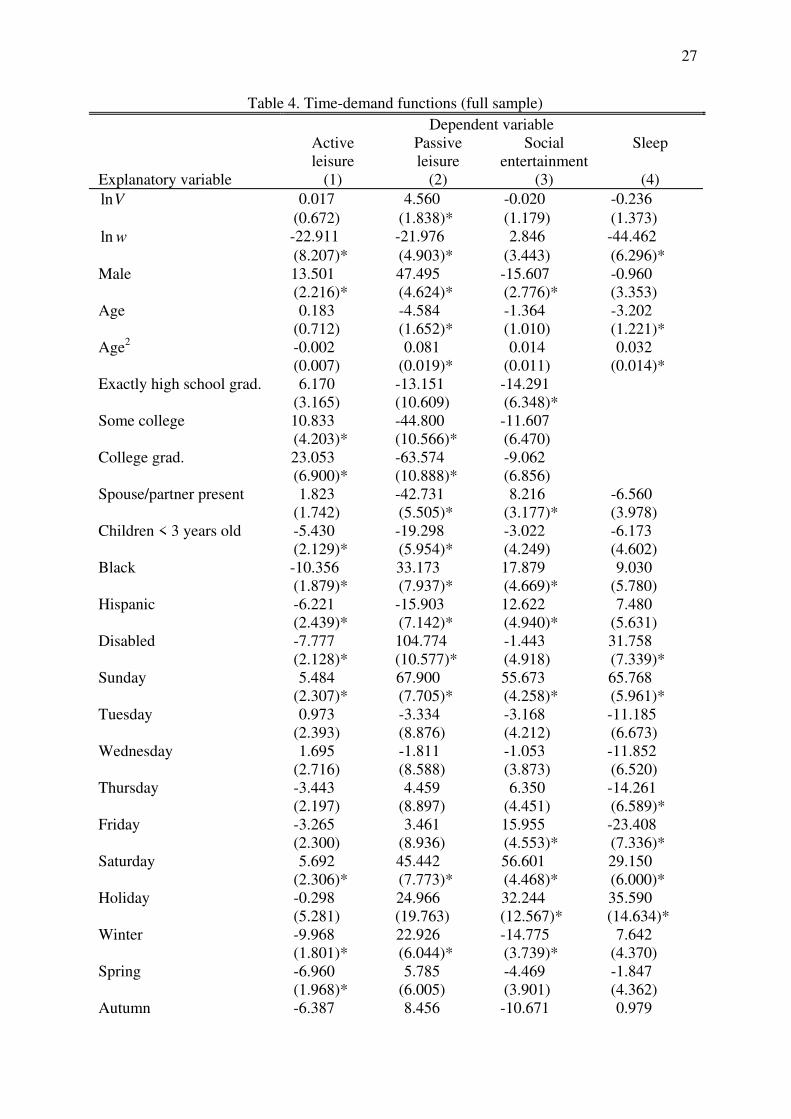
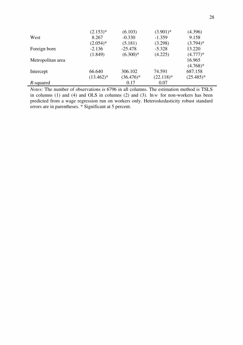
Table 4 presents the estimates of the time-demand regression functions obtained on the full
sample of men and women. In columns (1) and (4), pertaining, respectively, to active leisure
and sleep, TSLS estimates, which control for the endogeneity of ln w among workers, are
presented. The estimated coefficients in columns (2) and (3), which correspond to passive
leisure and social entertainment activities, are OLS estimates. In all the four regressions, ln w
for non-workers has been predicted from a wage regression run on workers only.
Heteroskedasticity robust standard errors are shown in parentheses.
The estimated income coefficient in the regressions for the three leisure aggregates is
generally small, attaining statistical significance at 0.05 level in the case of passive leisure
only. The implied income elasticity of this activity, calculated as the estimated coefficient
associated to lnV divided by the mean time devoted to passive leisure in the sample, is 0.021
(S.E. = 0.008), which suggests that passive leisure is a necessity. The implied reaction of
passive leisure to variations in income is such that, at average time allocation values, passive
leisure would increase by 2.1 percent (some 5 minutes per day) for a doubling of the income.
For sleep, the income coefficient is very small and does not attain statistical significance.
Overall, our results tend to agree with those found by Kooreman and Kapteyn (1987)
and Biddle and Hamermesh (1990) using the 1975-1976 TUS.9 They indicate that the effect
of income is generally unimportant, perhaps with the exception of passive leisure activities.
(Of course, this conclusion is compatible with the existence of very significant income effects
9 Findings, in particular, do not seem to be affected by the different design of the diary
instrument: The 1975-1976 TUS, while using a one-day diary format, obtained four time
diaries at three-month intervals from each respondent.
16
at a more disaggregated level, such as, for example, the many different sports comprised
within the active leisure aggregate.) However, for the same three leisure aggregates Dardis et
al. (1994) obtain expenditure elasticities for non-salary income in the range of 0.40 to 0.72,
which suggests that recreation goods and leisure time are not consumed in fixed proportion:
Ceteris paribus, an increase in income leads consumers to increase the goods intensity of
active leisure, passive leisure, and social entertainment. In other words, consumers opt to
increase the quality (understood as the amount of dollars spent per unit of time) of each of
those three leisure aggregates when endowed with more income. This conclusion is in line
with Gronau and Hamermesh’s (2006) findings on the effect of education and age (two
correlates of household income) on the relative goods intensity of leisure in the US and Israel.
Given the small income effects, the value of the coefficient associated to ln w will be
representing essentially a price-of-time effect on the demand for leisure/sleep. There are two
reasons why this price effect is expected to be negative, Becker (1965) argues: When the
wage rate is relatively high, consumers will economize on recreation, but they will also have
an incentive to economize on time and to spend more on goods in producing recreation. The
estimated wage effects on active leisure (-22.9), passive leisure (-22.0), and sleep (-44.5)
agree with this reasoning. Estimates are precise and attain statistical significance at 0.05 level.
At average time allocation values, the implied wage elasticities are, respectively, -1.30 (S.E. =
0.47), -0.10 (S.E. = 0.02), and -0.09 (S.E. = 0.01), which suggest that consumers will reduce
their weekly active leisure, passive leisure, and sleep by around 16, 15, and 33 minutes,
respectively, when offered a 10 percent increase in the wage rate. Our estimated sleep-wage
elasticity is substantially larger than that obtained by Biddle and Hamermesh (-0.04, S.E. =
0.02), which may be due to the different set of instruments for ln w utilized. The estimated
wage effect on social entertainment is positive but small, and does not attain statistical
17
significance. Instrumenting for ln w in the social entertainment equation yields an estimated
wage effect in the neighborhood of -10.0 (S.E. = 15.9).
Other significant effects are evident in Table 4. As expected, education exerts an
independent effect on the demand for active and passive leisure. What is perhaps surprising is
the magnitude of the effect: In comparison with a person who did not complete high school, a
college graduate spends on average some 23 minutes more per day in active leisure pursuits,
and some 64 minutes less in passive leisure activities. A consumer having a physical/mental
disability spends on average 105 minutes more per day on passive leisure, and sleeps 32
minutes more. Her active leisure activities, however, are curtailed by some 8 minutes per day,
but time spent on social entertainment is essentially unaffected. Living in the west region of
the US increases the time spent on active leisure by some 8 minutes per day. In comparison
with a native, a foreign born person sleeps 13 minutes more per day and spends some 25
minutes less in passive leisure on average. Residing in a metropolitan area has a substantial
positive effect on sleep duration (17.0, S.E. = 4.8).
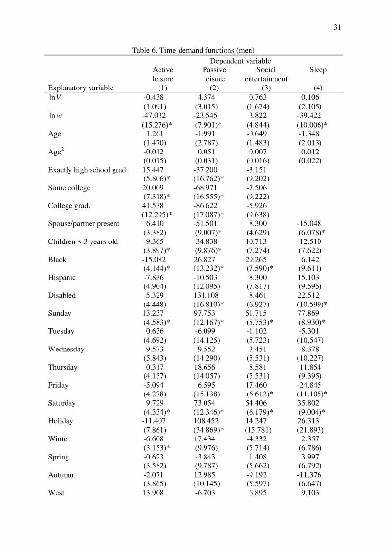
Tables 5 and 6 present the estimation output separately for women and men,
respectively. The estimated coefficients listed in Table 5 and in columns (2) and (3) of Table
6 are OLS estimates. Columns (1) and (4) of Table 6 present TSLS estimates, which control
for the endogeneity of ln w among workers. As in the full sample, ln w for non-workers has
been predicted from wage regressions (one for women and other for men) run on workers
only. To test for the equality of beta coefficients across sexes, I carry out tests of structural
break with unequal variances (e.g., see Greene, 2003). The null hypothesis is that
; ;j jx women x men
m m , where jx
m denotes the coefficient associated to
jx in the equation for
activity m . Assuming that the samples of men and women are independent, the robust t-
statistic
18
; ;
; ;
ˆ ˆ
ˆ ˆvar var
j j
j j
x women x men
m m
x women x men
m m
t
, (11)
where ̂ denotes either the OLS or the TSLS estimator and var is the corresponding
robust estimate of variance, has a limiting standard normal distribution under the null.
The estimated coefficients associated to lnV are generally small, not observing
significant differences between men and women. The wage effects on passive leisure and
social entertainment are also similar, but some differences are evident in the equations for
sleep and, especially, active leisure. The test of structural break does not reject the equality of
wage effects across sexes in the equation for sleep (p-value 0.10), but it does strongly reject
that restriction in the equation for active leisure (p-value 0.00). For women, a variation in the
wage rate holding other factors fixed leaves the time devoted to active leisure essentially
unchanged. For men, a 10 percent increase in the wage rate reduces their weekly active leisure
by some 33 minutes on average. The independent effect of education on active and passive
leisure discussed above derives essentially from men’s behavior. In the case of women, we
see no significant differences across educational categories in the time devoted to active
leisure pursuits. (Although for little margin, a test of the joint significance of the three
education dummies in the active leisure equation for women does not reject the null of no
significance, p-value 0.07). Similarly, we see that the increase in active leisure associated to
living in the West is essentially a male phenomenon: While a male living there spends some
14 minutes more per day on active leisure pursuits than a comparable male living in other
regions of the US, the implied effect for a female is an increase of about just 3 minutes.
5. CONCLUSION
There is evidence that the expenditure on goods consumed in the course of active leisure,
passive leisure, and social entertainment activities increases (moderately) with income.
However, we have found no evidence of income effects on the demand for time spent on
19
active leisure and social entertainment, and a very small positive reaction of passive leisure to
changes in income. We conclude, therefore, that the mix of recreation goods and leisure time
is not constant across income strata, as consumers endowed with more income opt to improve
the quality of their leisure activities but not to increase (or increase only slightly) the time
spent on them. As in Biddle and Hamermesh (1990), our estimated income elasticity of sleep
is not significantly different from zero.
Our estimated wage effects suggest that, at average time allocation values, consumers
will reduce their weekly passive leisure and sleep by around 15 and 33 minutes, respectively,
when offered a 10 percent increase in the wage rate. The same wage increase will have no
consequences for the demand of time spent on social entertainment, will leave women’s time
spent on active leisure activities essentially unaffected, but will induce men to reduce their
weekly active leisure by some 33 minutes on average. There is also evidence of a positive
direct effect of education on preferences for active leisure which derives essentially from
men’s behavior.
REFERENCES
Aguiar, Mark, and Erik Hurst. 2007. Measuring trends in leisure: The allocation of time over
five decades. The Quarterly Journal of Economics 122(3):969-1006.
Becker, Gary S. 1965. A theory of the allocation of time. The Economic Journal 75:493-517.
Biddle, Jeff, and Daniel Hamermesh. 1990. Sleep and the allocation of time. Journal of
Political Economy 98(5):922–943.
Blundell, Richard, and Thomas MaCurdy. 1999. Labor supply: a review of alternative
approaches. In Handbook of Labor Economics, vol. 3, ed. Orley Ashenfelter and
David Card. Amsterdam: Elsevier Science B. V.
20
Borjas, George J. 1999. The economic analysis of immigration. In Handbook of Labor
Economics, vol. 3, ed. Orley Ashenfelter and David Card. Amsterdam: Elsevier
Science B. V.
Dardis, Rachel, Horacio Soberon-Ferrer, and Dilip Patro. 1994. Analysis of leisure
expenditures in the United States. Journal of Leisure Research 26(4): 309-321.
Greene, William H. 1981. On the asymptotic bias of the Ordinary Least Squares estimator of
the Tobit model. Econometrica 49(2):505-513.
Greene, William H. 2003. Econometric Analysis, fifth edition. Pearson Education
International.
Gronau, Reuben. 1976. The allocation of time of Israeli women. Journal of Political Economy
84(4):S201-S220.
Gronau, Reuben, and Daniel S. Hamermesh. 2006. Time vs. goods: The value of measuring
household production technologies. Review of Income and Wealth 52(1):1-16.
Hamermesh, Daniel S., Harley Frazis, and Jay Stewart. 2005. Data watch. The American
Time Use Survey. Journal of Economic Perspectives 19(1):221-232.
Juster, F. Thomas, Paul Courant, Greg J. Duncan, John P. Robinson, and Frank P. Stafford.
1978. Time use in economic and social accounts, 1975-1976. Manuscript. Inter-
university Consortium for Political and Social Research. Ann Arbor, Michigan.
Kenkel, Donald S. 1991. Health behavior, health knowledge, and schooling. Journal of
Political Economy 99(2):287-305.
Kooreman, Peter, and Arie Kapteyn. 1987. A disaggregated analysis of the allocation of time
within the household. Journal of Political Economy 95(2):223-249.
21
McDonald, John F., and Robert A. Moffitt. 1980. The uses of Tobit Analysis. The Review of
Economics and Statistics 62(2): 318-321.
Mincer, Jacob. 1963. Market prices, opportunity costs, and income effects. In Measurement in
Economics: Studies in Mathematical Economics and Econometrics in Memory of
Yehuda Grunfeld, edited by C. Christ et al. Stanford, California: Stanford University
Press.
Mullahy, John and Stephanie A. Robert. 2010. No time to lose: Time constraints and physical
activity in the production of health. Review of Economics of the Household 4:409-
432.
Owen, John D. 1971. The demand for leisure. Journal of Political Economy 79(1):56-76.
Papke, L.E. and J.M. Wooldridge. 1996. Econometric methods for fractional response
variables with an application to 401 (K) plan participation rates. Journal of Applied
Econometrics 11(6): 619-632.
Sargan, J.D. 1958. The estimation of economic relationships using instrumental variables.
Econometrica 26:393-415.
Staiger, Douglas, and James H. Stock. 1997. Instrumental variables regression with weak
instruments. Econometrica 65(3):557-586.
Stapleton, David C., and Douglas J. Young. 1984. Censored normal regression with
measurement error on the dependent variable. Econometrica 52(3):737-760.
Stewart, Jay. 2013. Tobit or not Tobit? Journal of Economic and Social Measurement 38:263-
290.
Stoker, Thomas M. 1986. Consistent estimation of scaled coefficients. Econometrica
54(6):1461-1481.
22
Wales, T.J., and A.D. Woodland. 1977. Estimation of the allocation of time for work, leisure,
and housework. Econometrica 45(1):115-132.
Wooldridge, Jeffrey M. 2010. Econometric Analysis of Cross Section and Panel Data, second
edition. Cambridge, MA: The MIT Press.
23
Table 1. Sample descriptive statistics, the American Time Use Survey 2011
Variable (minutes) Mean SD Min Max % = 0
Women (3972 persons)
Active leisure 13.7 44.6 0 850 83.4
Passive leisure 198.6 180.8 0 1380 11.2
Social entertainment 72.1 117.2 0 1030 51.2
Sleep 524.5 131.8 0 1359 0.1
Men (2824 persons)
Active leisure 23.1 66.3 0 800 80.1
Passive leisure 243.1 210.4 0 1430 9.4
Social entertainment 57.9 108.8 0 1015 60.0
Sleep 514.2 134.4 0 1317 0.1
Variable Mean SD Min Max
Age 43.9 11.4 23 64
Annual nonlabor income (1000) 38.8 38.5 0.3 175.0
Average hourly earningsa 22.8 13.3 4.6 72.1
Years since migrationb 19.5 12.8 1 62.5
Variable (%) Mean Variable (%) Mean
Spouse/partner present 61.6 Winter 25.5
Children < 3 years old 13.8 Spring 25.0
Black 14.3 Summer 25.7
Hispanic 14.3 Autumn 23.8
Disabled 8.9 Less than high school graduate 8.5
Sunday 25.2 Exactly high school graduate 25.6
Monday 9.5 Some college 28.4
Tuesday 10.1 College graduate 37.5
Wednesday 10.4 Northeast 17.7
Thursday 10.1 Midwest 24.4
Friday 9.9 South 36.2
Saturday 24.8 West 21.7
Holiday 1.6 Metropolitan area 84.8
Foreign-born 17.0
Notes: Data are of 6796 persons aged 23-64 who are not self-employed. a: Workers only.