Some Internet Dynamics and Alternatives to TCP Friendly

Stephan Bohacek

University of Southern California

Joint work with: Boris Rozovskii, Joao Hespanha, Katia Obraczka, Junsoo Lee, Khusbboo Shah, Vinay Sridhara, and Raghava Sivaramu

Developing stochastic models of the Internet and investigating what can be

determined about the state of the Internet by observing round-trip times and drops.

Stephan Bohacek

University of Southern California

Joint work with: Boris Rozovskii, Joao Hespanha, Katia Obraczka, Junsoo Lee, Khusbboo Shah, Vinay Sridhara, and Raghava Sivaramu

preliminary work

Outline

• TCP friendly basics

• Problems with TCP – fixes

• Modeling RTT and estimating queue parameters

• Observed dynamics of queue model parameters

• Drop Model

• Observed dynamics of the drop model parameters

• An alternative to TCP friendly congestion control

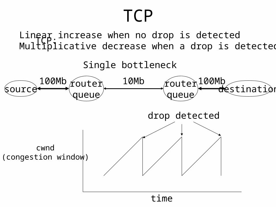
TCPLinear increase when no drop is detectedMultiplicative decrease when a drop is detected

TCP:

routerqueue

routerqueue

source destination100Mb 100Mb10Mb

Single bottleneck

cwnd(congestion window)

time

drop detected

Derivation of the TCP Friendly Rule

cwnd(congestion window)(number of packets

sent / RTT)

time

w*

w*/2 RTT – Roundtrip Time

Total number of packets sent between drops = w*/2 + w*/2+1+…+ w*/2 + w*/2 3/8 w*2

p := probability of a packet being dropped = 8/3 · 1/ w*2 (assumes one drop)

cwnd = ¾ w*

T := Sending Rate (pkts/sec) = cwnd (pkts/rtt) / RTT (sec/rtt)

T · RTT = cwnd = ¾ w*=(8/3)1/2 1/p1/2

T · RTT = C · 1/p1/2

not true

Similar formulas

T · RTT = C · 1/p1/2

C = 1.31 Ott, Kemperman and Mathis (1996)C = (8/3)1/2 Mathis, Semke, Mahdavi and Ott (1997)C = (3/2)1/2 Altman (2000) and others.C = 1.27 Hespanha, Bohacek, Obraczka and Lee 2001

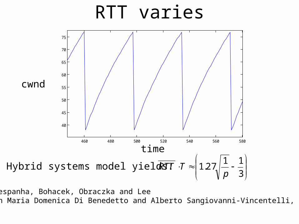
RTT varies

460 480 500 520 540 560 580

40

45

50

55

60

65

70

75

Hybrid systems model yields:

3

1127.1

pTRTT

Hespanha, Bohacek, Obraczka and Lee In Maria Domenica Di Benedetto and Alberto Sangiovanni-Vincentelli, Mar. 2001.

time

cwnd

Dumbbell topology

router router

S1

S2

S3

Sn

D1

D2

D3

Dn

Single bottleneck link

100Mbs

10Mbs

10-4

10-3

10-2

10-1

100

100

101

102

103

p - drop probability

RT

T *

T

The TCP Friendly Rule

Validation of the TCP Friendly Rule

RTT ·T = 1.02/p1/2

TCP performs poorly over multi-hop connections

router router router routersource destination

S1 D1 S2 Dn-1 DnSn

Competing TCP flows

p1 = dropprobability

pn = dropprobability

Each competing flow satisfies Ti · RTTi = C 1/pi1/2

Drop probability for multi-hop flow = 1 - i(1 - pi) >> pj

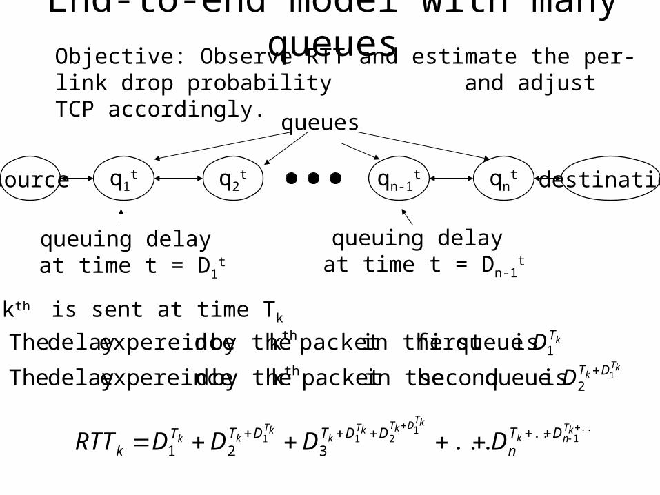
End-to-end model with many queuesObjective: Observe RTT and estimate the per-link drop probability

and adjust TCP accordingly.

q1t q2

t qn-1t qn

tsource destination

queues

queuing delay at time t = D1

t

queuing delay at time t = Dn-1

t

kTk DTD 1

2th is queue second in thepacket k by the dexpereincedelay The

kTD1th is queuefirst in thepacket k by the dexpereincedelay The

...1

1211 ...

321 ...

kT

nk

kTDkTkTk

kTkk DT

nDDTDTT

k DDDDRTT

The kth is sent at time Tk

Probability Density FittingMinimum Distance Fit

Invariant density of the delay experienced in M/M/1 queue (ignore increments)

p(Di = d) = p(d) = {d=0}(i - i) / i + (i - i) i /i exp(-(i - i)d)

i - departure rate at ith queuei - arrival rate at ith queue

Heavy-traffic assumptionAccount for most of the delay

p (d) i exp(-i d) for i i i

Minimum Distance Fit

dxxfxff

2

ˆˆmin

k

kNkobservedN

BRTTpBRTTp 2,

,min

Nipppp aN ***

21,

0for : xexp xi

i

i

non - convex optimization

Theoretical:

Actual:

where

convolution

RTT and Fitted Model 3/27/01LA – San Jose

Basic Queue Model

itqqq

iit dLdtdq ii

t max11 0

constant sending rate

random packet size

Poisson processwith intensity

indicator so 0 qi qimax – maximum queue size

Delay = Dit = qi

t /i

Distribution of Packet Sizes

0 0.1 0.2 0.3 0.4 0.5 0.6 0.7 0.8 0.9 10

0.1

0.2

0.3

0.4

0.5

0.6

0.7

0.8

0.9

1Cummulative Distribution of Normalized Packet Sizes

sz

Prob(Packet Size < sz) Minimum Packet Size = 0.0106 Prob(pkt size=1) = 0.09 Mean Packet Size=0.28

Measured 0.91 + 0.20 ln(sz)

Cumulative distribution of packet size. A packet of size one has 1500 bytes. The data was collected by the NLANR project.

Density function – (z)=0.2/z for 0.011 z 1

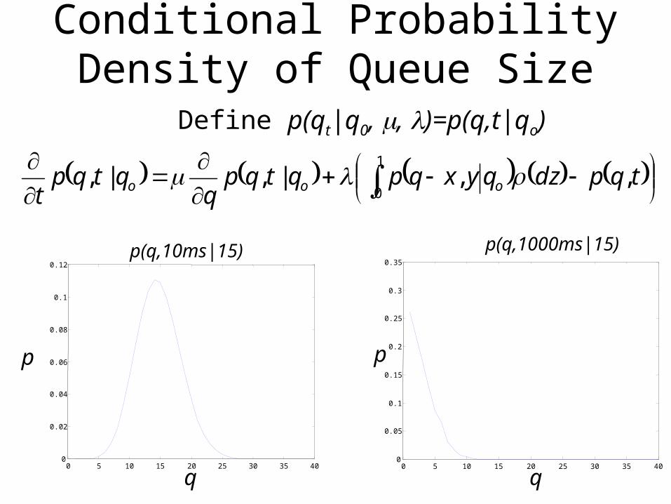
Conditional Probability Density of Queue Size

Define p(qt|q0, , )=p(q,t|qo)

0 5 10 15 20 25 30 35 400

0.02

0.04

0.06

0.08

0.1

0.12

0 5 10 15 20 25 30 35 400

0.05

0.1

0.15

0.2

0.25

0.3

0.35

tqpdzqyxqpqtqpq

qtqpt ooo ,,|,|,

1

0

p(q,10ms|15)

q q

p(q,1000ms|15)

p p

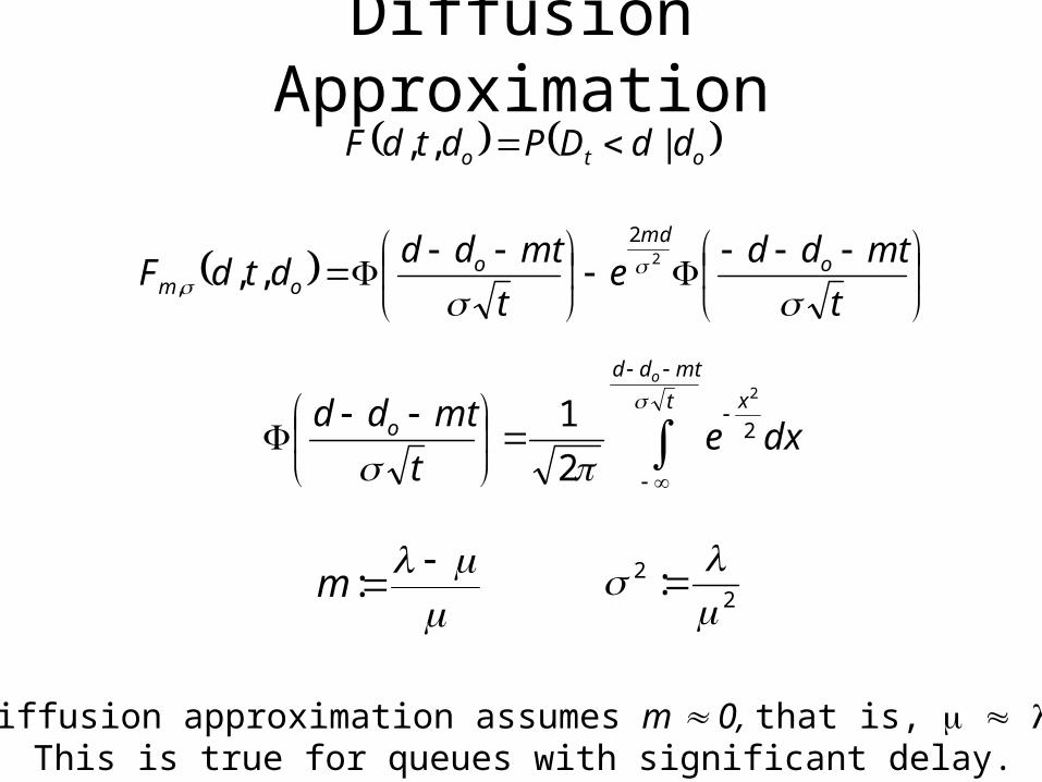
Diffusion Approximation oto ddDPdtdF |,,

t

mtdde

t

mtdddtdF o

md

oom

2

2

, ,,

t

mtdd

xo

o

dxet

mtdd

2

2

2

1

:m 2

2 :

Diffusion approximation assumes m 0, that is, . This is true for queues with significant delay.

Modification to the Diffusion Approximation

timework remaining to be processed

0 10 sec

1 sec 9 sec

P(d|t, do) = 0 for d< do - t

Two options1. Reflection 2. Accumulation

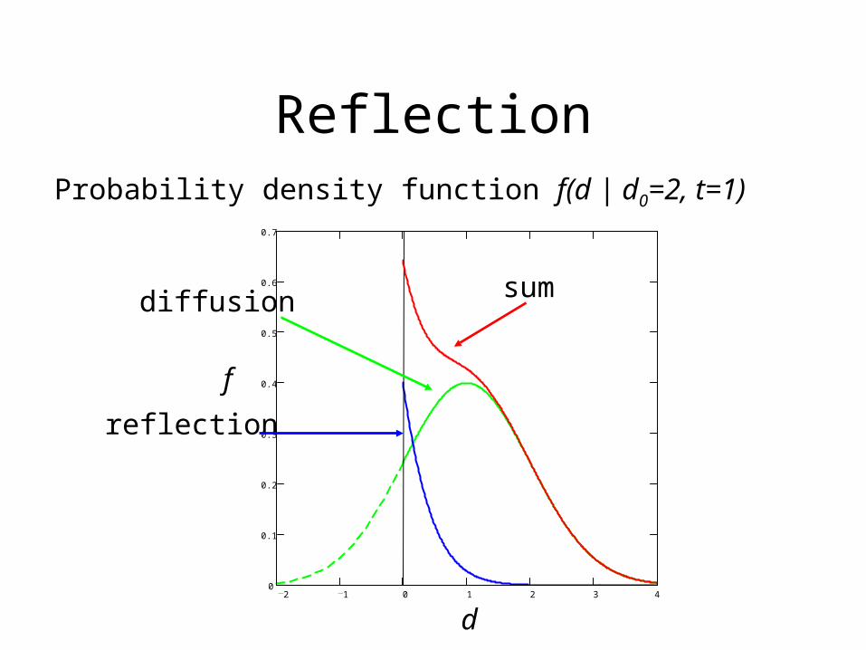
Reflection

2 1 0 1 2 3 40

0.1

0.2

0.3

0.4

0.5

0.6

0.7

diffusion

reflection

sum

Probability density function f(d | d0=2, t=1)

d

f

2 1 0 1 2 3 40

0.1

0.2

0.3

0.4

0.5

Accumulation

diffusion

Accumulate at d = do - t

Probability density function f(d | d0=2, t=1)

do - td

Modified Diffusion Approximation

oo dtdDPdtdF ,|,,

otherwise 0

for ,,2

2

,tdd

t

mtdde

t

mtdddtdF o

o

md

o

om

t

mtdd

xo

o

dxet

mtdd

2

2

2

1

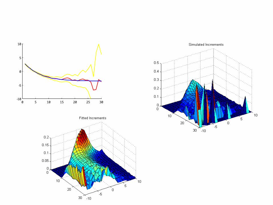
Histogram of Simulated RTT Increments

One Queue m0, <1t=10

Gaussian

One Queue m<<0, >>1t=10

Histogram of Simulated RTT Increments

Histogram of Simulated RTT Increments

Two Queues: Queue 1 – m1 << 0, 1 >> 1

Queue 2 – m20, 1 < 1

Histogram of Observed RTT Increments

Gaussian (RTT0=28)Queue empties slowly

Queue empties quickly

Estimating Parameters of the Diffusion Model

0 5 10 15 20 25 30-10

-5

0

5

10

Estimating Delay From RTT

Assume the kth drop occurs at t = tk

P( q1tk > qj

tk, j 1 | RTTK ) P( Queue 1 had the drop )

( Assumes that all queues are the same size )

P1k := P( D1

tk > Djtk, j 1 | RTTK ) P( Queue 1 had the drop )

( Assumes that all routers have the same speed )

Objective: Observe RTT and estimate the per-link drop probability and adjust TCP accordingly.

Adjusting TCP

p1 probability of queue 1 dropping a packet

p1 = k P1k / Total Number of Packets Sent

cwnd = T · RTT = C · mini (1/pi1/2)

Computing per Queue Drop Probabilities

KKKk

kK

kkK

k

DdRTTDpDg

DdRTTDpDgRTTDgE

|

||

n

DDDDDTTkkTDkTkT

kTDkTkTkTkkDDDDD

2

112

111 ,

321 ,,,,

Vector of delays experienced by the kth packet

nsobservatio RTT all of aggregate 1:: KkRTTRTTkt

K

,21

11

kTDkTkT DDkDg

delays queuing all of aggregate - 1:: KkDD kK

Computing per Queue Drop Probabilities

KKK

KKKk

KKKkk

DdRTTDp

DdRTTDpDg

DdRTTDpDgDgE

,

,

|

1,

K

tDRTT

KK DpRTTDpk

i

iktkt

211

||

KKKK tttt

K DDpDDpDp

Transition probabilities (we can compute these)

Computing per Queue Drop ProbabilitiesMonte-Carlo Markov Chain works, but is very slow.

i

kKKK

k iDgDdRTTDpDg

,

KkkK

k DdDdDdDdRTTDpDi

111, toaccording ddistribute is where

proposal density:

KlllK DDDDDD

,,,ˆ,,,ˆ

111

nl

ji

illll DDRTTDD ˆ,,ˆ,,ˆˆ 1

where j is random

il

il

il

il

il DDpDDpD 11 ||

2

1 toaccording ddistribute are ˆ

algorithm Metropolis -

ˆ,

,ˆˆ,1maxby given isy probabilit Acceptance

DDS

DDS

Dp

Dp

where l is random

0 5 10 15 20 25 30 35 40 45

0

5

10

15

20

25

30

35

Q1(k

)

Time

Size of Queue 1

0 50 100 150 200 250 300 350 400 4500

5

10

15

20

25

Time (ms)

RTT

Round Trip Time

0 10 20 30 40 500

2

4

6

8

10

12

14

16

18

20Size of Queue 2

Time

Q2(k)

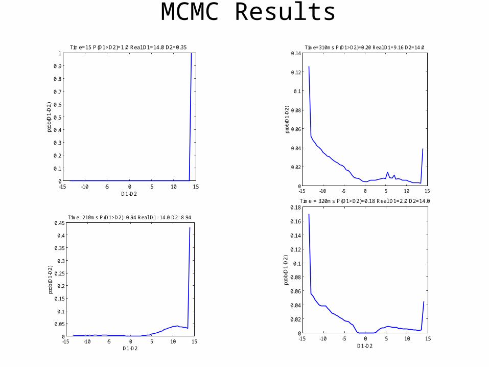
MCMC Results

-15 -10 -5 0 5 10 150

0.1

0.2

0.3

0.4

0.5

0.6

0.7

0.8

0.9

1Time=15 P(D1>D2)=1.0 Real D1=14.0 D2=0.35

D1-D2

prob

(D1-

D2)

-15 -10 -5 0 5 10 150

0.05

0.1

0.15

0.2

0.25

0.3

0.35

0.4

0.45Time=210ms P(D1>D2)=0.94 Real D1=14.0 D2=8.94

D1-D2

prob

(D1-

D2)

-15 -10 -5 0 5 10 150

0.02

0.04

0.06

0.08

0.1

0.12

0.14Time=310ms P(D1>D2)=0.20 Real D1=9.16 D2=14.0

D1-D2

prob

(D1-

D2)

-15 -10 -5 0 5 10 150

0.02

0.04

0.06

0.08

0.1

0.12

0.14

0.16

0.18Time = 320ms P(D1>D2)=0.18 Real D1=2.0 D2=14.0

D1-D2

prob

(D1-

D2)

0 50 100 150 200 250 3000

5

10

15

20

25Round Trip Time

Time (ms)

RTT

0 50 100 150 200 250 3000

2

4

6

8

10

12

14

16

18Delay in Queue 1

Time (ms)

D1

0 50 100 150 200 250 3000

2

4

6

8

10

12

14

16

18

20Delay in Queue 2

D2actual

expected

-15 -10 -5 0 5 10 150

0.05

0.1

0.15

0.2

0.25

0.3

0.35Time = 2 P(D1>D1)=0.25 Real D1=16.5 D2=0.48

D1 - D

2

Prob

-15 -10 -5 0 5 10 150

0.05

0.1

0.15

0.2

0.25

0.3

0.35

0.4Time = 4 P(D1>D1)=0.38 Real D1=15.0 D2=4.30

D1 - D

2

Prob

-15 -10 -5 0 5 10 150

0.01

0.02

0.03

0.04

0.05

0.06

0.07

0.08Time = 21 P(D1>D1)=0.69 Real D1=17.2 D2=8.86

D1 - D2

Prob

-15 -10 -5 0 5 10 150

0.02

0.04

0.06

0.08

0.1

0.12

0.14Time = 25 P(D1>D1)=0.01 Real D1=1.34 D2=12.0

D1 - D

2

Prob

-15 -10 -5 0 5 10 150

0.05

0.1

0.15

0.2

0.25

0.3

0.35Time = 2 P(D1>D1)=0.25 Real D1=16.5 D2=0.48

D1 - D

2

Prob

-15 -10 -5 0 5 10 150

0.05

0.1

0.15

0.2

0.25

0.3

0.35

0.4Time = 4 P(D1>D1)=0.38 Real D1=15.0 D2=4.30

D1 - D

2

Prob

-15 -10 -5 0 5 10 150

0.02

0.04

0.06

0.08

0.1

0.12

0.14Time = 25 P(D1>D1)=0.01 Real D1=1.34 D2=12.0

D1 - D2

Prob

-15 -10 -5 0 5 10 150

0.01

0.02

0.03

0.04

0.05

0.06

0.07

0.08Time = 20 P(D1>D1)=0.69 Real D1=17.2 D2=8.86

D1 - D

2

Prob

0 10 20 30 40 500

2

4

6

8

10

12

14Delay in Queue 1

Time (ms)

Prob

0 10 20 30 40 500

2

4

6

8

10

12

14Delay in Queue 2

Time (ms)

D2

0 50 100 150 200 250 300 350 400 4502

4

6

8

10

12

14

16

18

20Round Trip Time

Time (ms)

RTT

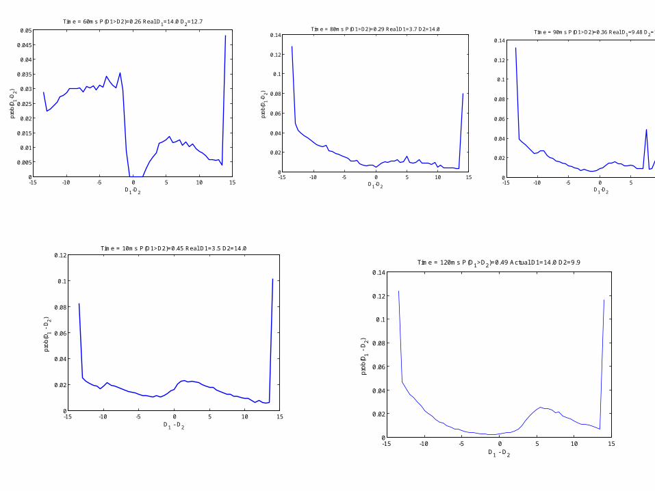
-15 -10 -5 0 5 10 150

0.005

0.01

0.015

0.02

0.025

0.03

0.035

0.04

0.045

0.05

Time = 60ms P(D1>D2)=0.26 Real D1=14.0 D

2=12.7

D1-D

2

pro

b(D

1-D2)

-15 -10 -5 0 5 10 150

0.02

0.04

0.06

0.08

0.1

0.12

0.14

Time = 90ms P(D1>D2)=0.36 Real D1=9.48 D

2=14.0

D1-D

2

pro

b(D

1-D2)

-15 -10 -5 0 5 10 150

0.02

0.04

0.06

0.08

0.1

0.12

0.14Time = 80ms P(D1>D2)=0.29 Real D1=3.7 D2=14.0

D1-D

2

pro

b(D

1-D2)

-15 -10 -5 0 5 10 150

0.02

0.04

0.06

0.08

0.1

0.12Time = 10ms P(D1>D2)=0.45 Real D1=3.5 D2=14.0

D1 - D

2

pro

b(D

1 - D

2)

-15 -10 -5 0 5 10 150

0.02

0.04

0.06

0.08

0.1

0.12

0.14

Time = 120ms P(D1>D

2)=0.49 Actual D1=14.0 D2=9.9

D1 - D

2

pro

b(D

1 - D

2)

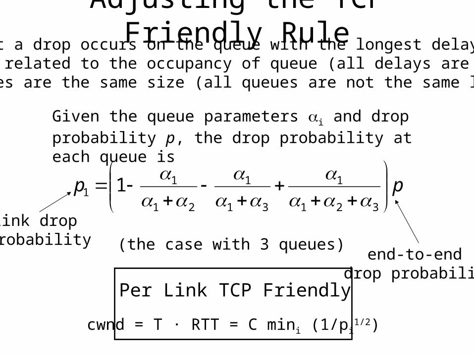
Adjusting the TCP Friendly Rule

Given the queue parameters i and drop probability p, the drop probability at each queue is

pp

321

1

31

1

21

11 1

(the case with 3 queues)end-to-end

drop probability

link drop probability

Assume that a drop occurs on the queue with the longest delay.- Delay is related to the occupancy of queue (all delays are not equal).- All queues are the same size (all queues are not the same length).

cwnd = T · RTT = C mini (1/pi1/2)

Per Link TCP Friendly

Observed Dynamics of the Queue Parameters

RTTt = i Dt

i

p(Dti = d ) = i exp( - i d ) for d 0

E(Dti) = 1/ i - The smaller the i the more significant the queue.

00

0.5

1

1.5

2

2.5

3

3.5

4

4.5

5

Monday Tuesday Wednesday Thursday Friday Saturday Sunday Monday

Time Series of the Smallest Queue Parameter

00

1

2

3

4

5

6

7

8

9

10

Monday Tuesday Wednesday Thursday Friday Saturday Sunday Monday

Time Series of the Next to Smallest Queue Parameter

00

0.5

1

1.5

2

2.5

3

3.5

4

4.5

5

Monday Tuesday Wednesday Thursday Friday Saturday Sunday Monday

Slightly Smoothed Time Series of the Smallest Queue Parameter

00

1

2

3

4

5

6

7

Monday Tuesday Wednesday Thursday Friday Saturday Sunday Monday

Slightly Smoothed Time Series of the Next to Smallest Queue Parameter

0 10 20 30 40 50 60 70 80 90 100-0.15

-0.1

-0.05

0

0.05

0.1

0.15

0.2

0.25

0.3

0.35Autocorrelation of Increments of the Smallest Queue Parameter

The autocorrelation decays very quickly,

hence a low order model should suffice (maybe even a Markov chain).

Autocorrelation of the increments of the smallest queue parameter.

0 10 20 30 40 50 60 70 80 90 100-0.4

-0.2

0

0.2

0.4

0.6

0.8

1

1.2

1.4

1.6Autocorrelation of Increments of the Next to Smallest Queue Parameter

smallest parameter

next to smallest parameter

Transition Probabilities Matrix

1

1

Transition Probabilities for the Smallest Queue Parameter0

00.5

0.5

1

1

1.5

1.5

2

2

2.5

2.5

3

3

3.5

3.5

4

4

4.5

4.5

5

5

1

1

Transition Probabilities for the Next to Smallest Queue Parameter0

00.5

0.5

1

1

1.5

1.5

2

2

2.5

2.5

3

3

3.5

3.5

4

4

4.5

4.5

5

5

Smallest Queue Parameter Next to Smallest Queue Parameter

Pi,j P|i-j|

The transition probability are nearly spatially homogeneous

Partition the parameter space and estimate transition probabilities

-3 -2 -1 0 1 2 30

0.05

0.1

0.15

0.2

0.25

0.3

0.35 Distribution of the Next to Smallest Queue Parameter Increments

-3 -2 -1 0 1 2 30

0.05

0.1

0.15

0.2

0.25

0.3

0.35Distribution of the Smallest Queue Parameter Increments

Transition Probability

Size of Increment Size of Increment

prob

abili

ty

prob

abili

ty

Smallest Queue Parameter Next to Smallest Queue Parameter

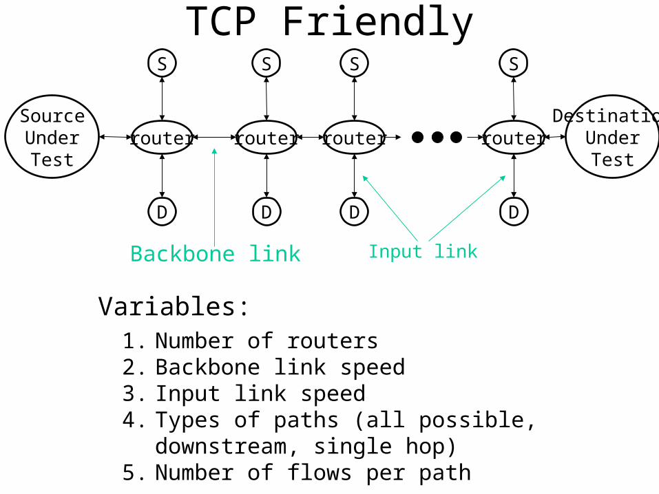
TCP Friendly

router

S

D

router

S

D

router

S

D

router

S

D

SourceUnderTest

DestinationUnderTest

Backbone link Input link

Variables:1. Number of routers2. Backbone link speed3. Input link speed4. Types of paths (all possible, downstream, single hop)5. Number of flows per path

The TCP Friendly Rule

It is possible that topologies that never exists were considered.It is possible that worst topologies exists that have yet to be considered.Further study is under way.

Time-Varying TCP Friendly

0 50 100 150 200 250 3000

0.1

0.2

0.3

0.4

0.5

0.6

0.7

0.8Time Varying TCP Friendly Relationship

RT

T *

T *

p1/

2

Seconds

cwnd = T · RTT = C mini (1/pi1/2)

Even if the TCP rule is accurate, it is not clear how to compute RTT, p, T.

Alternatives to the TCP Friendly Rule(TCP Mimicking)

tt

tt dN

Xdt

RTTdX

2

1

Very simple continuous time model of TCP

Xt := window sizeNt := drop process

RTTt := roundtrip time

Approach: 1. Observe RTT and drops.2. Determine the pdf of TCP’s window size.

At what rate would a TCP flow send data if it was in the same situation?

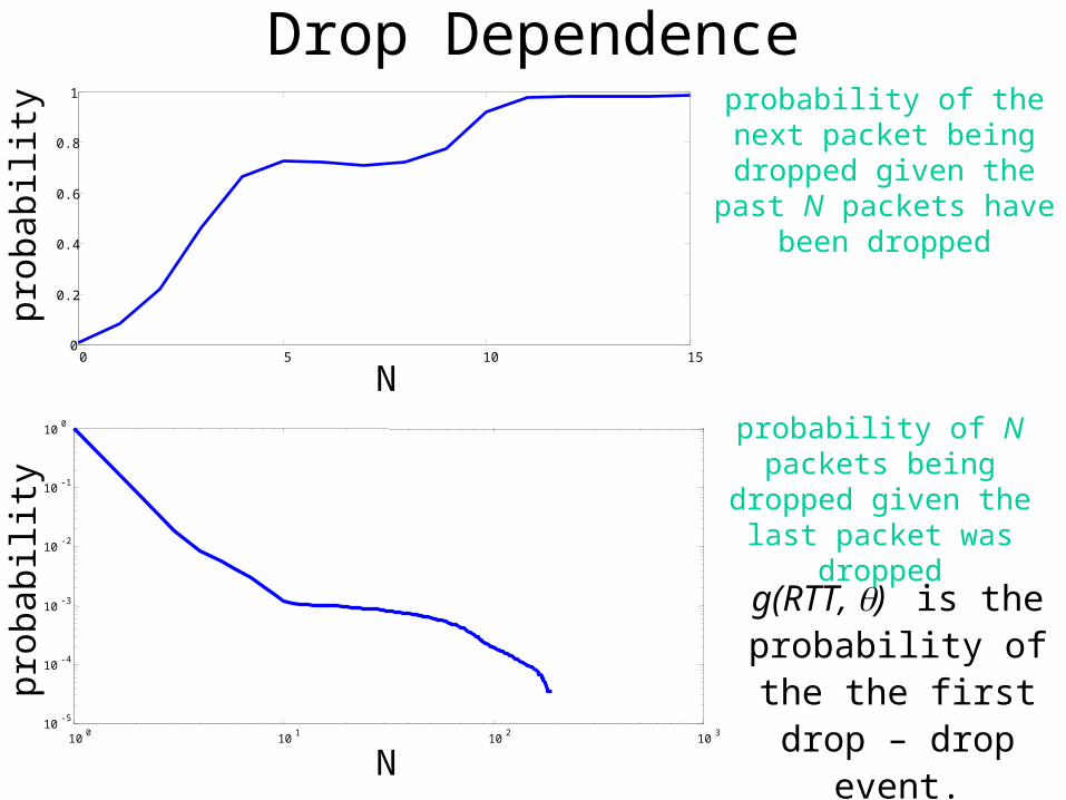
Drop Models• Ott (1997) considered deterministic drops.• Padhye (1998) assumed drops to be highly correlated over short

time scales, but independent over longer time scales.• Altman (2000) assumes drops are bursty.• Altman (2000) drop events are modeled as renewal processes with

particular examples, deterministic, Poisson, i.i.d., and Markovian.• Savari (1999) drop events are modeled as Poisson where the

intensity depends on the window size of the TCP protocol.

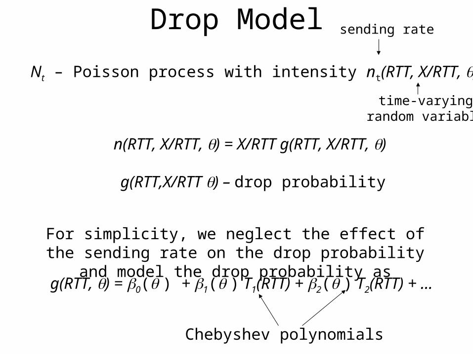
Drop Model

Nt – Poisson process with intensity nt(RTT, X/RTT, )

n(RTT, X/RTT, ) = X/RTT g(RTT, X/RTT, )

g(RTT,X/RTT ) – drop probability

time-varyingrandom variable

sending rate

g(RTT, ) = 0( ) + 1( ) T1(RTT) + 2( ) T2(RTT) + …

Chebyshev polynomials

For simplicity, we neglect the effect of the sending rate on the drop probability and model the drop probability as

Drop Dependence

0 5 10 150

0.2

0.4

0.6

0.8

1 probability of the next packet being dropped given the past N packets have been

dropped

prob

abil

ity

N

100

101

102

103

10-5

10-4

10-3

10-2

10-1

100 probability of N packets

being dropped given the last packet was dropped

N

prob

abil

ity

g(RTT, ) is the probability of the the

first drop – drop event.

Drop – Event Probability

Drop Model Parameter Variation

1

5

10

15

x 10-3 Drop Model Parameter Variation

X 1

1

0

10

20x 10

-3

X 2

1-20

-10

0

x 10-3

X 3

1-10

-50

5

x 10-3

Monday Tuesday Wednesday Thursday Friday Saturday Sunday

X 4

g(RTT, ) = 0( ) + 1( ) T1(RTT) + 2( ) T2(RTT) + …

0

05

1015

x 10-8

E(X

1(t) X

1(t+ )

)

Autocorrelation of the Drop Model Parameters

0

0123

x 10-7

E(X

2(t) X

2(t+ )

)

0

05

1015

x 10-8

E(X

3(t) X

3(t+ )

)

0

0

2

4x 10

-7

E(X

4(t) X

4(t+ )

)

1 2 3 hours

Autocorrelation of the Drop Models Parameters

There appears to be some correlation, but …

Transition Probability for Drop Model Parameter

1

1

Transition Probabilities for X10.000

0.0000.007

0.007

0.014

0.014

0.020

0.020

0.027

0.027

0.034

0.034

0.041

0.041

0.047

0.047

0.054

0.054

0.061

0.061

0.068

0.068

tt

tt dN

Xdt

RTTdX

2

1

At what rate would a TCP flow send data if it was in the same situation?

Alternatives to the TCP Friendly Rule(TCP Mimicking)

i

iit

i

itt qDRTT /

itqqq

iit dLdtdq ii

t max11 0

it rate with processPoission - iL

Tmatrix intensity with Process Markov -

ii matrix intensity with Process Markov -

, ,/ rate with processPoission - RTTRTTXnN i

Alternatives to the TCP Friendly Rule(single queue)

functiondensity y probabilit thebe to,,,, Define ttt qxp

,,,,:,,,, ttttt qxpqxp

,,,,,,,,

,,,,,,,,

,/,/

2,,,,

,/,/

2,,,,22

,,,,,,,,/

1,,,,

,, jqxpjqxpT

qxpdzzzqxp

TqTq

xnqxp

TqTq

xnqxp

qxpq

qxpxTq

qxpt

tj

jtj

j

tt

pp

t

pp

t

ttp

t

TCP Mimicking

• Every time an ack arrives and every time a packet is about to be sent, the pdf is evaluated.

• The decision whether to send a packet is based on the pdf and on the application, e.g. multimedia v.s. file transfer.

• If acks fail to arrive, the drop probability quickly adjusts to indicate that a TCP flow would send at a slow rate (unlike other rate based congestion control).

• It is not clear if TCP mimicking leads to TCP friendly.

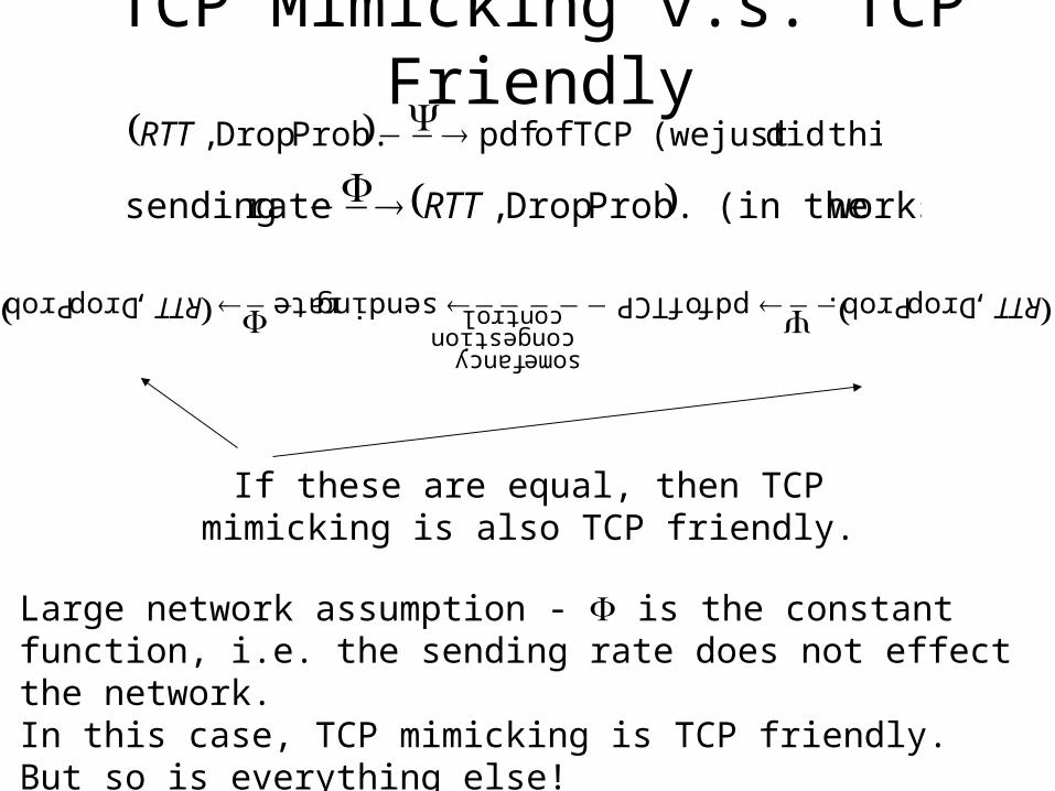
TCP Mimicking v.s. TCP Friendly this)didjust (we TCP of pdfProb. Drop , RTT

works)(in the Prob. Drop , rate sending RTT

Prob. Drop , rate sending TCP of pdf Prob. Drop ,control congestion

fancy some

RTT RTT If these are equal, then TCP mimicking is also

TCP friendly.

Large network assumption - is the constant function, i.e. the sending rate does not effect the network.In this case, TCP mimicking is TCP friendly. But so is everything else!

Future Work

• More of the same – more data, diversity paths. More data for drops during large RTT.

• Large network assumption – I/O dynamics (in progress)

• Determine qmax from data – relating RTT and queue model parameters to drop model parameters.

Conclusions

• It appears possible to develop stochastic models of the internet.• It appears possible the estimate parameters and the state of the

Internet from the observations, RTT and drops.• These models and estimation techniques may be useful in

developing congestion control algorithms.

The end