Some Mathematical and Numerical Issues in ...fluid/paper/73.pdf · Some Mathematical and Numerical...

COMMUNICATIONS IN COMPUTATIONAL PHYSICSVol. 3, No. 4, pp. 759-793

Commun. Comput. Phys.April 2008

REVIEW ARTICLE

Some Mathematical and Numerical Issues in

Geophysical Fluid Dynamics and Climate Dynamics

Jianping Li1 and Shouhong Wang2,∗

1 State Key Laboratory of Numerical Modeling for Atmospheric Sciences andGeophysical Fluid Dynamics (LASG), Institute of Atmospheric Physics (IAP),Chinese Academy of Sciences (CAS), P.O. Box 9804, Beijing 100029, China.2 Department of Mathematics, Indiana University, Bloomington, IN 47405, USA.

Received 11 January 2007; Accepted (in revised version) 10 November 2007

Communicated by Jie Shen

Available online 11 December 2007

Abstract. In this article, we address both recent advances and open questions in somemathematical and computational issues in geophysical fluid dynamics (GFD) and cli-mate dynamics. The main focus is on 1) the primitive equations (PEs) models and theirrelated mathematical and computational issues, 2) climate variability, predictabilityand successive bifurcation, and 3) a new dynamical systems theory and its applica-tions to GFD and climate dynamics.

AMS subject classifications: 86A05, 86A10, 76D, 76E, 76U05, 37L, 37M20, 35Q, 65

Key words: Geophysical fluid dynamics, climate dynamics, low-frequency variability, attractorbifurcation, dynamic transition, well-posedness.

Contents

1 Introduction 7602 Modeling 7613 Some theoretical and computational issues for the PEs 7654 Nonlinear error growth dynamics and predictability 7715 Climate variability and successive bifurcation 7746 New dynamical systems theories and geophysical applications 777

∗Corresponding author. Email addresses: [email protected] (J. P. Li), [email protected] (S. H. Wang)

http://www.global-sci.com/ 759 c©2008 Global-Science Press

760 J. P. Li and S. H. Wang / Commun. Comput. Phys., 3 (2008), pp. 759-793

1 Introduction

The atmosphere and ocean around the earth are rotating geophysical fluids, which arealso two important components of the climate system. The phenomena of the atmosphereand ocean are extremely rich in their organization and complexity, and a lot of them can-not be produced by laboratory experiments. The atmosphere or the ocean or the coupleatmosphere and ocean can be viewed as an initial and boundary value problem (Bjerk-nes [5], Rossby [125], Phillips [120]), or an infinite dimensional dynamical system. Thesephenomena involve a broad range of temporal and spatial scales (Charney [11]). For ex-ample, according to J. von Neumann [147], the motion of the atmosphere can be dividedinto three categories depending on the time scale of the prediction. They are motions cor-responding respectively to the short time, medium range and long term behavior of theatmosphere. The understanding of these complicated and scientific issues necessitate ajoint effort of scientists in many fields. Also, as John von Neumann [147] pointed out, thisdifficult problem involves a combination of modeling, mathematical theory and scientificcomputing.

In this article, we shall address mathematical and numerical issues in geophysicalfluid dynamics and climate dynamics. The main topics include:

1. issues on the modeling, mathematical analysis and numerical analysis of the prim-itive equation (PEs),

2. climate variability, predictability and successive bifurcation,

3. a new dynamical systems theory and its applications to geophysical fluid dynamics.

As we know, the atmosphere is a compressible fluid and the seawater is a slightlycompressible fluid. The governing equations for either the atmosphere, or the ocean, orthe coupled atmosphere-ocean models are the general equations of hydrodynamic equa-tions together with other conservation laws for such quantities as the energy, humidityand salinity, and with proper boundary and interface conditions. Most general circula-tion models (GCMs) are based on the PEs, which are derived using the hydrostatic as-sumption in the vertical direction. This assumption is due to the smallness of the aspectratio (between the vertical and horizontal length scales). We shall present a brief surveyon recent theoretical and computational developments and future studies of the PEs.

One of the primary goals in climate dynamics is to document, through careful theo-retical and numerical studies, the presence of climate low frequency variability, to verifythe robustness of this variability’s characteristics to changes in model parameters, andto help explain its physical mechanisms. The thorough understanding of this variabilityis a challenging problem with important practical implications for geophysical efforts toquantify predictability, analyze error growth in dynamical models, and develop efficientforecast methods. As examples, we discuss a few sources of variability, including wind-driven (horizontal) and thermohaline (vertical) circulations, El Nino-Southern Oscillation(ENSO), and Intraseasonal oscillations (ISO).

J. P. Li and S. H. Wang / Commun. Comput. Phys., 3 (2008), pp. 759-793 761

The study of the above geophysical problems involves on the one hand applicationsof the existing mathematical and computational theories to the understanding of the un-derlying physical problems, and on the other hand the development of new mathematicaltheories.

We shall present briefly a dynamic bifurcation and stability theory and its applica-tions to GFD. This theory, developed recently by Ma and Wang [100], is for both finiteand infinite dimensional dynamical systems, and is centered at a new notion of bifur-cation, called attractor bifurcation. The theory is briefly described by a simple systemof two ordinary differential equations, and by the classical Rayleigh-Benard convection.Applications to the stratified Boussinesq equations model and the doubly-diffusive mod-els are also addressed.

We would like to mention that there are many important issues not covered in thisarticle, including, for example, the ocean and atmosphere data assimilation and predic-tion problems, and the stochastic-dynamics studies; see, among many others, [20, 30, 31,33, 34, 38, 39, 56, 60–64, 108] and the references therein.

The article is organized as follows. In Section 2, some basic GFD models are intro-duced, with some mathematical and computational issues given in Section 3. Section 4 ison predictability, and Section 5 deals with issues on climate variability. Section 6 presentsthe new dynamical systems theory based on attractor bifurcation and its application toRayleigh-Benard convection and to GFD models.

2 Modeling

2.1 The primitive equations (PEs) of the atmosphere

Physical laws governing the motion and states of the atmosphere and ocean can be de-scribed by the general equations of hydrodynamics and thermodynamics. Using a non-inertial coordinate system rotating with the earth, these equations can be written as fol-lows:

∂~V

∂t+~V ·∇3~V+2~Ω×~V−~g+

1

ρgrad3p= ~DM,

∂ρ

∂t+div3(ρ~V)=0,

cv∂T

∂t+cv~V ·∇3T+

p

ρ∇3~V =Q+DH,

∂q

∂t+~V ·∇3q=

S

ρ+Dq,

p= RρT.

(2.1)

Here the first equation is the momentum equation, the second is the continuity equation,the third is the first law of thermodynamics, the fourth is the diffusion equation for thehumidity, and the last is the equation of state for an ideal gas. The unknown functions


are the three-dimensional velocity field ~V, the density function ρ, the pressure function p,the temperature function T, and the specific humidity function q. Moreover, in the above

equations, ~Ω stands for the angular velocity of the earth,~g the gravity, R the gas constant,cv the specific heat at constant volume, ~DM the viscosity terms, DH the temperature dif-fusion, Q the heat flux per unit density at the unit time interval, which includes moleculeor turbulent, radiative and evaporative heating, and S the differences of the rates of theevaporation and condensation.

These equations are normally far too complicated; simplifications from both the phys-ical and mathematical points of view are necessary. There are essentially two characteris-tics of both the atmosphere and ocean, which are used in simplifying the equations. Thefirst one is that for large scale geophysical flows, the ratio between the vertical and hor-izontal scales is very small; this leads to the primitive equations (PEs) of both the atmo-sphere and the ocean, which are the basic equations for these two fluids. More precisely,the PEs are obtained from the general equations of hydrodynamics and thermodynam-ics of the compressible atmosphere, by approximating the momentum equation in thevertical direction with the hydrostatic equation:

∂p

∂z=−ρg. (2.2)

This hydrostatic equation is based on the ratio between the vertical and horizontal scalebeing small. Here ρ is the density, g the gravitational constant, and z= r−a height abovethe sea level, r the radial distance, and a the mean radius of the earth. Equation (2.2)expresses the fact that p is a decreasing function along the vertical so that one can use pinstead of z as the vertical variable. Motivated by this hydrostatic approximation, we canintroduce a generalized vertical coordinate system s-system given by

s= s(θ,ϕ,z,t), (2.3)

where s is a strict monotonic function of z. Then the basic equations of the large-scaleatmospheric motion in the s-system are

∂v

∂t+v·∇sv+ s

∂v

∂s+ f k×v+

1

ρ∇sz= DM,

∂p

∂s

∂s

∂z+ρg=0,

∂

∂s

(

∂p

∂t

)

s

+∇s ·(

v∂p

∂s

)

+∂

∂s

(

s∂p

∂s

)

=0,

cv∂T

∂t+cvv·∇sT+cv s

∂T

∂s+

1

ρ

(

∂p

∂t+v·∇s p+ s

∂p

∂s

)

=Q+DH,

∂q

∂t+v·∇sq+ s

∂q

∂s=

S

ρ+Dq.

(2.4)


Some common s-systems in meteorology are respectively the p-system (the pressure coor-dinate), the σ-system (the transformed pressure coordinate), the θ-system (the isentropiccoordinate), and the ζ-system (the topographic coordinate or transformed height coordi-nate). The above PEs appear in the literature in e.g. the books of A. E. Gill [42], G. Haltinerand R. Williams [43], J. R. Holten [44], J. Pedlosky [118], J. P. Peixoto and A. H. Oort [119],W. M. Washington and C. L. Parkinson [152], Q. C. Zeng [159]. We remark here thatsometimes the pressure coordinate is denoted by η, and the terrain-following by σ.

For simplicity, here we discuss only the case with the coordinate transformation from(θ,ϕ,z) to (θ,ϕ,p). The basic equations of the atmosphere are then the Primitive Equations(PEs) of the atmosphere in the p-coordinate system. As they appear in classical meteorol-ogy books (see e.g. [159] and Salby [128]), the PEs are given by

∂v

∂t+v·∇v+ω

∂v

∂p+2Ωcosθk×v+∇Φ= DM ,

∂Φ

∂p+

RT

p=0,

div v+∂ω

∂p=0,

∂T

∂t+v·∇T+ω

(

κT

p− ∂T

∂p

)

=Qrad

cp+

Qcon

cp+DH,

∂q

∂t+v·∇q+ω

∂q

∂p=E−C+Dq,

(2.5)

where DM is the dissipation term for momentum and DH and Dq are diffusion terms forheat and moisture, respectively, E and C are the rates of evaporation and condensationdue to cloud processes, cp the heat capacity, and Qrad and Qcon the net radiative heatingand the heating due to condensation processes, respectively. We use the pressure coordi-nate system (θ,ϕ,p), where θ (0<θ<π) and ϕ (0<ϕ<2π) are the colatitude and longitudevariables, and p the pressure of the air. The nondynamical processes Qrad, Qcon, E andC are called model physics. Furthermore, the unknown functions are the horizontal ve-locity v, the vertical velocity ω = dp/dt, the geopotential Φ, the temperature T, and thespecific humidity q. The operators div and ∇ are the two dimensional operators on thesphere.

Of course, this set of equations is supplemented with a set of physically sound bound-ary conditions such as (3.3), depending on the specific form of the forcing and dissipation.

2.2 Ocean models

The sea water is almost an incompressible fluid, leading to the Boussinesq approxima-tion, i.e., a variable density is only recognized in the buoyancy term and the equation of


state. The resulting equations are called the Boussinesq equations given as follows:

∂v

∂t+∇vv+w

∂v

∂z+

1

ρ0gradρ+ f k×v−µv−ν

∂2 v

∂z2=0,

∂w

∂t+∇vw+w

∂w

∂z+

1

ρ0

∂ρ

∂z+

ρ

ρ0g−µw−ν

∂2w

∂z2=0,

divv+∂w

∂z=0,

∂T

∂t+∇vT+w

∂T

∂z−µTT−νT

∂2T

∂z2=0,

∂S

∂t+∇vS+w

∂S

∂z−µSS−νS

∂2S

∂z2=0,

ρ=ρ0(1−βT(T−T0)+βS(S−S0)),

(2.6)

where v is the horizontal velocity field, w the vertical velocity, and S the salinity. Thesixth equation in (2.6) is an empirical equation for the density function based on thelinear approximation. In general, density ρ is a nonlinear function of T, S, and p. Withhigher approximations, one will encounter additional mathematical difficulties althoughthe nonlinear equation of state is essential for some elements of ocean circulation (e.g.,cabbeling).

As in the atmospheric case, the hydrostatic assumption is usually used, leading to thePEs for the large-scale ocean:

∂v

∂t+∇vv+w

∂v

∂z+

1

ρ0∇p+ f k×v−µv∆av−νv

∂2v

∂z2=0,

∂p

∂z=−ρg,

div v+∂w

∂z=0,

∂T

∂t+∇vT+w

∂T

∂z−µT∆aT−νT

∂2T

∂z2=0,

∂S

∂t+∇vS+w

∂S

∂z−µs∆aS−ν

∂2S

∂z2=0,

ρ=ρ0(1−βT(T−T0)+βS(S−S0)).

(2.7)

Also, we note that if the hydrostatic assumption is made first, the Boussinesq approxi-mation is not really necessary (see e.g. (2.5) – divergence-free! – or, e.g., de Szoeke andSamelson [19].

2.3 Coupled atmosphere-ocean models

Coupled atmosphere and ocean models consist of 1) models for the atmosphere compo-nent, 2) models for the ocean component, and 3) interface conditions. The interface con-


ditions are used to couple the atmosphere and ocean systems, and are usually derivedbased on first principles; see Gill [42], Washington and Parkinson [152]. A mathemati-cally well-posed coupled model with physically sound interface conditions and the PEsof the atmosphere and the ocean are given in Lions, Temam and Wang [85]. We referinterested readers to these references for further studies.

As we know, the atmosphere and ocean components have quite different time scales,leading to complicated dynamics. For example, from the computational point of view,one needs to incorporate the two time scales; see e.g. [88].

3 Some theoretical and computational issues for the PEs

3.1 Dynamical systems perspective of the models

From the mathematical point of view, we can put the models addressed in the previoussection in the perspective of infinite-dimensional dynamical systems as follows:

ϕt+Aϕ+R(ϕ)= F,

ϕ|t=0 = ϕ0,(3.1)

defined on an infinite-dimensional phase space H. Here A:H→H is an unbounded linearoperator, R : H→H is a nonlinear operator, F is the forcing term, and ϕ0 is the initial data.

We remark here that the linear operator can usually be written as A= A1+A2, whereA1 stands for the irreversible diabatic linear processes of energy dissipation, and A2 forthe reversible adiabatic linear processes of energy conversation. The nonlinear term R(ϕ)represents the reversible adiabatic nonlinear processes of energy conversation. The prop-erties of these operators reflect directly the essential characteristics of two kinds of basicprocesses with entirely different physical meanings.

The above formulation is often achieved by (a) establishing a proper functional settingof the model, and (b) proving the existence and uniqueness of the solutions.

Hereafter we demonstrate the procedure with the PEs. Due to some technical reasons,some minor and physically reasonable modifications of the PEs are made. In particular,we assume that the model physics Qrad, Qcon, E and C are given functions of location andtime. We specify also the viscosity, diffusion terms as (see among others Lions et al. [83]and Chou [16]):

DM =−L1v,

Qrad

cp+

Qcon

cp+DH =−L2T+QT,

E−C+Dq =−L3q+Qq,

Li =−µi∆−νi∂

∂p

(

(

gp

RT(p)

)2 ∂

∂p

)

,

(3.2)


where µi,νi are horizontal and vertical viscosity and diffusion coefficients, ∆ is the Laplaceoperator on the sphere, QT and Qq are treated as given functions, and T(p) a given tem-perature profile, which can be considered as the climate average of T. The boundaryconditions for the PEs are given by

∂

∂p(v,T,q)=(γs(vs−v), αs(Ts−T), αq(qs−q)), ω =0 at p= P,

∂

∂p(v,T,q)=0, ω =0 at p= p0.

(3.3)

The second and third equations (2.5) are diagnostic ones; integrating them in p-direction,we obtain

∫ P

p0

div v(p′)dp′ =0,

ω =W(v)=−∫ p

p0

div v(p′)dp′ ,

Φ=Φs +∫ P

p

RT(p′)p′

dp′.

(3.4)

Then the PEs are equivalent to the following functional formulation:

∂u

∂t+Λ(v)u+P(u)+Lu+(∇Φs,0,0)=(0,QT ,Qq),

div∫ P

p0

vdp=0,(3.5)

where

u=(v,T,q), Λ(v)u=∇vu+W(v)∂u

∂p,

Lu corresponds to the viscosity and diffusion terms, and Pu the lower order terms. Theabove new formulation was first introduced by Lions, Temam and Wang [83].

We solve then the PEs in some infinite-dimensional phase spaces H and V. In partic-ular, we use

H1 =

v∈L2 | div∫ P

p0

vdz=0

as the phase space for the horizontal velocity v. Then we project in the phase space. Usingthis projection, the unknown function Φs plays a role as a Lagrangian multiplier, whichcan be recovered by the following decomposition:

L2 = H1⊕H⊥1 ,

H⊥1 =

v∈L2 | v=∇Φs,Φs ∈H1(S2a)

.

Then the PEs are equivalent to an infinite-dimensional dynamical system as (3.1).


With the above formulation, for example, we encounter the following new nonlocalStokes problem:

−v+∇Φs = f ,

div∫ P

p0

vdp=0,(3.6)

supplemented with suitable boundary conditions. From the mathematical point of view,all techniques for the regularity of solutions are local. But our problem here is nonlocal;the regularity of the solutions for this problem can be obtained using Nirenberg’s finitedifference quotient method; see [83].

Other models such as the PEs of the ocean and the coupled atmosphere-ocean modelscan be viewed as infinite-dimensional dynamical systems in the form of (3.1). We referthe interested readers to Lions, Temam and Wang [84] for the PEs of the ocean, and [85,87]for the coupled atmosphere-ocean models.

3.2 Well-posedness

One of the first mathematical questions is the existence, uniqueness and regularity ofsolutions of the models. The main results in this direction can be briefly summarizedas follows, and we refer the interested readers to the related references given below formore details:

For the PEs of the large-scale atmosphere, the existence of global (in time) weak so-lutions of the primitive equations for the atmosphere is obtained by Lions, Temam andWang [83], where the new formulation described above is introduced.

In fact, the key ingredient for most, if not all, existence results for the PEs of theatmosphere-only, the ocean-only, or the coupled atmosphere-ocean depend heavily onthe formulation (3.4) and (3.5), first introduced by Lions, Temam and Wang [83]. We notethat without using this new formulation, one can also obtain the existence of global weaksolutions by introducing proper function spaces with more regularity in the p-direction;see Wang [150]. However, the new formulation is important for viewing the PEs as aninfinite-dimensional system.

The existence of global strong solutions is first obtained for small data and large timeor for short time by [141, 150]. Other studies include the case for thin domain case [48](see also Ifitimie and Raugel [50] for discussions on the Navier-Stokes equations on thindomains), and for fast rotation [1].

Recently, for the primitive equations of the ocean with free top and bottom boundaryconditions, an existence of long time strong solutions with general data is obtained byCao and Titi [8], using the new formulation and the fact that the surface pressure de-pends on the two spatial directions, and then similar result is obtained for the Dirichletboundary conditions by Kukavica and Ziane [65]. Furthermore, Ju [54] studied the globalattractor for the primitive equations.

The corresponding results can also be obtained for the PEs of the ocean; see [8, 84,


141] and the references therein for more details. Existence of global weak solutions wereobtained for the coupled atmosphere-ocean model introduced in [87].

As mentioned earlier, the hydrostatic assumption and its related formulation givenby (3.5) and (3.6) are crucial in many of the existence results for both strong and weaksolutions. We would like to point out that Laprise [68] suggests that hydrostatic-pressurecoordinates could be used advantageously in nonhydrostatic atmospheric models basedon the fully compressible equations. We believe that with the Laprise’ formulation, onecan extend some of the results discussed here to non-hydrostatic cases.

Another situation where the new formulation (3.5) and (3.6) does not appear to beavailable is related to more complex low boundary conditions. Some partial results forweak solutions are obtained in [154], and apparently many related issues are still open.

3.3 Long-time dynamics and nonlinear adjustment process

Regarding the PEs as an infinite dimensional dynamical system, the existence and fi-nite dimensionality of the global attractors of the PEs with vertical diffusion were ex-plored in [82–84]. The finite dimensionality of the global attractor of the PEs provides amathematical foundation that the infinite-dynamical system can be described by a finite-dimensional dynamical system.

As we know all general circulation models of either the atmosphere-only, or theocean-only, or the coupled ocean-atmosphere systems are based on the PEs with moredetailed model physics. In both these GCM models and theoretical climate studies, thePEs are often replaced by a set of truncated ordinary differential equations (ODEs), whoseasymptotic solution sets, called attractors, can be investigated in the more tractable set-ting of a finite-dimensional phase space, without seriously altering the essential dynam-ics. It is, however, not known mathematically whether this truncation is really reason-able, and moreover, how we can determine a priori which finite-dimensional truncationsare sufficient to capture the essential features of the atmosphere or the oceans. Withthis objective, nonlinear adjustment process associated with the long-time dynamics ofthe models were carefully conducted in a series of papers by Li and Chou [71–78]; seealso [82, 151].

An important consequence of the above mentioned results for the long-time dynamicsis that the nonlinear adjustment process of the climate is a forced, dissipative, nonlinearsystem to external forcing. This nonlinear adjustment process is different from the adjust-ments in the traditional dynamical meteorology, including the geostrophic adjustment,rotational adjustment, potential vorticity adjustment, static adjustment, etc.

These traditional adjustments do not appear to be associated with any attracting prop-erties that attractors usually process. It is indicated from the nonlinear adjustment pro-cess that as time increases, the information carried by the initial state will gradually belost. In addition, there are three categories of time boundary layers (TBL) and the self-similar structure of the TBL in the adjustment and evolution processes of the forced,dissipative, nonlinear system.


An important question is how to determine the structure of the attractors and thedistribution of their attractive domains under the given conditions of known externalforcing. Although the information of initial state will be decayed as the time increases, itdoes not mean that the information of initial state is not important to long-time dynamics.The quantity of those initial values which locate very close to the boundary between twodifferent attractive domains are very important since their local asymptotic behavior willbe quite different due to slight initial error. Another open question is how to construct in-dependent orthogonal basis of the attractor in practice based on the finite dimensionalityof the global attractor. Two empirical approaches used at present are the Principal Anal-ysis (PC) or Empirical Orthogonal Function (EOF) and Singular Vector Decomposition(SVD) based on the time series of numerical solutions or observational filed data. Theyare available although they are empirical. Qiu and Chou [122] and Wang et al. [149] madea valuable attempt to apply the long-time dynamics of the atmosphere mentioned aboveand this two empirical decomposition methods for orthogonal bases of the attractor tostudy 4-dimensional data assimilation.

3.4 Multiscale asymptotics and simplified models

As practiced by the earlier workers in this field such as J. Charney and John von Neu-mann, and from the lessons learned by the failure of Richardson’s pioneering work, onetries to be satisfied with simplified models approximating the actual motions to a greateror lesser degree instead of attempting to deal with the atmosphere in all its complexity.By starting with models incorporating only what are thought to be the most importantof atmospheric influences, and by gradually bringing in others, one is able to proceedinductively and thereby to avoid the pitfalls inevitably encountered when a great manypoorly understood factors are introduced all at once.

One of the dominant features of both the atmosphere and the ocean is the influenceof the rotation of the earth. The emphasis on the importance of the rotation effects of theearth and their study should be traced back to the work of P. Laplace in the eighteenthcentury. The question of how a fluid adjusts in a uniformly rotating system was notcompletely discussed until the time of C. G. Rossby [126], when Rossby considered theprocess of adjustment to the geostrophic equilibrium. This process is now referred to asthe Rossby adjustment. Roughly speaking the Rossby adjustment process explains whythe atmosphere and ocean are always close to geostrophic equilibrium, for if any forcetries to upset such an equilibrium, the gravitational restoring force quickly restores anear geostrophic equilibrium. Later in the 1940’s, under the famous β-plane assumption,Charney [13] introduced the quasi-geostrophic (QG) equations for the large-scale (withhorizontal scale comparable to 1000 km) mid-latitude atmosphere. Since then, there havebeen many studies from both the physical and numerical points of view. This model hasbeen the main driving force of the much development of theoretical meteorology andoceanography.

Mathematically speaking, the QG theory is based on asymptotics in terms of a small


parameter, called Rossby number Ro, a dimensionless number relating the ratio of inertialforce to Coriolis force for a given flow of a rotating fluid. The key idea in the geostrophicasymptotics, leading to the QG equations, is to approximate the spherical midlatituderegion by the tangent plane, called the β-plane, at the center of the region, and to expressthe Coriolis parameter in terms of the Rossby number.

Thanks in particular to the vision and effort of Professor J. L. Lions, there have beenextensive mathematical studies. As this topic is very well-received and studied by ap-plied mathematicians, we do not go into details, and the interested readers are refereed to(Lions, Temam & Wang [86,89], Bourgeois & Beale [6], Babin, Mahalov & Nicolaenko [1],Gallagher [29], Embid & Majda [25]) and the references therein. In addition, planetarygeostrophic equations (PGEs) of ocean have also received a lot of attention recently fol-lowing the early work by Samelson, Temam and Wang [130, 131]. However, many issuesare still open.

As mentioned earlier, many geophysical processes have multiscale characteristics.One aspect of the studies requires a careful examination of the interactions of multipletemporal and spatial scales. A combination of rigorous mathematics and physical model-ing together with scientific computing appear to be crucial for the understanding of thesemultiscale physical processes. ENSO and ISO are two such examples (see also Section 5).

3.5 Some computational issues

On the one hand, we need to develop more efficient numerical methods for generalcirculation models (GCMs), including atmospheric general circulation model (AGCM),oceanic general circulation model (OGCM) and coupled general circulation model(CGCM), climate system model and earth system model. On the other hand, numeri-cal simulations are used to test the theoretical results obtained, as well as for preliminaryexploration of the phenomena apparent in the governing PDEs, and to obtain guidanceon the most interesting directions for theoretical studies.

Here we simply address some computational issues without discussing physical pro-cesses, which are certainly important in developing GCMs. Two basic discretizationschemes commonly used in GCMs are grid-point and spectral approaches. There aremany crucial issues which are not fully resolved, including 1) spherical geometry andsingularity near the polar regions, 2) irregular domains, 3) multiscale (spatial and tempo-ral) problems involving both fast and slow processes, 4) vertical stratification, 5) sub-gridprocesses, 6) model bias, and 7) nonhydrostatic models, etc. We note that although manyexisting models are formulated and solved in spherical coordinates, numerical and math-ematical difficulties caused by the dependence of the meshes size on the latitude is stillnot fully resolved. Furthermore, high-precision computation and very fine resolutionsare two tendencies in developing numerical models.

Recently a fast and efficient spectral method for the PEs of the atmosphere is intro-duced by Shen and Wang [133], and further studies for this method applied to more prac-tical GCMs are needed. Another paper uses heavily the surface pressure formulation of


the PEs for the ocean is given in Samelson et al. [129]. Its incorporation to OGCMs, andits simulation for studying specific oceanic phenomena appear to be necessary.

A remarkable, but neglected, problem is on influences of round-off error on long timenumerical integrations since round-off error can cause numerical uncertainty. Owing tothe inherent relationship between the two uncertainties due to numerical method andfinite precision of computer respectively, a computational uncertainty principle (CUP)could be definitely existed in numerical nonlinear systems (Li et al. [80, 81]), which im-plies a certain limitation to the computational capacity of numerical methods under theinherent property of finite machine precision. In practice, how to define the optimal timestep size and optimal horizontal and vertical resolutions of a numerical model to obtainthe best degree of accuracy of numerical solutions and the best simulation and predictionis an important and urgent computational issue.

4 Nonlinear error growth dynamics and predictability

For a complex nonlinear chaotic system such as the atmosphere or the climate the in-trinsic randomness in the system sets a theoretical limit to its predictability; see Lorenz[90, 92]. Beyond the predictability limit, the system becomes unpredictable. In the stud-ies of predictability, the Lyapunov stability theory has been used to determine the pre-dictability limit of a nonlinear dynamical system. The Lyapunov exponents give a basicmeasure of the mean divergence or convergence rates of nearby trajectories on a strangeattractor, and therefore may be used to study the mean predictability of chaotic system;see Eckmann and Ruelle [24], Wolf et al. [153] and Fraedrich [28]. Recently, local or finite-time Lyapunov exponents have been defined for a prescribed finite-time interval to studythe local dynamics on an attractor Kazantsev [57], Ziehmann et al. [161] and Yoden andNomura [155]. However, the existing local or finite-time Lyapunov exponents, which aresame as the global Lyapunov exponent, are established on the basis of the fact that theinitial perturbations are sufficiently small such that the evolution of them can be gov-erned approximately by the tangent linear model (TLM) of the nonlinear model, whichessentially belongs to linear error growth dynamics. Clearly, as long as an uncertaintyremains infinitesimal in the framework of linear error growth dynamics it cannot pose alimit to predictability. To determine the limit of predictability, any proposed local Lya-punov exponent must be defined with the respect to the nonlinear behaviors of nonlineardynamical systems Lacarra and Talagrand [67] and Mu [114].

In view of the limitations of linear error growth dynamics, it is necessary to propose anew approach based on nonlinear error growth dynamics for quantifying the predictabil-ity of chaotic systems. Ding and Li [22] and Li et al. [79] have presented a nonlinear errorgrowth dynamics which applies fully nonlinear growth equations of nonlinear dynam-ical systems instead of linear approximation to error growth equations to discuss theevolution of initial perturbations and employed it to study predictability.

For an n-dimensional nonlinear system, the dynamics of small initial perturbation


δ0 =δ(t0)∈Rn about an initial point x0 = x(t0) in the n-dimensional phase space are gov-erned by the nonlinear propagator η(x0,δ0,τ), which propagates the initial error forwardto the error at the time t= t0+τ:

δ(t0+τ)=η(x0,δ0,τ)δ0.

Then the nonlinear local Lyapunov exponent (NLLE) is defined by

λ1(x0,δ0,τ)=1

τln

‖δ(t0+τ)‖‖δ0‖

.

This indicates that λ1(x0,δ0,τ) depends generally on the initial state x0 in the phase space,the initial error δ0, and evolution time τ. The NLLE is quite different from the global Lya-punov exponent (GLE) or the local Lyapunov exponent (LLE) based on linear error dy-namics. If we study the average predictability of the whole system, the whole ensemblemean of the NLLE, λ1(δ0,τ) =< λ1(x0,δ0,τ) > should be introduced, where the symbol<·> denotes the ensemble average. Then the average predictability limit of a chaotic sys-tem could be quantitatively determined using the evolution of the mean relative growthof the initial error (RGIE)

E(δ0,τ)=exp(λ1(δ0,τ)τ).

According to the chaotic dynamical system theory and probability theory, the saturationtheorem of RGIE [22] may be obtained as follows.

Theorem 4.1. [22] For a chaotic dynamic system, the mean relative growth of the initial error(RGIE) will necessarily reach a saturation value in a finite time interval.

Once the RGIE reaches the saturation, at the moment almost all predictability ofchaotic dynamic systems is lost. Therefore, the predictability limit can be defined as thetime at which the RGIE reaches its saturation level.

If the first NLLE λ1(x0,δ0,τ) along the most rapidly growing direction has beenobtained, for an n-dimensional nonlinear dynamic system the first m NLLE spectraalong other orthogonal directions can be successively determined by the growth rateof the volume Vm of an m-dimensional subspace spanned by the m initial error vectorsδm(t0)=(δ1(t0),··· ,δm(t0):

m

∑i=1

λi =1

τln

Vm(δm(t0+τ))

Vm(δm(t0)),

for m=2,3,··· ,n, where λi =λi(x0,δ0,τ) is the i-th NLLE of the dynamical system. Corre-spondingly the whole ensemble mean of the i-th NLLE is defined as

λi(δ0,τ)=<λi(x0,δ0,τ)> .

For a chaotic system, each error vector tends to fall along the local direction of themost rapid growth. Due to the finite precision of the computer, the collapse toward a


common direction causes the orientation of all error vectors to become indistinguish-able. This problem can be overcome by the repeated use of the Gram-Schmidt re-orthogonalization (GSR) procedure on the vector frame. Giving a set of error vectorsδ1,··· ,δn, the GSR provides the following orthogonal set δ′1,··· ,δ′n:

δ′1 =δ1,

δ′2 =δ2−(δ2,δ′2)(δ′1,δ′1)

δ′1,

···

δ′n =δn−(δn,δ′n−1)

(δ′n−1,δ′n−1)δ′n−1−···− (δn,δ′1)

(δ′1,δ′1)δ′1.

The growth rate of the m-dimensional volume can be calculated by the use of the first morthogonal error vectors, and then the first m NLLE spectra can be obtained correspond-ingly.

On the other hand, we introduce the local ensemble mean of the NLLE in order tomeasure predictability of specified state with certain initial uncertainties in the phasespace and to investigate distribution of predictability limit in the phase space [22]. As-suming that all initial perturbations with the amplitude and random directions are ona spherical surface centered at an initial point x0, the local ensemble mean of the NLLErelative to x0 is defined as

λL(x0,τ)=<λ(x0,ε,τ)>N for N→∞,

and then the local average predictability limit of a chaotic system at the point x0 could bequantitatively determined by examining the evolution of the local mean relative growthof initial error (LRGIE) E(x0,τ)=exp(λL(x0,τ)τ). The local ensemble mean of the NLLEdifferent from the whole ensemble mean of the NLLE could show local error growthdynamics of subspace on an attractor in the phase space. Moreover, in practice the lo-cal average predictability limit itself might be regarded as a predict and to provide anestimation of accuracy of prediction results.

The nonlinear error growth theory mentioned above provides a new idea for pre-dictability study. However, a great deal of work, including the theory itself, is needed.For a real system such as the atmosphere and ocean, the further studies related to thefollowing questions are needed:

1. Quantitative estimates of the temporal-spatial characteristics of the predictabilitylimit of different variables of the atmosphere and ocean by use of observation data(Chen et al. [14] made a preliminary attempt to this aspect).

2. Relationships among the predictability limits of motion on various time and spacescales.

3. Disclosure of the mechanisms influencing predictability from the view of nonlinearerror growth dynamics.


4. Predictability limit varying with changes of initial perturbations.

5. Decadal change of the predictability limit.

6. Predictability of extreme events.

7. Prediction of predictability.

5 Climate variability and successive bifurcation

Understanding climate variability and related physical mechanisms and their applica-tions to climate prediction and projection are the primary goals in the study of climatedynamics. One of problems of climate variability research is to understand and pre-dict the periodic, quasi-periodic, aperiodic, and fully turbulent characteristics of large-scale atmospheric and oceanic flows. Bifurcation theory enables one to determine howqualitatively different flow regimes appear and disappear as control parameters vary;it provides us, therefore, with an important method to explore the theoretical limits ofpredicting these flow regimes.

For this purpose, the ideas of dynamical systems theory and nonlinear functionalanalysis have been applied so far to climate dynamics mainly by careful numerical stud-ies. These were pioneered by Lorenz [90,91], Stommel [139], and Veronis [144,146] amongothers, who explored the bifurcation structure of low-order models of atmospheric andoceanic flows.

Recently, pseudo-arclength continuation methods have been applied to atmospheric(Legras and Ghil [70]) and oceanic (Speich et al. [137] and Dijkstra [21]) models withincreasing horizontal resolution. These numerical bifurcation studies have produced sofar fairly reliable results for two classes of geophysical flows: (i) atmospheric flows in aperiodic mid-latitude channel, in the presence of bottom topography and a forcing jet;and (ii) oceanic flows in a rectangular mid-latitude basin, subject to wind stress on itsupper surface; see among others Charney and DeVore [12], Pedlosky [117], Legras andGhil [70] and Jin and Ghil [53] for saddle-node and Hopf bifurcations in the atmosphericchannel, and [9, 49, 55, 110–112, 115, 127, 134, 135, 137] for saddle-node, pitchfork or Hopfor global bifurcation in the oceanic basin.

Apparently, further numerical bifurcation studies are inevitably necessary. Typicalproblems include 1) continuation algorithms (pseudo-arclength methods and stabilityanalysis) applied to large-dimensional dynamical systems (discretized PDEs), 2) Galerkinapproach using finite-element discretization together with ‘homotopic’ meshes that candeform continuously from a domain to another.

Another important further direction is to rigorously conduct bifurcation and stabilityanalysis for the original partial differential equations models associated with typical phe-nomena. Some progresses have been made in this direction; see among others [15,45–47].It is clear that much more effort is needed; see also Section 6 below.

Furthermore, very little is known for theoretical and numerical investigations on thebifurcations of coupled systems, which are of practical significance for the coupled dy-


namics. It is also practically important to study the variability and dynamics of systemsunder varying external forcing, e.g., the features, processes and dynamics of weather andclimate varies with the global warming.

Hereafter in next few subsections, we present some issues on a few specific physicalphenomena.

5.1 Wind-driven and thermohaline circulations

For the ocean, basin-scale motion is dominated by wind-driven (horizontal) and thermo-haline (vertical) circulations. Their variability, independently and interactively, may playa significant role in climate changes, past and future. The wind-driven circulation playsa role mostly in the oceans’ subannual-to-interannual variability, while the thermohalinecirculation is most important in decadal-to-millenial variability.

The thermohaline circulation (THC) is highly nonlinear due to the combined effectsof the temperature and the salinity on density (Meinckel et al. [113]; Rahmstorf [124]),which cause the existence of multiple equilibria and thresholds in the THC. The abruptclimate is related to the shift between multiple equilibria flow regimes in the THC. Thesensitivity of the THC to anthropogenic climate forcing is still an open question (Rahm-storf [124]; Meincke et al. [113]; Thorpe et al. [142]). This is closely related to the questionon whether an abrupt breakdown of the THC can result from global warming. In par-ticular, there are two different but connected the stability and transitions associated withthe problem. The first is stability and transitions of the solutions of the partial differentialequation models in the phase space, and the second is the structure of the solutions andits transitions in the physical spaces. Issues related to these transitions appear to be veryimportant. One such example is the western boundary current separation. The physicsof the separation of western boundary currents is a long standing problem in physicaloceanography. The Gulf Stream in the North Atlantic and Kuroshio in the North Pacifichave a fairly similar behavior with separation from the coast occurring at or close to afixed latitude. The Agulhas Current in the Indian Ocean, however, behaves differently byshowing a retroflection accompanied by ring formation. The current rushes southwardalong the east coast of the African, overshoots the southern latitude of this continent andthen suddenly it turns eastward and flows backward into the Indian Ocean. The NorthBrazil Current in the equatorial Atlantic shows a similar, but weaker, retroflection.

Mathematically speaking, the boundary-layer separation problem is crucial for un-derstanding the transition to turbulence and stability properties of fluid flows. This prob-lem is also closely linked to structural and dynamical bifurcation of the flow through atopological change of its spatial and phase-space structure. This program of researchhas been initiated by Tian Ma and one of the authors in this article, in collaboration inpart with Michael Ghil; see [35–37, 93–96, 99, 101]. A great deal of further studies in thisdirection are needed.


5.2 Intraseasonal Oscillations (ISOs)

Another important source of variability is related to ISOs such as the Madden-Julian Os-cillation (MJO). MJO is a large-scale oscillation (wave) in the equatorial region (Maddenand Julian [106, 107]) and is the dominant component of the intraseasonal (30-90 days)variability in the tropical atmosphere (Zhang [160]). Although some theories and hy-potheses have been proposed to understand the MJO, a completely satisfactory dynami-cal theory for the MJO has not yet been established (Holton [44]).

The basic governing equations used to theoretically analyze and simulate the MJOcould be found in Wang [148]. From the mathematical point of view, the well-posedness,asymptotic behavior of the equations, and bifurcation and stability analysis are the firsttheoretical questions to be answered.

The observation diagnosis indicates that there is a rich multiscale structure of theMJO, and scale interactions might play an important role in the MJO (Slingo et al. [136]).However, whether the scale interactions are essential for the scale selection of the MJOis an important open question (Wang [148, 160]). It is therefore necessary to develop amultiscale analysis theory of the multiscale model to study the upscale energy transferand to recognize the formation of large-scale structure of the system through multiscaleinteractions. Two basic aspects might be involved into this area. One is the significance ofshort-term cycle in the life cycle of the inherent large-scale structure of a dynamical sys-tem, e.g., the diurnal cycle to the MJO. The other is how the mesoscale and synoptic-scalesystems go through certain organized action or stochastic dynamics to form a massivebehavior and influence movement of this large-scale structure.

Recently, extratropical ISO or mid-high latitude low-frequency variability (LFV) hasbeen revealed, e.g., the 70-day oscillation found over the North Atlantic (Felik, Gihl andSimonnet, [26]; Keppenne, Marcus, Kimoto and Ghil [58]; Lau, Sheu and Kang [69]) thatis related to LFV of North Atlantic Oscillation (NAO). The dynamics of extratropical ISOor LFV is clearly an attractive field in the future.

5.3 ENSO

The El Nino-Southern Oscillation (ENSO) is the known strongest interannual climatevariability associated with strong atmosphere-ocean coupling, which has significant im-pacts on global climate. ENSO is in fact a phenomenon that warm events (El Nino phase)and clod events (La Nina phase) in the equatorial eastern Pacific SST anomaly occur byturns, which associated with persistent weakening or strengthening in the trade windsby turns.

It is convenient, effective, and easily understandable to employ the simplified coupleddynamical models to investigate some essential behaviors of ENSO dynamics. The sim-plest and leading theoretical models for ENSO are the delayed oscillator model (Schopfand Suarez [132], Battisti and Hirst [4]) and the recharge oscillator model (Jin [52]). How-ever, the basic shortcoming of those highly simplified models cannot account for the ob-


served irregularity of ENSO, although they could qualitatively explain the average fea-tures of an ENSO cycle. Hence further study is inevitably necessary. Another simplifiedcoupled ocean-atmosphere model which can be used to predict ENSO event is the Zebiakand Cane (ZC) model (Zebiak and Cane [158]). The atmosphere model is the Gill-type(Gill [41]; Neelin et al. [116]), and the ocean model consists of a shallow-water layer withan embedded mixed layer. Also, we would like to mention the intriguing behavior ofBoolean Delay Equations (BDE) in the ENSO context; see Ghil, Zaliapin and Coluzzi [40]and the references therein. It is worth studying the dynamical bifurcation and stability ofsolutions of this kind of simplified models to understand the phase transitions of ENSOand its low-frequency variability; see also the dynamical bifurcation theory in the nextsection.

The ENSO coupling processes and dynamics under the global warming by using suc-cessive bifurcation theory and the predictability of ENSO by using of nonlinear errorgrowth theory are also of considerable practical importance. However, an interestingcurrent debate is whether ENSO is best modeled as a stochastic or chaotic system - lin-ear and noise-forced, or nonlinear oscillatory and unstable? It is obvious that a carefulfundamental level examination of the problem is crucial.

6 New dynamical systems theories and geophysical applications

6.1 Introduction and motivation

As mentioned earlier, most studies on bifurcation issues in geophysical fluid dynamicsso far have only considered systems of ordinary differential equations (ODEs) that areobtained by projecting the PDEs onto a finite-dimensional solution space, either by finitedifferencing or by truncating a Fourier expansion (see Ghil and Childress [32] and furtherreferences there).

A challenging mathematical problem is to conduct rigorous bifurcation and stabil-ity analysis for the original partial differential equations (PDEs) that govern geophysicalflows. Progresses in this area should allow us to overcome some of the inherent limita-tions of the numerical bifurcation results that dominate the climate dynamics literatureup to this point, and to capture the essential dynamics of the governing PDE systems.

Recently, Ma and Wang initiated a study on a new dynamic bifurcation and stabil-ity theory for dynamical systems. This bifurcation theory is centered at a new notion ofbifurcation, called attractor bifurcation for dynamical systems, both finite dimensionaland infinite dimensional. The main ingredients of the theory include a) the attractor bi-furcation theory, b) steady state bifurcation for a class of nonlinear problems with evenorder non-degenerate nonlinearities, regardless of the multiplicity of the eigenvalues,and c) new strategies for the Lyapunov-Schmidt reduction and the center manifold re-duction procedures. The general philosophy is that we first derive general existence ofbifurcation to attractors, and then we classify the bifurcated attractors to derive detaileddynamics including for instance stability of the bifurcated solutions.


a b

cd

e

f

g

h

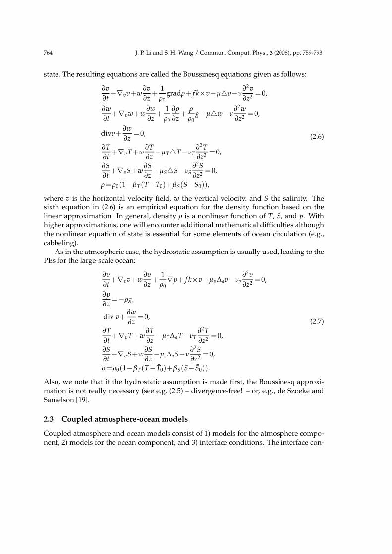
Figure 1: A bifurcated attractor containing 4 nodes (the points a, b, c, and d), 4 saddles (the points e, f, g,h), and orbits connecting these 8 points.

The bifurcation theory has been applied to various problems from science and engi-neering, including, in particular, the Kuramoto-Sivashinshy equation, the Cahn-Hillardequation, the Ginzburg-Landau equation, Reaction-Diffusion equations in Biology andChemistry, and the Benard convection problem and the Taylor problem in classical fluidmechanics; see a recent book by Ma and Wang [100]. For applications to geophysicalfluid dynamics problems, we have carried out the detailed bifurcation and stability anal-ysis for 1) the stratified Boussinesq equations [47], 2) the doubly-diffusive modes (both2D and 3D) [45, 46].

We proceed with a simple example to illustrate the basic motivation and ideas behindthe attractor bifurcation theory. For x=(x1,x2)∈R2, the system

x=λx−(x31,x3

2)+o(|x|3)

bifurcates from (x,λ)=(0,0) to an attractor Σλ =S1. This bifurcated attractor is as shownin Fig. 1, and contains exactly 4 nodes (the points a, b, c, and d), 4 saddles (the pointse, f, g, h), and orbits connecting these 8 points. From the physical transition point ofview, as λ crosses 0, the new state after the system undergoes a transition is representedby the whole bifurcated attractor Σλ, rather than any of the steady states or any of theconnecting orbits. The connecting orbits represents transient states. Note that the globalattractor is the 2D region enclosed by Σλ. We point out here that the bifurcated attractoris different from the study on global attractors of a dissipative dynamical system-bothfinite and infinite dimensional. Global attractor studies the global long time dynamics(see among others [2, 17, 18, 27]), while the bifurcated attractor provides a natural objectfor studying dynamical transitions [100, 103, 105].


One important characteristic of the new attractor bifurcation theory is related to theasymptotic stability of the bifurcated solutions. This characteristic can be viewed as fol-lows. First, as an attractor itself, the bifurcated attractor has a basin of attractor, andconsequently is a useful object to describe local transitions. Second, with detailed clas-sification of the solutions in the bifurcated attractor, we are able to access not only theasymptotic stability of the bifurcated attractor, but also the stability of different solutionsin the bifurcated attractor, providing a more complete understanding of the transitionsof the physical system as the system parameter varies. Third, as Kirchgassner [59] indi-cated, an ideal stability theorem would include all physically meaningful perturbationsand today we are still far from this goal. In addition, fluid flows are normally time de-pendent. Therefore bifurcation analysis for steady state problems provides in generalonly partial answers to the problem, and is not enough for solving the stability problem.Hence from the physical point of view, attractor bifurcation provides a nature tool forstudying transitions for deterministic systems.

6.2 A brief account of the attractor bifurcation theory

We now briefly present this new attractor bifurcation theory and refer the interested read-ers to [100, 105] for details of the theory and its various applications.

We start with a basic state ϕ of the system, a steady state solution of (3.1). Thenconsider ϕ=u+ ϕ. Then (3.1) becomes

du

dt= Lλu+G(u,λ), (6.1)

u(0)=u0, (6.2)

where H and H1 are two Hilbert spaces such that H1→H be a dense and compact inclu-sion.

The mapping u : [0,∞)→ H is the unknown function, λ∈R is the system parameter,and Lλ :H1→H is a family of linear completely continuous fields depending continuouslyon λ∈R, such that

Lλ =−A+Bλ a sectorial operator,

A : H1→H a linear homeomorphism,

Bλ : H1→H a linear compact operator.

(6.3)

It is known that Lλ generates an analytic semigroup e−tLλt≥0 and we can define frac-tional power operators Lα

λ for α ∈ R with domain Hα = D(Lαλ) such that Hα1

⊂ Hα2 iscompact if α1 >α2, H = H0 and H1 = Hα=1.

Furthermore, we assume that for some θ <1 the nonlinear operator G(·,λ) : Hθ →H0

is a Cr bounded operator (r≥1), and

G(u,λ)= o(‖u‖θ), ∀λ∈R. (6.4)


λ

H

λλ0

Σ

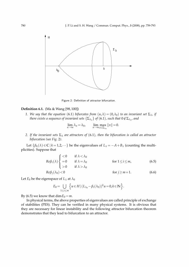
Figure 2: Definition of attractor bifurcation.

Definition 6.1. (Ma & Wang [98, 100])

1. We say that the equation (6.1) bifurcates from (u,λ) = (0,λ0) to an invariant set Σλ, ifthere exists a sequence of invariant sets Σλn

of (6.1), such that 0 /∈Σλn, and

limn→∞

λn =λ0, limn→∞

maxx∈Σλn

‖x‖=0.

2. If the invariant sets Σλ are attractors of (6.1), then the bifurcation is called an attractorbifurcation (see Fig. 2).

Let βk(λ)∈C | k = 1,2,··· be the eigenvalues of Lλ =−A+Bλ (counting the multi-plicities). Suppose that

Reβi(λ)

<0 if λ<λ0

=0 if λ=λ0

>0 if λ>λ0

for 1≤ i≤m, (6.5)

Reβ j(λ0)<0 for j≥m+1. (6.6)

Let E0 be the eigenspace of Lλ at λ0

E0 =⋃

1≤i≤m

u∈H | (Lλ0−βi(λ0))

ku=0,k∈N

.

By (6.5) we know that dimE0 =m.In physical terms, the above properties of eigenvalues are called principle of exchange

of stabilities (PES). They can be verified in many physical systems. It is obvious thatthey are necessary for linear instability and the following attractor bifurcation theoremdemonstrates that they lead to bifurcation to an attractor.


Theorem 6.1 (Ma & Wang [98, 100]). Assume that (6.5) and (6.6) hold true, and let u = 0 bea locally asymptotically stable equilibrium point of (6.1) at λ = λ0. Then we have the followingassertions.

1. Eq. (6.1) bifurcates from (u,λ)=(0,λ0) to an attractor Σλ for λ>λ0 with m−1≤dimΣλ≤m, which is an (m−1)-dimensional homological sphere.

2. For any uλ∈Σλ, uλ can be expressed as uλ =vλ+o(‖vλ‖), where vλ ∈E0.

3. There exists a neighborhood U⊂H of u=0 such that Σλ attracts U\Γ, where Γ is the stablemanifold of u=0 with codimension m. In particular, if u=0 is global asymptotically stablefor (6.1) at λ=λ0 and (6.1) has a global attractor for any λ near λ0, then Σλ attracts H\Γ.

With this general theorem, along with other important ingredients addressed in Maand Wang [100,105], at our disposal, the main strategy to conduct the bifurcation analysisconsists of 1) the existence of attractor bifurcation, and 2) classification of solutions in thebifurcated attractor. We refer the interested readers to the books [100, 105] for details; seealso the discussion below on the Rayleigh-Benard convection.

6.3 Dynamic bifurcation in classical fluid dynamics

The new dynamic bifurcation theory has been naturally applied to problems in fluid dy-namics, including the Rayleigh-Benard convection, the Taylor problem, and the parallelshear flows, by Ma and Wang and their collaborators. The study of these basic problemson the one hand plays an important role in understanding the turbulent behavior of fluidflows, and on the other hand often leads to new insights and methods toward solutionsof other problems in sciences and engineering.

To illustrate the main ideas of the applications of the theory, we consider now theRayleigh-Benard convection problem. Linear theory of the Rayleigh-Benard problemwere essentially derived by physicists; see, among others, Chandrasekhar [10] andDrazin and Reid [23]. Bifurcating solutions of the nonlinear problem were first con-structed formally by Malkus and Veronis [109]. The first rigorous proofs of the existenceof bifurcating solutions were given by Yudovich [156, 157] and Rabinowitz [123]. Yu-dovich proved the existence of bifurcating solutions by a topological degree argument.Earlier, however, Velte [143] had proved the existence of branching solutions of the Tay-lor problem by a topological degree argument as well. The have been many studies sincethe above mentioned early works. However, as we shall see, a rigorous and complete un-derstanding of the problem is not available until the recent work by Ma and Wang usingthe attractor bifurcation theory.

To illustrate the ideas, we start by recalling the basic set-up of the problem. Let theRayleigh number be

R=gα(T0−T1)h3

(κν).


The Benard convection is modeled by the Boussinesq equations. In their nondimensionalform, these equations are written as follows:

1

Pr

[

∂u

∂t+(u·∇)u+∇p

]

−∆u−√

RTk=0,

∂T

∂t+(u·∇)T−

√Ru3−∆T =0,

div u=0.

(6.7)

Here the unknown functions are (u,T,p), which are the deviations from the basic field.The non-dimensional domain is Ω=D×(0,1)⊂R3, where D⊂R2 is an open set. The coor-dinate system is given by x=(x1,x2,x3)∈R3. They are supplemented with the followinginitial value conditions

(u,T)=(u0,T0) at t=0. (6.8)

Boundary conditions are needed at the top and bottom and at the lateral boundary∂D×(0,1). At the top and bottom boundary (x3 = 0,1), either the so-called rigid or freeboundary conditions are given

T =0, u=0 (rigid boundary),

T =0, u3 =0,∂(u1,u2)

∂x3=0 (free boundary).

(6.9)

Different combinations of top and bottom boundary conditions are normally used indifferent physical setting such as rigid-rigid, rigid-free, free-rigid, and free-free.

On the lateral boundary ∂D×[0,1], one of the following boundary conditions are usu-ally used:

1. Periodic condition:

(u,T)(x1+k1L1,x2+k2L2,x3)=(u,T)(x1,x2,x3), (6.10)

for any k1,k2∈Z.

2. Dirichlet boundary condition:

u=0, T =0 (or∂T

∂n=0); (6.11)

3. Free boundary condition:

T =0, un =0,∂uτ

∂n=0, (6.12)

where n and τ are the unit normal and tangent vectors on ∂D×[0,1] respec-tively, and un =u·n, uτ =u·τ.


By using the attractor bifurcation theory, the following results have been obtained byMa and Wang in [97, 100, 104, 105].

(1) When the Rayleigh number R crosses the first critical Rayleigh number Rc, theRayleigh-Benard problem bifurcates from the basic state to an attractor AR, homo-logic to Sm−1, where m is the multiplicity of Rc as an eigenvalue of the linearizedproblem near the basic solution, for all physically sound boundary conditions, re-gardless of the geometry of the domain and the multiplicity of the eigenvalue Rc

for the linear problem

(2) Consider the 3D Benard convection in Ω = (0,L1)×(0,L2)×(0,1) with free top-bottom and periodic horizontal boundary conditions, and with

k21

L21

+k2

2

L22

=1

8for some k1,k2∈Z. (6.13)

Then

AR =

S5 if L2 =√

k2−1L1, k=2,3,··· ,

S3 otherwise.(6.14)

(3) For the 3D Benard convection in Ω = (0,L)2×(0,1) with free boundary conditionsand with

0< L2<

2−21/3

21/3−1. (6.15)

The bifurcated attractor AR consists of exactly eight singular points and eight hete-roclinic orbits connecting the singular points, as shown in Figure 1, with 4 of thembeing minimal attractors, and the other 4 saddle points.

The proof of these results is carried out in the following steps:

1) It is classical to put the Boussinesq equations (6.7) in the abstract form (6.1). Thenit is easy to see that the linearized operator is a self-adjoint operator., and bothconditions (6.3) and (6.4) are satisfied.

2) As the linearized operator is symmetric, it is not hard to verify the PES (6.5) and(6.6) for the Boussinesq equations.

3) To derive a general attractor theorem for the Benard convection regardless of thedomain and the boundary conditions, we need to verify the asymptotic stability ofthe basic solution (u,T) = 0 at the critical Reynolds number. This can be achievedby a general stability theorem, derived by Ma and Wang in [97].

4) The detailed structure of the solutions in the bifurcated attractor can be derivedusing a new approximation formula for the center manifold function; see Ma andWang [100, 104, 105].


We remark here that the high dimensional sphere Sm−1 contains not only the steadystates generated by symmetry groups inherited in the problem, but also many transientstates, which were completely missed by any classical theories. These transient statesare highly relevant in geophysical fluid dynamics and climate dynamics. We believe theclimate low frequency climate variabilities discussed in the previous section are relatedto certain transient states, and further exploration in this direction are certainly importantand necessary.

6.4 Dynamic bifurcation and stability in geophysical fluid dynamics

As mentioned earlier, the theory has been applied to models in geophysical fluid dynam-ics models including the doubly-diffusive models, and rotating Boussinesq equations.We now briefly address these applications in turn.

ROTATING BOUSSINESQ EQUATIONS: Rotating Boussinesq equations are basic modelin atmosphere and ocean dynamical models. In [47], for the case where the Prandtl num-ber is greater than one, a complete stability and bifurcation analysis near the first criticalRayleigh number is carried out. Second, for the case where the Prandtl number is smallerthan one, the onset of the Hopf bifurcation near the first critical Rayleigh number is es-tablished, leading to the existence of nontrivial periodic solutions. The analysis is basedon a newly developed bifurcation and stability theory for nonlinear dynamical systemsas mentioned above.

DOUBLE-DIFFUSIVE OCEAN MODEL: Double-diffusion was first originally discov-ered in the 1857 by Jevons [51], forgotten, and then rediscovered as an “oceanographiccuriosity” a century later; see among others Stommel, Arons and Blanchard [140], Vero-nis [145], and Baines and Gill [3]. In addition to its effects on oceanic circulation, double-diffusion convection has wide applications to such diverse fields as growing crystals, thedynamics of magma chambers and convection in the sun.

The best known doubly-diffusive instabilities are “salt-fingers” as discussed in thepioneering work by Stern [138]. These arise when hot salty water lies over cold freshwater of a higher density and consist of long fingers of rising and sinking water. A blobof hot salty water which finds itself surrounded by cold fresh water rapidly loses its heatwhile retaining its salt due to the very different rates of diffusion of heat and salt. Theblob becomes cold and salty and hence denser than the surrounding fluid. This tends tomake the blob sink further, drawing down more hot salty water from above giving riseto sinking fingers of fluid.

In [45,46], we present a bifurcation and stability analysis on the doubly-diffusive con-vection. The main objective is to study 1) the mechanism of the saddle-node bifurcationand hysteresis for the problem, 2) the formation, stability and transitions of the typicalconvection structures, and 3) the stability of solutions. It is proved in particular that thereare two different types of transitions: continuous and jump, which are determined explic-itly using some physical relevant nondimensional parameters. It is also proved that thejump transition always leads to the existence of a saddle-node bifurcation and hysteresisphenomena.


However, there are many issues still open, including in particular to use the dynami-cal systems tools developed to study some of the issues raised in the previous sections.

6.5 Stability and transitions of geophysical flows in the physical space

Another important area of studies in geophysical fluid dynamics is to study the structureand its stability and transitions of flows in the physical spaces.

A method to study these important problems in geophysical fluid dynamics is a re-cently developed geometric theory for incompressible flows by Ma and Wang [101]. Thistheory consists of research in directions: 1) the study of the structure and its transi-tions/evolutions of divergence-free vector fields, and 2) the study of the structure and itstransitions of velocity fields for 2-D incompressible fluid flows governed by the Navier-Stokes equations or the Euler equations. The study in the first direction is more kinematicin nature, and the results and methods developed can naturally be applied to other prob-lems of mathematical physics involving divergence-free vector fields. In fluid dynamicscontext, the study in the second direction involves specific connections between the solu-tions of the Navier-Stokes or the Euler equations and flow structure in the physical space.In other words, this area of research links the kinematics to the dynamics of fluid flows.This is unquestionably an important and difficult problem.

Progresses have been made in several directions. First, a new rigorous characteri-zation of boundary layer separations for 2-D viscous incompressible flows is developedrecently by Ma and Wang, in collaboration in part with Michael Ghil [101]. The nature offlow’s boundary layer separation from the boundary plays a fundamental role in manyphysical problems, and often determines the nature of the flow in the interior as well.The main objective of this section is to present a rigorous characterization of the bound-ary layer separations of 2D incompressible fluid flows. This is a long standing problemin fluid mechanics going back to the pioneering work of Prandtl [121] in 1904. No knowntheorem, which can be applied to determine the separation, is available until the recentwork by Ghil, Ma and Wang [36,37], and Ma and Wang [93,96], which provides a first rig-orous characterization. Interior separations are studied rigorously by Ma and Wang [99].The results for both the interior and boundary layer separations are used in Ma andWang [102] for the transitions of the Couette-Poiseuille and the Taylor-Couette-Poiseuilleflows.

Another example in this area is the justification of the roll structure (e.g. rolls) in thephysical space in the Rayleigh-Benard convection by Ma and Wang [97,104]. We note thata special structure with rolls separated by a cross channel flow derived in [104] has notbeen rigorously examined in the Benard convection setting although it has been observedin other physical contexts such as the Branstator-Kushnir waves in the atmospheric dy-namics [7, 66].

With this theory in our disposal, the structure/patterns and their stability and tran-sitions in the underlying physical spaces for those problems in fluid dynamics and ingeophysical fluid dynamics can be classified. In particular, this theory has been used to


study the formation, persistence and transitions of flow structures including boundarylayer separation including the Gulf separation, the Hadley circulation, and the Walkercirculation. Further investigation appears to be utterly important and necessary. In addi-tion, it appears that such theoretical and numerical studies will lead to better predicationson weather and climate regimes.

Acknowledgments

The authors would like to thank two anonymous referees for their insightful comments.The work was supported in part by the grants from the Office of Naval Research, fromthe National Science Foundation, and from the National Nature Science Foundation ofChina (40325013, 40675046).

References

[1] A. Babin, A. Mahalov, and B. Nicolaenko, Fast singular oscillating limits and global regu-larity for the 3D primitive equations of geophysics, M2AN Math. Model. Numer. Anal., 34(2000), 201-222.

[2] A. V. Babin and M. I. Vishik, Regular attractors of semigroups and evolution equations, J.Math. Pure. Appl., 62 (1983), 441-491).

[3] P. G. Baines and A. Gill, On thermohaline convection with linear gradients, J. Fluid Mech.,37 (1969), 289-306.

[4] D. S. Battisti and A. C. Hirst, Interannual variability in a tropical atmosphere-ocean model.influence of the basic state, ocean geometry and nonlinearity, J. Atmos. Sci., 46 (1989), 1687-1712.

[5] V. Bjerknes, Das problem von der wettervorhersage, betrachtet vom standpunkt der.mechanik un der physik, Meteorol. Z., 21 (1904), 17.

[6] A. J. Bourgeois and J. T. Beale, Validity of the quasigeostrophic model for large-scale flow inthe atmosphere and ocean, SIAM J. Math. Anal., 25 (1994), 1023-1068.

[7] G. W. Branstator, A striking example of the atmosphere’s leading traveling pattern, J. Atmos.Sci., 44 (1987), 2310-2323.

[8] C. Cao and E. S. Titi, Global well-posedness of the three-dimensional viscous primitive equa-tions of large scale ocean and atmosphere dynamics, Ann. Math., 166 (2007), 245-267.

[9] P. Cessi and G. R. Ierley, Symmetry-breaking multiple equilibria in quasi-geostrophic, wind-driven flows, J. Phys. Oceanogr., 25 (1995), 1196-1202.

[10] S. Chandrasekhar, Hydrodynamic and Hydromagnetic Stability, Dover Publications, 1981.[11] J. Charney, On the scale of atmospheric motion, Geophys. Publ., 17(2) (1948), 1-17.[12] J. Charney and J. DeVore, Multiple flow equilibria in the atmosphere and blocking, J. Atmos.

Sci., 36 (1979), 1205-1216.[13] J. G. Charney, The dynamics of long waves in a baroclinic westerly current, J. Meteorol., 4

(1947), 135-162.[14] B. Chen, J. Li and R. Ding, Nonlinear local lyapunov exponent and atmospheric predictabil-

ity research, Sci. China, 49(10) (2006), 1111-1120.[15] Z.-M. Chen, M. Ghil, E. Simonnet and S. Wang, Hopf bifurcation in quasi-geostrophic chan-

nel flow, SIAM J. Appl. Math., 64 (2003), 343-368.


[16] J. Chou, Long-Term Numerical Weather Prediction, China Meteorological Press, Beijing,1986 (in Chinese).

[17] P. Constantin and C. Foias, Global Lyapunov exponents, Kaplan-Yorke formulas and thedimension of the attractors for 2D Navier-Stokes equations, Commun. Pur. Appl. Math., 38(1985), 1-27.

[18] P. Constantin, C. Foias and R. Temam, Attractors representing turbulent flows, Mem. Am.Math. Soc., 53 (1985), vii+67.

[19] R. A. de Szoeke and R. M. Samelson, The duality between the boussinesq and non-boussinesq hydrostatic equations of motion, J. Phys. Oceanogr., 32 (2002), 2194-2203.

[20] A. Deloncle, R. Berk, F. D’Andrea and M. Ghil, Weather regime prediction using statisticallearning, J. Atmos. Sci., 64(5) (2007), 1619-1635.

[21] H. A. Dijkstra, Nonlinear Physical Oceanography: A Dynamical Systems Approach to theLarge-Scale Ocean Circulation and El Nino, Kluwer Acad. Publishers, Dordrecht/Norwell,Mass., 2000.

[22] R. Ding and J. Li, Nonlinear finite-time lyapunov exponent and predictability, Phys. Lett. A,364 (2007), 396-400.

[23] P. Drazin and W. Reid, Hydrodynamic Stability, Cambridge University Press, 1981.[24] J. P. Eckmann and D. Ruelle, Ergodic theory of chaos and strange attractors, Rev. Mod. Phys.,

57 (1985), 617-656.[25] P. F. Embid and A. J. Majda, Averaging over fast gravity waves for geophysical flows with

arbitrary potential vorticity, Commun. Part. Diff. Eq., 21 (1996), 619-658.[26] Y. Feliks, M. Ghil and E. Simonnet, Low-frequency variability in the midlatitude baroclinic

atmosphere induced by an oceanic thermal front, J. Atmos. Sci., 64 (2007), 97-116.[27] C. Foias and R. Temam, Some analytic and geometric properties of the solutions of the evo-

lution Navier-Stokes equations, J. Math. Pure. Appl., 58 (1979), 339-368.[28] K. Fraedrich, Estimating weather and climate predictability on attractors, J. Atmos. Sci., 44

(1987), 722-728.[29] I. Gallagher, Applications of Schochet’s methods to parabolic equations, J. Math. Pure. Appl.,

77 (1998), 989-1054.[30] M. Ghil, Advances in sequential estimation for atmospheric and oceanic flows, J. Meteorol.

Soc. Jpn., 75 (1997), 289-304.[31] M. Ghil, M. R. Allen, M. D. Dettinger, K. Ide, D. Kondrashov, M. E. Mann, A. W. Robertson,

A. Saunders, Y. Tian, F. Varadi and P. Yiou, Advanced spectral methods for climatic timeseries, Rev. Geophys., 40(1) (2002), 3.1-3.41.

[32] M. Ghil and S. Childress, Topics in Geophysical Fluid Dynamics: Atmospheric Dynamics,Dynamo Theory, and Climate Dynamics, Springer-Verlag, New York, 1987.

[33] M. Ghil, S. Cohn, J. Tavantzis, K. Bube and E. Isaacson, Applications of estimation theoryto numerical weather prediction, in: L. Bengtsson, M. Ghil and E. Klln (Eds.), DynamicMeteorology: Data Assimilation Methods, Springer-Verlag, 1981, pp. 139-224.

[34] M. Ghil, K. Ide, A. F. Bennett, P. Courtier, M. Kimoto and N. Sato (Eds.), Data Assimilationin Meteorology and Oceanography: Theory and Practice, Meteorological Society of Japanand Universal Academy Press, Tokyo, 1997.

[35] M. Ghil, J.-G. Liu, C. Wang and S. Wang, Boundary-layer separation and adverse pressuregradient for 2-D viscous incompressible flow, Physica D, 197 (2004), 149-173.

[36] M. Ghil, T. Ma and S. Wang, Structural bifurcation of 2-D incompressible flows, IndianaUniv. Math. J., 50 (2001), 159-180.

[37] M. Ghil, T. Ma and S. Wang, Structural bifurcation of 2-D incompressible flows with the


Dirichlet boundary conditions and applications to boundary layer separations, SIAM J.Appl. Math., 65 (2005), 1576-1596.

[38] M. Ghil and P. Malanotte-Rizzoli, Data assimilation in meteorology and oceanography, Adv.Geophys., 33 (1991), 141-266.

[39] M. Ghil and A. W. Robertson, ”Waves” vs. ”particles” in the atmosphere’s phase space: Apathway to long-range forecasting?, Proc. Natl. Acad. Sci. USA, 99 (Suppl. 1) (2002), 2493-2500.

[40] M. Ghil, I. Zaliapin and B. Coluzzi, Boolean delay equations: A simple way of looking atcomplex systems, Physica D, (2007).

[41] A. Gill, Some simple solutions for heat induced tropical circulation, Q. J. Roy. Meteor. Soc.,106 (1980), 447-462.

[42] A. E. Gill, Atmosphere-Ocean Dynamics, Academic Press, 1982.[43] G. Haltiner and R. Williams, Numerical Weather Prediction and Dynamic Meteorology, Wi-

ley, New York, 1980.[44] J. R. Holton, An Introduction to Dynamic Meteorology, 4th Ed., Elsevier Academic Press,

2004.[45] C.-H. Hsia, T. Ma and S. Wang, Attractor bifurcation of double-diffusive convection, ZAA,

to appear; see also ArXiv.org Preprint no. nlin.PS/0611024, (2006).[46] C.-H. Hsia, T. Ma and S. Wang, Bifurcation and stability of two-dimensional double-

diffusive convection, submitted; see also ArXiv.org Preprint no. physics/0611111, (2006).[47] C.-H. Hsia, T. Ma and S. Wang, Stratified rotating boussinesq equations in geophysical

fluid dynamics: Dynamic bifurcation and periodic solutions, submitted; see also ArXiv.orgPreprint no. math-ph/0610087, (2006).

[48] C. Hu, R. Temam and M. Ziane, The primitive equations on the large scale ocean under thesmall depth hypothesis, Discrete Cont. Dyn. Syst., 9 (2003), 97-131.

[49] G. Ierley and V. A. Sheremet, Multiple solutions and advection-dominated flows in thewind-driven circulation. I: Slip, J. Marine Res., 53 (1995), 703-737.

[50] D. Iftimie and G. Raugel, Some results on the Navier-Stokes equations in thin 3D domains,J. Differ. Equations, 169 (2001), 281-331.

[51] W. S. Jevons, On the cirrous form of cloud, London, Edinburgh, Dublin Philos. Mag. J. Sci.Ser. 4, 14 (1857), 22-35.

[52] F. F. Jin, Tropical ocean-atmosphere interaction, the pacific cold tongue, and the el nio south-ern oscillation, Science, 274 (1996), 76-78.

[53] F. F. Jin and M. Ghil, Intraseasonal oscillations in the extratropics: Hopf bifurcation andtopographic instabilities, J. Atmos. Sci., 47 (1990), 3007-3022.

[54] N. Ju, The global attractor for the solutions of the 3d viscous primitive equations, DiscreteCont. Dyn. Syst., 17(1) (2007), 159-179.

[55] K. I. Chang, M. Ghil and C.-C. A. Lai, Transition to aperiodic variability in a wind-drivendouble-gyre circulation model, J. Phys. Oceanogr., 31 (2001), 1260-1286.

[56] J. Kao, D. Flicker, K. Ide and M. Ghil, Estimating model parameters for an impact-producedshock-wave simulation: Optimal use of partial data with the extended kalman filter, J. Com-put. Phys., 214 (2006), 725-737.

[57] E. Kazantsev, Local lyapunov exponents of the quasigeostrophic ocean dynamics, Appl.Math. Comput., 104 (1999), 217-257.

[58] C. L. Keppenne, S. L. Marcus, M. Kimoto and M. Ghil, Intraseasonal variability in a two-layer model and observations, J. Atmos. Sci., 57 (2000), 1010-1028.

[59] K. Kirchgassner, Bifurcation in nonlinear hydrodynamic stability, SIAM Rev., 17 (1975), 652-


683.[60] D. Kondrashov, S. Kravtsov and M. Ghil, Empirical mode reduction in a model of extratrop-

ical low-frequency variability, J. Atmos. Sci., 63(7) (2006), 1859-1877.[61] D. Kondrashov, S. Kravtsov, A. W. Robertson and M. Ghil, A hierarchy of data-based enso

models, J. Climate, 18 (2005), 4425-4444.[62] D. Kondrashov, J. Shen, R. Berk, F. D’Andrea and M. Ghil, Predicting weather regime tran-

sitions in northern hemisphere datasets, Clim. Dynam., 29 (2007), 535-551.[63] D. Kondrashov, Y. Shprits, M. Ghil and R. Thorne, Estimation of relativistic electron lifetimes

in the outer radiation belt: A kalman filtering approach, J. Geophys. Res.-Space Phys., (2007),in press.

[64] S. Kravtsov, D. Kondrashov and M. Ghil, Multilevel regression modeling of nonlinear pro-cesses: Derivation and applications to climatic variability, J. Climate, 18 (2005), 4404-4424.

[65] I. Kukavica and M. Ziane, Existence of strong solutions of the primitive equations of theocean with dirichlet boundary conditions, Nonlinearity, (2007).

[66] K. Kushnir, Retrograding wintertime low-frequency disturbances over the north pacificocean, J. Atmos. Sci., 44 (1987), 2727-2742.

[67] J. F. Lacarra and O. Talagrand, Short-range evolution of small perturbations in a barotropicmodel, Tellus, 40A (1988), 81-95.

[68] R. Laprise, The euler equation of motion with hydrostatic pressure as an independent vari-able, Mon. Weather Rev., 120 (1992), 197-207.

[69] K. M. Lau, P. J. Sheu and I. S. Kang, Multiscale low-frequency circulation modes in the globalatmosphere, J. Atmos. Sci., 51 (1994), 1169-1193.

[70] B. Legras and M. Ghil, Persistent anomalies, blocking and variations in atmospheric pre-dictability, J. Atmos. Sci., 42 (1985), 433-471.

[71] J. Li and J. Chou, The property of solutions for the equations of large-scale atmosphere withthe non-stationary external forcings, Chinese Sci. Bull., 41 (1996), 587-590.

[72] J. Li and J. Chou, Source of atmospheric multiple equilibria, Chinese Sci. Bull., 41 (1996),2074-2077.

[73] J. Li and J. Chou, The effects of external forcing, dissipation and nonlinearity on the solutionsof atmospheric equations, Acta Meteor. Sinica, 11 (1997), 57-65.

[74] J. Li and J. Chou, Existence of atmosphere attractor, Sci. China Ser. D, 40 (1997), 215-224.[75] J. Li and J. Chou, Further study on the properties of operators of atmospheric equations and

the existence of attractor, Acta Meteor. Sinica, 11 (1997), 216-223.[76] J. Li and J. Chou, Asymptotic properties of the moist atmospheric dynamical equations, Acta

Meteor. Sinica, 12 (1998), 187-198.[77] J. Li and J. Chou, The qualitative theory on the dynamical equations of atmospheric motion

and its applications, Chinese J. Atmos. Sci., 22 (1998), 348-360.[78] J. Li and J. Chou, Asymptotic behavior of the solutions of atmospheric equations with the

topographic effect, Prog. Nat. Sci., 9 (1999), 781-791.[79] J. Li, R. Ding and B. Chen, Review and prospect on the predictability study of the atmo-

sphere, in: Frontier and Prospect of Atmospheric Sciences at the Beginning of the 21th Cen-tury, China Meteorology Press, Beijing, 2006, pp. 96-104.

[80] J. Li, Q. Zeng and J. Chou, Computational uncertainty principle in nonlinear ordinary dif-ferential equations I. Numerical results, Sci. China Ser. E, 43 (2000), 449-460.

[81] J. Li, Q. Zeng and J. Chou, Computational uncertainty principle in nonlinear ordinary dif-ferential equations II. Theoretical analysis, Sci. China Ser. E, 44 (2001), 55-74.

[82] J. L. Lions, O. P. Manley, R. Temam and S. Wang, Physical interpretation of the attractor


dimension for the primitive equations of atmospheric circulation, J. Atmos. Sci., 54 (1997),1137-1143.

[83] J. L. Lions, R. Temam and S. Wang, New formulations of the primitive equations of theatmosphere and applications, Nonlinearity, 5 (1992), 237-288.

[84] J. L. Lions, R. Temam and S. Wang, On the equations of large-scale ocean, Nonlinearity, 5(1992), 1007-1053.

[85] J. L. Lions, R. Temam and S. Wang, Models of the coupled atmosphere and ocean (CAO I),Comput. Mech. Adv., 1 (1993), 3-54.

[86] J. L. Lions, R. Temam and S. Wang, Geostrophic asymptotics of the primitive equations ofthe atmosphere, Topol. Meth. Nonlinear Anal., 4 (1994), 253-287.

[87] J. L. Lions, R. Temam and S. Wang, Mathematical study of the coupled models of atmosphereand ocean (CAO III), J. Math. Pure. Appl., 73(2) (1995), 105-163.

[88] J. L. Lions, R. Temam and S. Wang, Splitting-up methods and numerical analysis of somemultiscale problems, Comput. Fluid Dyn. J., 5(2) (1996), 157-202.

[89] J. L. Lions, R. Temam and S. Wang, A simple global model for the general circulation of theatmosphere, Commun. Pur. Appl. Math., 50 (1997), 707-752.

[90] E. N. Lorenz, Deterministic nonperiodic flow, J. Atmos. Sci., 20 (1963), 130-141.[91] E. N. Lorenz, The mechanics of vacillation, J. Atmos. Sci., 20 (1963), 448-464.[92] E. N. Lorenz, Atmospheric predictability as revealed by naturally ocurring analogues, J.

Atmos. Sci., 26 (1969), 636-646.[93] T. Ma and S. Wang, Structure of 2D incompressible flows with the Dirichlet boundary con-

ditions, Discrete Cont. Dyn. Syst. Ser. B, 1 (2001), 29-41.[94] T. Ma and S. Wang, Topology of 2-d incompressible flows and applications to geophysical

fluid dynamics, Rev. R. Acad. Cien. Serie A. Mat. (RACSAM), 96 (2002), 447-459.[95] T. Ma and S. Wang, Rigorous characterization of boundary layer separations, in: Computa-

tional Fluid and Solid Mechanics 2003, Elsevier, 2003.[96] T. Ma and S. Wang, Boundary layer separation and structural bifurcation for 2-D incom-

pressible fluid flows, Discrete Cont. Dyn. Syst. Ser. A, 10(1-2) (2004), 459-472.[97] T. Ma and S. Wang, Dynamic bifurcation and stability in the Rayleigh-Benard convection,

Commun. Math. Sci., 2(2) (2004), 159-183.[98] T. Ma and S. Wang, Dynamic bifurcation of nonlinear evolution equations and applications,

Chinese Ann. Math. B, 26 (2005), 185-206.[99] T. Ma and S. Wang, Interior structural bifurcation and separation of 2D incompressible flows,

J. Math. Phys., 45 (2004), 1762-1776.[100] T. Ma and S. Wang, Bifurcation Theory and Applications, World Scientific, 2005.[101] T. Ma and S. Wang, Geometric Theory of Incompressible Flows with Applications to Fluid

Dynamics, vol. 119 of Mathematical Surveys and Monographs, American Mathematical So-ciety, Providence, RI, 2005.

[102] T. Ma and S. Wang, Boundary-layer and interior separations in the taylor-couette-poiseuilleflow, arXiv:math-ph/0701073, (2007).

[103] T. Ma and S. Wang, Phase Transition Dynamics in Nonlinear Sciences, 2007, in preparation.[104] T. Ma and S. Wang, Rayleigh-benard convection: Dynamics and structure in the physical

space, Commun. Math. Sci., 5(3) (2007), 553-574.[105] T. Ma and S. Wang, Stability and Bifurcation of Nonlinear Evolution Equations, Chinese

Academic Press, 2007.[106] R. A. Madden and P. R. Julian, Detection of a 40-50 day oscillation in the zonal wind in the

tropical pacific, J. Atmos. Sci., 28 (1971), 702-708.


[107] R. A. Madden and P. R. Julian, Description of global-scale circulation cells in the tropicswith a 40-50 day period, J. Atmos. Sci., 29 (1972), 1109-1123.

[108] A. J. Majda and X. Wang, Non-linear Dynamics and Statistical Theories for Basic Geophys-ical Flows, Cambridge University Press, Cambridge, 2006.

[109] W. V. R. Malkus and G. Veronis, Finite amplitude cellular convection, J. Fluid Mech., 4(1958), 225-260.

[110] S. Meacham and P. Berloff, Instability of a steady, barotropic, wind driven circulation, J.Mar. Res., 55 (1997), 885-913.

[111] S. Meacham and P. Berloff, On the stability of the wind-driven circulation, J. Mar. Res., 56(1998), 937-993.

[112] S. P. Meacham, Low-frequency variability in the wind-driven circulation, J. Phys.Oceanogr., 30 (2000), 269-293.

[113] J. Meinckel, D. Quadfasel, W. Berger, K. Brander, R. Dickson, P. Haugan, M. Latif,J. Marotzke, J. Marshall, J. Minster, J. Ptzold, G. Parilla, W. de Ruijter and F. Schott, Vari-ability of the thermohaline circulation (thc), in: G. Wefer, F. Lamy and F. Mantoura (Eds.),Marine Science Frontiers for Europe, Springer-Verlag, 2003, pp. 39-60.

[114] M. Mu, Nonlinear singular vectors and nonlinear singular values, Sci. China Ser. D, 43(2000), 375-385.

[115] B. Nadiga and B. Luce, Global bifurcation of shilnikov type in a double gyre ocean model,J. Phys. Oceanogr., 31 (2001), 2669-2690.

[116] J. D. Neelin, D. S. Battisti, A. C. Hirst, F.-F. Jin, Y. Wakata, T. Yamagata and S. E. Zebiak,Enso theory, J. Geophys. Res., 103 (1998), 14261-14290.

[117] J. Pedlosky, Resonant topographic waves in barotropic and baroclinic flows, J. Atmos. Sci.,38 (1981), 2626-2641.

[118] J. Pedlosky, Geophysical Fluid Dynamics, 2nd ed., Springer-Verlag, New York, 1987.[119] J. P. Peixoto and A. H. Oort, Physics of Climate, American Institute of Physics, New York,

1992.[120] N. A. Phillips, The general circulation of the atmosphere: A numerical experiment, Q. J.

Roy. Meteor. Soc., 82 (1956), 123-164.[121] L. Prandtl, in: Verhandlungen des dritten internationalen Mathematiker-Kongresses, Hei-

delberg, 1904, Leipeizig, 1905, pp. 484-491.[122] C. Qiu and J. Chou, Four-dimensional data assimilation method based on svd: Theoretical

aspect, Theor. Appl. Climatol., 83 (2006), 51-57.[123] P. H. Rabinowitz, Existence and nonuniqueness of rectangular solutions of the Benard prob-

lem, Arch. Rational Mech. Anal., 29 (1968), 32-57.[124] S. Rahmstorf, Thermohaline ocean circulation, in: S. A. Elias (Ed.), Encyclopedia of Quater-

nary Sciences, Elsevier, Amsterdam, 2006.[125] C.-G. Rossby, On the solution of problems of atmospheric motion by means of model ex-

periment, Mon. Wea. Rev., 54 (1926), 237-240.[126] C.-G. Rossby, On the mutual adjustment of pressure and velocity distributions in certain

simple current systems, II., J. Mar. Res., 5 (1938), 239-263.[127] F. F. J. S. Jiang and M. Ghil, Multiple equilibria, periodic, and aperiodic solutions in a wind-

driven, double-gyre, shallow-water model, J. Phys. Oceanogr., 25 (1995), 764-786.[128] M. L. Salby, Fundamentals of Atmospheric Physics, Academic Press, 1996.[129] R. Samelson, R. Temam, C. Wang and S. Wang, Surface pressure Poisson equation formu-

lation of the primitive equations: Numerical schemes, SIAM J. Numer. Anal., 41 (2003),1163-1194.


[130] R. Samelson, R. Temam and S. Wang, Some mathematical properties of the planetarygeostrophic equations for large-scale ocean circulation, Appl. Anal., 70 (1998), 147-173.

[131] R. Samelson, R. Temam and S. Wang, Remarks on the planetary geostrophic model of gyrescale ocean circulation, Differ. Integral Equat., 13 (2000), 1-14.

[132] P. S. Schopf and M. J. Suarez, Vacillations in a coupled ocean-atmosphere model, J. Atmos.Sci., 45 (1987), 549-566.

[133] J. Shen and S. Wang, A fast and accurate numerical scheme for the primitive equations ofthe atmosphere, SIAM J. Numer. Anal., 36 (1999), 719-737.

[134] E. Simonnet, M. Ghil, K. Ide, R. Temam and S. Wang, Low-frequency variability in shallow-water models of the wind-driven ocean circulation. Part I: Steady-state solutions, J. Phys.Oceanogr., 33 (2003), 712-728.

[135] E. Simonnet, M. Ghil, K. Ide, R. Temam and S. Wang, Low-frequency variability in shallow-water models of the wind-driven ocean circulation. Part II: Time-dependent solutions, J.Phys. Oceanogr., 33 (2003), 729-752.

[136] J. M. Slingo, P. Inness, R. Neale, S. Woolnough and G.-Y. Yang, Scale interactions on diurnalto seasonal timescales and their relevance to model systematic errors, Ann. Geophys., 46(2003), 139-155.

[137] S. Speich, H. Dijkstra and M. Ghil, Successive bifurcations in a shallow-water model, ap-plied to the wind-driven ocean circulation, Nonlinear Proc. Geophys., 2 (1995), 241-268.

[138] M. E. Stern, The “salt fountain” and thermohaline convection, Tellus, 12 (1960), 172-175.[139] H. Stommel, Thermohaline convection with two stable regimes of flow, Tellus, 13 (1961),

224-230.[140] H. Stommel, A. Arons and D. Blanchard, An oceanographical curiosity: the perpetual salt

fountain, Deep-Sea Res., 3 (1956), 152-153.[141] R. Temam and M. Ziane, Some mathematical problems in geophysical fluid dynamics, in:

Handbook of Mathematical Fluid Dynamics, Vol. III, North-Holland, Amsterdam, 2004,pp. 535-657.

[142] R. B. Thorpe, J. M. Gregory, T. C. Johns, R. A. Wood and J. F. B. Mitchell, Mechanismsdetermining the atlantic thermohaline circulation response to greenhouse gas forcing in anon-flux-adjusted coupled climate model, J. Climate, 14 (2001), 3102-3116.

[143] W. Velte, Stabilitat and verzweigung stationarer losungen der davier-stokeschen gleichun-gen, Arch. Rat. Mech. Anal., 22 (1966), 1-14.

[144] G. Veronis, An analysis of wind-driven ocean circulation with a limited fourier components,J. Atmos. Sci., 20 (1963), 577-593.

[145] G. Veronis, On finite amplitude instability in the thermohaline convection, J. Mar. Res., 23(1965), 1-17.

[146] G. Veronis, Wind-driven ocean circulation, part II: Numerical solution of the nonlinearproblem, Deep-Sea Res., 13 (1966), 31-55.

[147] J. von Neumann, Some remarks on the problem of forecasting climatic fluctuations, in: R. L.Pfeffer (Ed.), Dynamics of Climate, Pergamon Press, 1960, pp. 9-12.

[148] B. Wang, Theory, in: Intraseasonal Variability in the Atmosphere-Ocean Climate System,Praxis, Chichester, U.K., 2005, pp. 307-360.

[149] J. Wang, J. Li and J. Chou, Comparison and error analysis of two 4-dimensional SVD dataassimilation schemes, Chinese J. Atmos. Sci., 31 (2007), in press.

[150] S. Wang, On solvability for the equations of the large-scale atmospheric motion, Ph.D. The-sis, Lanzhou University, China, 1988.

[151] S. Wang, J. P. Huang and J. F. Chou, Some properties of the solutions of the large-scale equa-


tions of atmosphere–nonlinear adjustment process by exterior steady sources, Sci. China Ser.B, 33 (1990), 476-484.

[152] W. M. Washington and C. L. Parkinson, An Introduction to Three-Dimensional ClimateModeling, Oxford University Press, Oxford, 1986.

[153] A. Wolf, J. B. Swift, H. Swinney and J. Vastano, Determining lyapunov exponents from atime series, Physica D, 16 (1985), 285-317.

[154] Y. Wu, M. Mu, Q. Zeng and Y. Li, Weak solutions to a model of climate dynamics, NonlinearAnal. Real World Appl., 2 (2001), 507-521.

[155] S. Yoden and M. Nomura, Finite-time Lyapunov stability analysis and its application toatmospheric predictability, J . Atmos. Sci., 50 (1993), 1531-1543.

[156] V. I. Yudovich, Free convection and bifurcation, J. Appl. Math. Mech., 31 (1967), 103-114.[157] V. I. Yudovich, Stability of convection flows, J. Appl. Math. Mech., 31 (1967), 272-281.[158] S. E. Zebiak and M. A. Cane, A model el niosouthern oscillation, Mon. Wea. Rev., 115 (1987),

2262-2278.[159] Q. C. Zeng, Mathematical and Physical Foundations of Numerical Weather Prediction, Sci-

ences Press, Beijing, 1979.[160] C. Zhang, Madden-Julian oscillation, Rev. Geophys., 43 (2003).[161] C. Ziehmann, L. A. Smith and J. Kurths, Localized Lyapunov exponents and the prediction

of predictability, Phys. Lett. A, 271 (2000), 237-251.

Date post:	10-Jul-2018
Category:	Documents
Upload:	vuonghanh
View:	219 times
Download:	0 times

Some Mathematical and Numerical Issues in ...fluid/paper/73.pdf · Some Mathematical and Numerical...

Documents