Some models of beta-generated distributions with ... · Beta-generated distributions Some models of...

Beta-generated distributions

Some models of beta-generated

distributions with applications in finance

Sarabia Alegrıa, Jose Marıa ([email protected])

Prieto Mendoza, Faustino ([email protected])

Jorda Gil, Vanesa ([email protected])

Remuzgo Perez, Lorena ([email protected])

Departamento de Economıa, Universidad de Cantabria

Avda. de los Castros s/n, 39005 Santander, Espana

RESUMEN

Las caracterısticas empıricas de las series de datos financieros han motivado el estudio

de clases de distribuciones flexibles que incorporan propiedades tales como la asimetrıa y

el peso de las colas. En este trabajo se propone el uso de algunos modelos de distribuciones

generadas por la beta y distribuciones generalizadas generadas por la beta (ver Eugene

et al., 2002 y Jones, 2004), para la modelizacion de datos financieros. En particular, se

estudian dos clases de distribuciones t asimetricas, propuestas por Jones y Faddy (2003)

y Alexander et al. (2012). La primera familia depende de dos parametros de forma que

controlan la asimetrıa y el peso de las colas, y la segunda familia incluye un parametro

adicional. Obtenemos expresiones analıticas para la funcion de distribucion, la funcion

de cuantiles y los momentos, ası como para algunas cantidades utiles en econometrıa

financiera, incluyendo el valor en riesgo. Se obtienen varias representaciones estocasticas

de estas familias en terminos de distribuciones estadısticas de uso habitual. Proponemos

algunas extensiones multivariantes y estudiamos algunas de sus propiedades. Por ultimo,

incluimos una aplicacion empırica con datos reales.

XXIV Jornadas de ASEPUMA y XII Encuentro InternacionalAnales de ASEPUMA n 24:A401

1

Sarabia, JM; Prieto, F.; Jorda, V.; Remuzgo, L.

Palabras clave: Distribuciones asimetricas; valor en riesgo; extensiones multivariantes.

Area tematica: Aspectos Cuantitativos de Problemas Economicos y Empresariales con

incertidumbre.


2


ABSTRACT

Empirical features of many financial data series have motivated the study of

flexible classes of distributions which can incorporate properties such as skewness

and fat-tailedness. In this paper we propose the use of some models of beta-generated

and generalized beta-generated distributions (see Eugene et al., 2002 and Jones,

2004), for modelling financial data. In particular, we study two classes of skew t

distributions, proposed by Jones and Faddy (2003) and Alexander et al. (2012).

The first family depends on two shape parameters which control the skewness and

the tail weight, and the second family includes an extra parameter. We obtain

analytical expressions for the cumulative distribution function, quantile function and

moments, and some quantities useful in financial econometrics, including the value

at risk. We provide several stochastic representations for these families in terms of

usual distributions functions. We also propose some multivariate extensions and we

explore some of their properties. Finally, and empirical application with real data

is provided.


3


1 INTRODUCTION

Empirical features of many financial data series have motivated the study of

flexible classes of distributions which can incorporate properties such as skewness

and fat-tailedness.

The student t distribution is used in financial econometrics and risk manage-

ment to model the conditional asset returns (see Bollerslev, 1987). However, this

model does not fully describe the empirical regularities of many financial data. In

this sense, there are several proposals of skewed Student’s t distributions to model

skewness and fat-tail in conditional distributions of financial returns. Some previous

model have been proposed by Theodossiou (1998), Jones and Faddy (2003), Azzalini

and Capitanio (2003) and Zhu and Galbraith (2010) among others.

In this paper we propose the use of some models of beta-generated and gen-

eralized beta-generated distributions (see Eugene et al., 2002 and Jones, 2004), for

modelling financial data. These families of distributions have been used extensively

in the recent statistical literature about distribution theory. In this research, we

study two classes of skew t distributions, proposed by Jones and Faddy (2003) and

Alexander et al. (2012). The first family depends on two shape parameters which

control the skewness and the tail weight, and the second family includes an extra pa-

rameter. We obtain analytical expressions for the cumulative distribution function,

quantile function and moments, and some quantities useful in financial economet-

rics, including the value at risk. We provide several stochastic representations for

these families in terms of usual distributions functions. We also propose some mul-

tivariate extensions and we explore some of their properties. Finally, and empirical

application with real data is provided.

The contents of this paper are as follows. In Section 2 we present some basic

properties of the class of the BG distributions. In Section 3 we presents two classes of

skew-t distributions. Section 4 we consider some financial risk measures. In Section


4


5 we introduce some multivariate versions of the two classes of skew t distributions,

and some of their properties are studied. Some applications with real data are

included in Section 6. Finally, some conclusions are given in Section 7.

2 THE CLASS OF BETA-GENERATED AND

GENERALIZED BETA-GENERATED DISTRI-

BUTIONS

In this section we present basic properties of the class of BG distributions. We

begin with an initial baseline probability density function (PDF) f(x), where the

corresponding cumulative distribution function (CDF) is represented by F (x). The

class of BG distributions is defined in terms of the PDF by (a, b > 0),

gF (x; a, b) = [B(a, b)]−1f(x)F (x)a−1[1− F (x)]b−1, (1)

where B(a, b) = Γ(a)Γ(b)/Γ(a + b) denotes the classical beta function. A random

variable X with PDF (1) will be denoted by X ∼ BG(a, b;F ). If a = i and b =

n− i+ 1 in (1), we obtain the PDF of the i-th order statistic from F (Jones, 2004).

Below, we highlight some representative values of a and b,

• If a = b = 1, gF = f .

• If a = n and b = 1, we obtain the distribution of the maximum.

• If a = 1 and b = n, we obtain the distribution of the minimum.

• If a 6= b, we obtain a family of skew distributions.

Parameters a and b control the tailweight of the distribution. Specifically, the a

parameter controls left-hand tailweight and the b parameter controls the right-hand


5


tailweight of the distribution. On the other hand, if a = b yields a symmetric

sub-family, with a controlling tailweight. In this sense, the BG distribution accom-

modates several kind of tails. For example (see Jones, 2004),

• Potential tails: If f ∼ x−(α+1) and α > 0, when x→∞ gF ∼ x−bα−1,

• Exponential tails: If f ∼ e−αx and β > 0, then gF ∼ e−bβx if x→∞

The CDF associated to (1) is,

GF (x; a, b) = IF (x)(a, b),

where IF (x)(·, ·) denotes the incomplete beta ratio.

If B ∼ Be(a, b) represents the classical beta distribution, a simple stochastic

representation of (1) is,

X = F−1(B). (2)

This representation (2) permits a direct simulation of the values of a random variable

with PDF (1), which can be also used for generating multivariate versions of the

BG distribution. The raw moments of a BG distribution can be obtained by,

E[Xr] = E[{F−1(B)}r], r > 0.

An important number of new classes of distributions have been proposed using this

methodology.

Some extensions of this family have been proposed by Alexander and Sarabia

(2010), Alexander et al. (2012) and Cordeiro and de Castro (2011).

The PDF of the generalized beta-generated is given by,

gF (x; a, b, c) = c[B(a, b)]−1f(x)F (x)ac−1[1− F (x)c]b−1. (3)


6


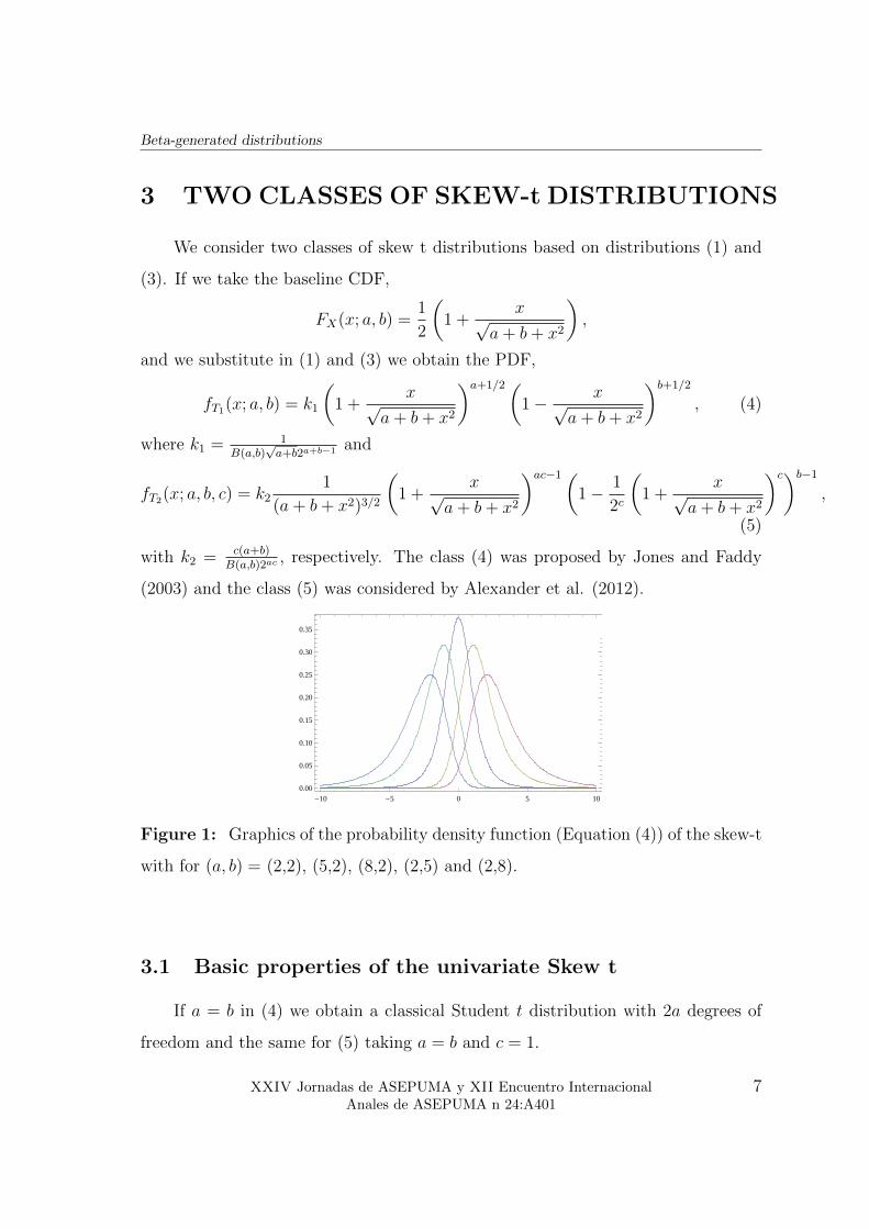
3 TWO CLASSES OF SKEW-t DISTRIBUTIONS

We consider two classes of skew t distributions based on distributions (1) and

(3). If we take the baseline CDF,

FX(x; a, b) =1

2

(1 +

x√a+ b+ x2

),

and we substitute in (1) and (3) we obtain the PDF,

fT1(x; a, b) = k1

(1 +

x√a+ b+ x2

)a+1/2(1− x√

a+ b+ x2

)b+1/2

, (4)

where k1 = 1B(a,b)

√a+b2a+b−1 and

fT2(x; a, b, c) = k21

(a+ b+ x2)3/2

(1 +

x√a+ b+ x2

)ac−1(1− 1

2c

(1 +

x√a+ b+ x2

)c)b−1

,

(5)

with k2 = c(a+b)B(a,b)2ac

, respectively. The class (4) was proposed by Jones and Faddy

(2003) and the class (5) was considered by Alexander et al. (2012).

-10 -5 0 5 100.00

0.05

0.10

0.15

0.20

0.25

0.30

0.35

Figure 1: Graphics of the probability density function (Equation (4)) of the skew-t

with for (a, b) = (2,2), (5,2), (8,2), (2,5) and (2,8).

3.1 Basic properties of the univariate Skew t

If a = b in (4) we obtain a classical Student t distribution with 2a degrees of

freedom and the same for (5) taking a = b and c = 1.


7


-20 -15 -10 -5 0 5 10

0.00

0.05

0.10

0.15

0.20

0.25

0.30

-10 -5 0 5 10 15 20

0.0

0.1

0.2

0.3

0.4

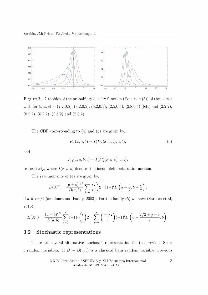
Figure 2: Graphics of the probability density function (Equation (5)) of the skew-t

with for (a, b, c) = (2,2,0.5), (8,2,0.5), (5,2,0.5), (2,5,0.5), (2,8,0.5) (left) and (2,2,2),

(8,2,2), (5,2,2), (2,5,2) and (2,8,2).

The CDF corresponding to (4) and (5) are given by,

Ft1(x; a, b) = I(FX(x; a, b); a, b), (6)

and

Ft2(x; a, b, c) = I(F cX(x; a, b); a, b),

respectively, where I(x; a, b) denotes the incomplete beta ratio function.

The raw moments of (4) are given by,

E(Xr) =(a+ b)r/2

B(a, b)

r∑i=0

(r

i

)2−i(1−)iB

(a− r

2, b− r

2

),

if a, b > r/2 (see Jones and Faddy, 2003). For the family (5) we have (Sarabia et al,

2016),

E(Xr) =(a+ b)r/2

B(a, b)

r∑j=0

(−1)j(r

j

)2−j

∞∑i=0

(−r/2i

)(−1)iB

(a− r/2 + j − i

c, b

).

3.2 Stochastic representations

There are several alternative stochastic representation for the previous Skew

t random variables. If B ∼ B(a, b) is a classical beta random variable, previous


8


random variables can be represented as,

T1(a, b) =

√a+ b(2B − 1)

2√B(1−B)

,

and

T2(a, b, c) =

√a+ b(2B1/c − 1)

2√B1/c(1−B1/c)

,

respectively.

The second kind of stochastic representation is in terms of chi-squared random

variables. If Uν represents a chi-squared random variable with 2ν degrees of freedom,

we have the alternative representations,

T1(a, b) =

√a+ b(Ua − Ub)

2√UaUb

, (7)

and

T2(a, b, c) =

√a+ b

2

2U1/ca − (Ua + Ub)

1/c√U

1/ca ((Ua + Ub)1/c − U1/c

a )

. (8)

4 FINANCIAL RISK MEASURES

In this section we provide closed expressions for the value at risk, for the two

classes of skew t distributions. The value at risk measures of the skew t (4) and (5)

are given by (see Sarabia et al., 2016),

VaRT1 [p; a, b] =

√a+ b(2VaRB[p; a, b]− 1)

2√

VaRB[p; a, b](1− VaRB[p; a, b]), (9)

and

VaRT2 [p; a, b, c] =

√a+ b(2VaR

1/cB [p; a, b]− 1)

2

√VaR

1/cB [p; a, b](1− VaR

1/cB [p; a, b])

, (10)

respectively, with 0 ≤ p ≤ 1, where VaRB[p; a, b] denotes the value at risk of a

classical Be(a, b) distribution. The tail value and risk can be obtained numerically

using Formulas (9) and (10).


9


5 MULTIVARIATE EXTENSIONS

In this section we provide some multivariate versions of the Skew t distributions.

The first multivariate version is a natural extension of the formulas (7) and (8).

Let Ui ∼ χ22νi

and U0 ∼ χ22ν0

, i = 1, 2, . . . ,m be m + 1 independent chi-square

distributions, with 2νi, i = 1, 2, . . . ,m and 2ν0 degrees of freedom respectively, with

νi, ν0 > 0, i = 1, 2, . . . ,m.

The multivariate Skew-t distribution corresponding to first version is defined

by the stochastic representation,

(X

(1)1 , . . . , X(1)

m

)>=

(√ν1 + ν0(U1 − U0)

2√U1U0

, . . . ,

√νm + ν0(Um − U0)

2√UmU0

)>. (11)

The multivariate Skew-t distribution corresponding to the second version is

defined by the stochastic representation,

(X

(2)1 , . . . , X(2)

m

)>=

√νi + ν0

2

2U1/cνi − (Uνi + Uν0)

1/c√U

1/cνi ((Uνi + Uν0)

1/c − U1/cνi )

; i = 1, 2, . . . ,m

(12)

By construction, the marginal distributions belong to the same family. In the

case of (11), the marginal distributions are Skew-t of the first type with parameters

(νi, ν0), i = 1, 2, . . . ,m. For the second multivariate version (12), the marginal distri-

butions are Skew-t of the second type with parameters (νi, ν0, c), for i = 1, 2, . . . ,m.

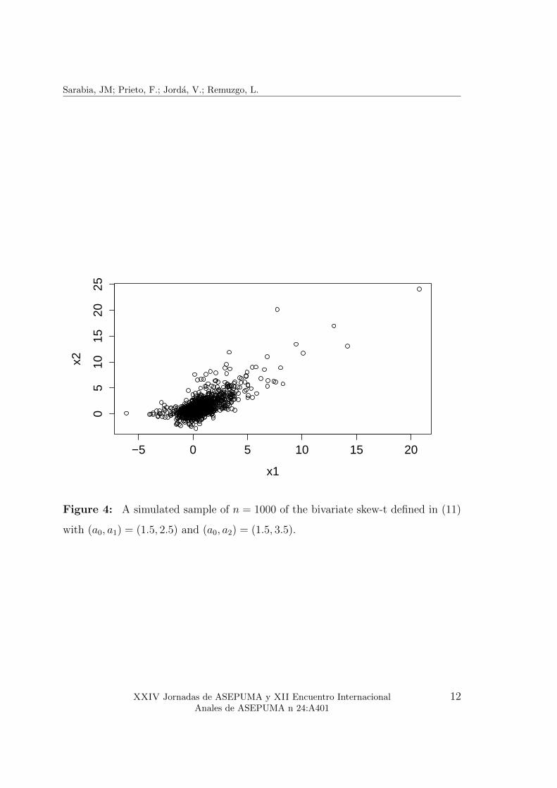
Figures 3 and 4 show two simulated sample of size 1000 from (11) with linear

correlation coefficients 0.485 and 0.756 respectively.

In relation with the dependence structure in (11), we have the following result

(see Sarabia el al. 2016).

Theorem 1 Let consider the multivariate random variable(X

(1)1 , . . . , X

(1)m

)>de-


10


−4 −2 0 2

−2

02

4

x1

x2

Figure 3: A simulated sample of n = 1000 of the bivariate skew-t defined in (11)

with (a0, a1) = (5.5, 4.5) and (a0, a2) = (5.5, 6.5).

fined in (11). Then, the random variables X(1)1 , . . . , X

(1)m are associated. In conse-

quence, the covariance between pairs of variables is always positive.

If we want more flexibility for the marginal distributions, we can use the results

by Sarabia et al (2014) for multivariate beta-generated distributions. For the first

skew-t family, we consider the multivariate distribution,

(X

(1)1 , . . . , X(1)

m

)>=

(F−1i

{Gai

Gai +∑i

j=1Gbj

}, i = 1, 2, . . . ,m

)>,

where Ga represent a classical gamma distribution with shape parameter a. The

marginal distributions are Skew t of the first type with parameters (ai, b1 + · · ·+ bi),

i = 1, 2, . . . ,m.


11


−5 0 5 10 15 20

05

1015

2025

x1

x2

Figure 4: A simulated sample of n = 1000 of the bivariate skew-t defined in (11)

with (a0, a1) = (1.5, 2.5) and (a0, a2) = (1.5, 3.5).


12


6 EMPIRICAL APPLICATION IN FINANCE

In this section we include an application with financial data. We have considered

daily stock-returns data, from 1st January 2015 to 31st December 2015 for five

companies of the Spanish value-weighted index IBEX 35: Amadeus (IT solutions

to tourism industry); BBVA (global financial services); Mapfre (insurance market);

Repsol (energy sector); and Telefonica (information and communications technology

services).

Some relevant information about the data sets used are included in Table 1. For

each company, we have included the sample size n, the maximum and the minimum

daily stock-return in the period considered, the sample mean and standard deviation

and the corresponding skewness and kurtosis. In particular, it can be shown that the

empirical distribution is negatively skewed in four of the five companies considered

and positively skewed in the remaining one.

Table 1

Some relevant information about the datasets considered.

Stock Amadeus BBVA Mapfre Repsol Telefonica

Sample size (n) 261 261 261 261 261

Maximum daily return 0.046286 0.040975 0.050847 0.073466 0.062264

Minimum daily return -0.097367 -0.060703 -0.067901 -0.0877323 -0.051563

Mean 0.000900 -0.000452 -0.000623 -0.001416 -0.000408

Standard Deviation 0.014601 0.016249 0.015942 0.021349 0.016301

Skewness -1.163797 -0.465779 -0.723655 -0.166165 0.130372

Kurtosis 10.292160 3.824688 4.873980 5.435928 4.422885

We have worked with standardized data by subtracting the sample mean and

dividing by the sample standard deviation. Then, we have fitted by maximum

likelihood both models considered: the univariate Skew t distribution with two

parameters (t1), with PDF defined in Eq. (4), and the univariate Skew t distribution

with three parameters (t2), with PDF given by Eq. (5). Then, we have compared


13


two models by using the Bayesian information criterion (BIC) considered by Schwarz

(1978) and defined as follows,

BIC = logL− 1

2d log n,

where logL is the log-likelihood of the model evaluated at the maximum likelihood

estimates, d is the number of parameters and n is the sample size. The model chosen

is that with largest BIC value. Finally, we have checked graphically the adequacy of

both models to the data by comparing the theoretical CDF of both models defined

in Eq.(6), with the corresponding empirical CDF given by the plotting position

formula (Castillo et al. 2005) defined as,

Fn(xi) ≈ (n+ 1)−1

n∑j=1

I[xj≤xi].

Table 2 shows the BIC statistics obtained, for the two selected models. It

can be observed that the three parameter model presents the largest values of BIC

statistics in all the five stocks considered.

Table 2

BIC statistics for both candidate models, fitted by maximum likelihood to dataset (standardized).

Larger values indicate better fitted models.


Skew t distribution (2 parameters) -366.1991 -374.3572 -372.2886 -369.8228 -372.8480

Skew t distribution (3 parameters) -361.4669 -372.9159 -368.0314 -364.7018 -371.5093

Tables 3 and 4 show the parameter estimates and their corresponding standard

errors, for the two models studied. We can observe that in two of the five stocks

considered (Amadeus and Repsol) the parameters are significant for both models

and are not significant in some cases for the remaining three stocks (BBVA, Mapfre

and Telefonica). In addition, the parameters estimates (a and b) are similar in the

case of the model with two parameters.


14


Table 3

Parameter estimates from Skew t model with two parameters, to stardardized datasets, by maxi-

mum likelihood (standard errors in parenthesis).


a 6.194309 10.773980 7.271484 5.009976 7.083988

(2.378890) (8.474473) (3.684818) (1.980271) (3.810294)

b 6.171897 10.76088 7.250156 5.005015 7.086958

(2.378415) (8.477441) (3.686769) (1.980433) (3.810390)

Table 4

Parameter estimates from Skew t model with two parameters, to stardardized datasets, by maxi-

mum likelihood (standard errors in parenthesis).


a 1.050617 0.935678 0.8685684 0.808572 1.120804

(0.443072) (0.407211) (0.329048) (0.363157) (0.650834)

b 5.126098 7.144007 6.217545 2.998354 3.497796

(2.091549) (5.104088) (3.184219) (0.917090) (1.110353)

c 2.973896 3.653026 3.617017 2.721519 2.331579

(0.761879) (0.733523) (0.668503) (0.698227) (0.774010)

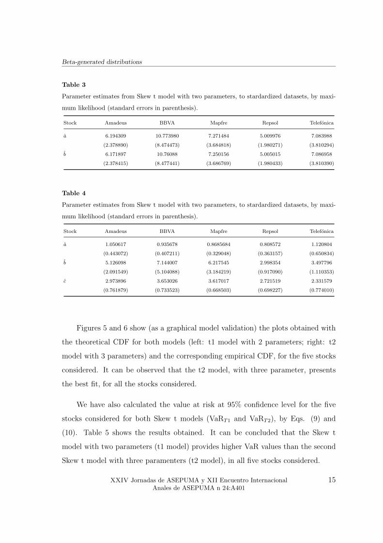
Figures 5 and 6 show (as a graphical model validation) the plots obtained with

the theoretical CDF for both models (left: t1 model with 2 parameters; right: t2

model with 3 parameters) and the corresponding empirical CDF, for the five stocks

considered. It can be observed that the t2 model, with three parameter, presents

the best fit, for all the stocks considered.

We have also calculated the value at risk at 95% confidence level for the five

stocks considered for both Skew t models (VaRT1 and VaRT2), by Eqs. (9) and

(10). Table 5 shows the results obtained. It can be concluded that the Skew t

model with two parameters (t1 model) provides higher VaR values than the second

Skew t model with three paramenters (t2 model), in all five stocks considered.


15


−6 −4 −2 0 2

0.0

0.2

0.4

0.6

0.8

1.0

Amadeus_t1

z

F(z

)

−6 −4 −2 0 2

0.0

0.2

0.4

0.6

0.8

1.0

Amadeus_t2

zF

(z)

−3 −2 −1 0 1 2

0.0

0.2

0.4

0.6

0.8

1.0

BBVA_t1

z

F(z

)

−3 −2 −1 0 1 2

0.0

0.2

0.4

0.6

0.8

1.0

BBVA_t2

z

F(z

)

−4 −2 0 2

0.0

0.2

0.4

0.6

0.8

1.0

Mapfre_t1

z

F(z

)

−4 −2 0 2

0.0

0.2

0.4

0.6

0.8

1.0

Mapfre_t2

z

F(z

)

Figure 5: Plots of the theoretical CDFs of the Skew t models (Left: t1, model with two parameter,

Right: t2, model with three parameters) and the empirical CDF. Stocks: Amadeus; BBVA; Mapfre.


16


−4 −2 0 2

0.0

0.2

0.4

0.6

0.8

1.0

Repsol_t1

z

F(z

)

−4 −2 0 2

0.0

0.2

0.4

0.6

0.8

1.0

Repsol_t2

z

F(z

)

−3 −2 −1 0 1 2 3 4

0.0

0.2

0.4

0.6

0.8

1.0

Telefónica_t1

z

F(z

)

−3 −2 −1 0 1 2 3 4

0.0

0.2

0.4

0.6

0.8

1.0

Telefónica_t2

z

F(z

)

Figure 6: Plots of the theoretical CDFs of the Skew t models (Left: t1 model with two parameter,

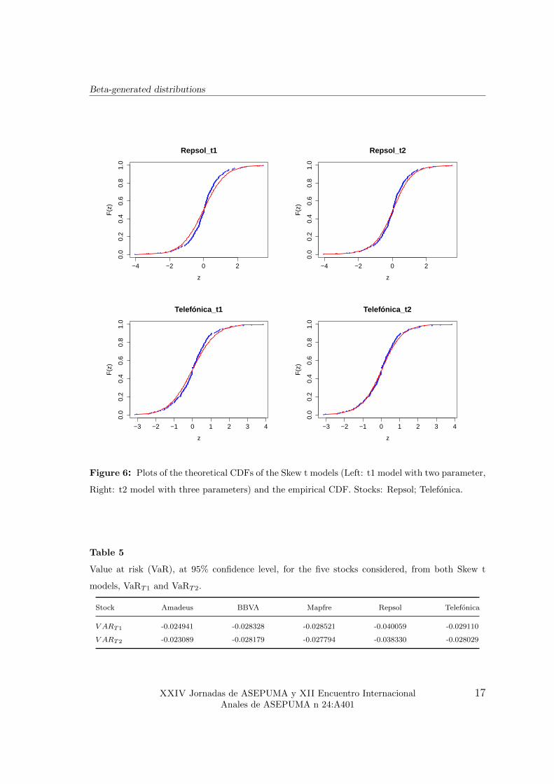
Right: t2 model with three parameters) and the empirical CDF. Stocks: Repsol; Telefonica.

Table 5

Value at risk (VaR), at 95% confidence level, for the five stocks considered, from both Skew t

models, VaRT1 and VaRT2.


V ART1 -0.024941 -0.028328 -0.028521 -0.040059 -0.029110

V ART2 -0.023089 -0.028179 -0.027794 -0.038330 -0.028029


17


7 CONCLUSIONS

In this paper we have proposed the use of some models of beta-generated and

generalized beta-generated distributions (see Eugene et al., 2002 and Jones, 2004),

for modelling financial data. We have studied two classes of skew t distributions,

proposed by Jones and Faddy (2003) and Alexander et al. (2012). The first family

depends on two shape parameters which control the skewness and the tail weight,

and the second family includes an extra parameter. We have obtained analytical ex-

pressions for the cumulative distribution function, quantile function and moments,

and some quantities useful in financial econometrics, including the value at risks,

and we have provided several stochastic representations for these families in terms of

usual distributions functions. We have proposed some multivariate extensions and

we have explored some of their properties. Finally, and empirical application with

real data have been provided.

Acknowledgements. The authors gratefully acknowledge financial support from

the Programa Estatal de Fomento de la Investigacion Cientıfica y Tecnica de Ex-

celencia, Spanish Ministry of Economy and Competitiveness, ECO2013-48326-C2-

2-P. In addition, this work is part of the Research Project APIE 1/2015-17: “New

methods for the empirical analysis of financial markets” of the Santander Financial

Institute (SANFI) of UCEIF Foundation resolved by the University of Cantabria

and funded with sponsorship from Banco Santander.

8 REFERENCES

• ALEXANDER, C., CORDEIRO, G.M., ORTEGA, E.M.M., SARABIA, J.M.

(2012). “Generalized beta-generated distributions”. Computational Statistics

and Data Analysis 56, 1880-1897.


18


• ALEXANDER, C., SARABIA, J.M. (2010). “Generalized beta-generated dis-

tributions”. ICMA Centre Discussion Papers in Finance DP2010-09, ICMA

Centre. The University of Reading, Witheknights, PO Box 242, Reading RG6

6BA, UK.

• AZZALINI, A., CAPITANIO, A. (2003). “Distributions generated by per-

turbation of symmetry with emphasis on a multivariate skew t distribution”.

Journal of the Royal Statistical Society B 65, 367n389.

• BOLLERSLEV, T. (1987). “A conditional heteroskedastic time series model

for speculative prices and rates of return”. Review of Economics and Statistics

69, 542-547.

• CASTILLO, E., HADI, A.S., BALAKRISHNAN , N., SARABIA, J.M. (2005).

“Extreme value and related models with applications in engineering and sci-

ence”. John Wiley & Sons.

• CORDEIRO, G.M., DE CASTRO, M. (2011). “A new family of generalized

distributions”. Journal of Statistical Computation and Simulation, 81, 883-

893.

• EUGENE, N., LEE, C., FAMOYE, F. (2002). “The beta-normal distribution

and its applications”. Communications in Statistics, Theory and Methods, 31,

497-512.

• JONES, M.C. (2004). “Families of distributions arising from distributions of

order statistics”. Test 13, 1-43.

• JONES, M.C., FADDY, M.J. (2003). “A skew extension of the t-distribution,

with applications”. Journal of the Royal Statistical Society. Series B 65,

159-174.


19


• SARABIA, J.M., PRIETO, F., JORDA, V. (2014). “Bivariate Beta-Generated

Distributions with Applications to Well-Being Data”. Journal of Statistical

Distributions and Applications 2014, 1-15.

• SARABIA, J.M., PRIETO, F., JORDA, V., REMUZGO, L. (2016). “Beta-

Generated Distributions with Applications in Finance”. Working Paper, De-

partment of Economics, University of Cantabria.

• SCHWARZ, G. (1978). “Estimating the dimension of a model”. The Annals

of Statistics 5, 461-464.

• THEODOSSIOU, P. (1998). “Financial data and the skewed generalized t

distribution”. Management Science 44, 1650-1661.

• ZHU, D., GALBRAITH, J.W. (2010). “A generalized asymmetric Student-t

distribution with application to financial econometrics”. Journal of Econo-

metrics 157, 297-305.


20

Date post:	27-Jun-2018
Category:	Documents
Upload:	truongdat
View:	223 times
Download:	0 times

Some models of beta-generated distributions with ... · Beta-generated distributions Some models of...

Documents