Some Notes from the Book:

Pairs Trading:

Quantitative Methods and Analysis

by Ganapathy Vidyamurthy

John L. Weatherwax∗

Sept 30, 2004

∗wax@alum.mit.edu

1

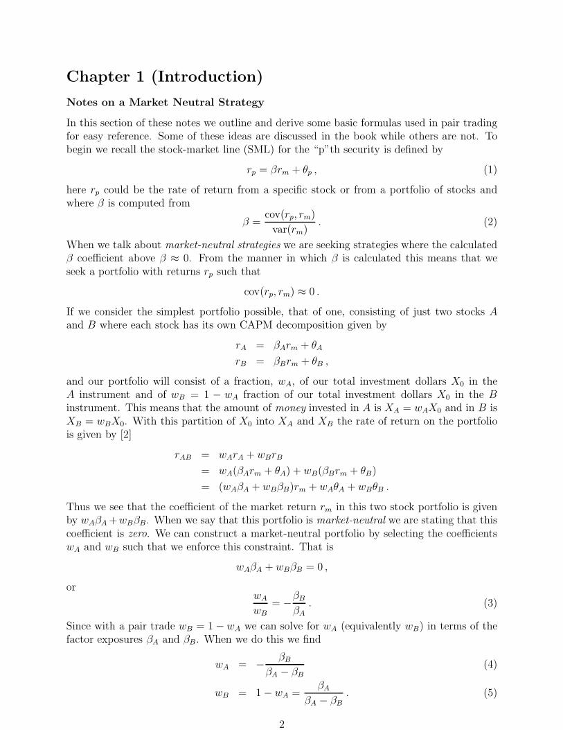
Chapter 1 (Introduction)

Notes on a Market Neutral Strategy

In this section of these notes we outline and derive some basic formulas used in pair tradingfor easy reference. Some of these ideas are discussed in the book while others are not. Tobegin we recall the stock-market line (SML) for the “p”th security is defined by

rp = βrm + θp , (1)

here rp could be the rate of return from a specific stock or from a portfolio of stocks andwhere β is computed from

β =cov(rp, rm)

var(rm). (2)

When we talk about market-neutral strategies we are seeking strategies where the calculatedβ coefficient above β ≈ 0. From the manner in which β is calculated this means that weseek a portfolio with returns rp such that

cov(rp, rm) ≈ 0 .

If we consider the simplest portfolio possible, that of one, consisting of just two stocks Aand B where each stock has its own CAPM decomposition given by

rA = βArm + θA

rB = βBrm + θB ,

and our portfolio will consist of a fraction, wA, of our total investment dollars X0 in theA instrument and of wB = 1 − wA fraction of our total investment dollars X0 in the Binstrument. This means that the amount of money invested in A is XA = wAX0 and in B isXB = wBX0. With this partition of X0 into XA and XB the rate of return on the portfoliois given by [2]

rAB = wArA + wBrB

= wA(βArm + θA) + wB(βBrm + θB)

= (wAβA + wBβB)rm + wAθA + wBθB .

Thus we see that the coefficient of the market return rm in this two stock portfolio is givenby wAβA +wBβB. When we say that this portfolio is market-neutral we are stating that thiscoefficient is zero. We can construct a market-neutral portfolio by selecting the coefficientswA and wB such that we enforce this constraint. That is

wAβA + wBβB = 0 ,

orwA

wB

= −βB

βA

. (3)

Since with a pair trade wB = 1 − wA we can solve for wA (equivalently wB) in terms of thefactor exposures βA and βB. When we do this we find

wA = −βB

βA − βB

(4)

wB = 1 − wA =βA

βA − βB

. (5)

2

Using these formulas we can derive the number of shares to transact in A and B simplyby dividing the dollar amount invested in each by the current price of the security. Theformulas for this are

NA =XA

pA

=wAX0

pA

= −

(

βB

βA − βB

)

X0

pA

(6)

NB =XB

pB

=wBX0

pB

=

(

βA

βA − βB

)

X0

pB

. (7)

This means that given the number of shares we will order for A (or B) to get a market-neutral portfolio are directly related to their factor exposures βA and βB using the aboveformulas. An example MATLAB script that demonstrates some of the equations is given insample portfolio return.m.

3

Chapter 2 (Time Series)

Notes on time series models

See the MATLAB file ts plots.m for code that duplicates the qualitative time series pre-sented in this section of the book. The results of running this code are presented in Figure 1.These plots agree qualitatively with the ones presented in the book.

Notes on model choice (AIC)

In the R file dup figure 2 5.R we present code that duplicates figures 2.5A and 2.5B fromthe book. When this code is run the result is presented in Figure 2. We see the samequalitative figure as in the book, namely that the AIC is minimized with 4 parameters(three AR coefficients and the mean of the time series). While not explicitly stated in thebook, I’m given the understanding that the author feels that the use of the AIC to be veryimportant in selecting the time series model. In fact if a time series is fit using R with thearima command one of the outputs is the AIC. This makes it very easy to use this criterionto select the model we should use to best predict future returns with.

Notes on modeling stock prices

In this subsection of these notes we attempted to duplicate the qualitative behavior of theresults presented in this chapter on modeling stock prices of GE. To do this we extractedapproximately 100 closing prices (data was extracted over the dates from 01/02/2010 to06/04/2010 which yielded 107 data points) and performed the transformation suggested inthis section of the book. This is performed in the R code dup modeling stock prices.R andwhen that script is run we obtain the plots shown in Figure 3. From the plots presented thereit looks like the normal approximation for the returns of GE is a reasonable approximation.The plots in Figure 3 also display the well know facts that the tails of asset returns are notwell modeled by the Gaussian distribution. In fact the returns of GE over this period appearto be very volatile.

4

0 20 40 60 80 100

−3

−2

−1

0

1

2

3

white noise series

0 20 40 60 80 100

−3

−2

−1

0

1

2

3

MA(1) series

0 10 20 30 40 50 60 70 80 90 100−6

−4

−2

0

2

4

6

8AR(1) series

0 10 20 30 40 50 60 70 80 90 100−5

0

5

10

15

20

25

30random walk series

Figure 1: A duplication of the various time series model discussed in this chapter. TopRow: A white noise time series and a MA(1) time series. Bottom Row: An AR(1) timeseries and a random walk time series.

5

0 20 40 60 80 100

−4−2

02

4

AR(3) Series

index

ts v

alue

2 4 6 8 10

7080

9010

011

012

013

0AIC Plot

Number of Parameters

AIC

Val

ue

Figure 2: The AIC for model selection. Left: The time series generated by an AR(3)model. Right: The AIC for models with various orders plotted as a function of parametersestimated.

6

0 20 40 60 80 100

2.75

2.80

2.85

2.90

2.95

GE Series

index

log(

clos

ing

pric

e)

0 20 40 60 80 100

−0.0

6−0

.04

−0.0

20.

000.

020.

040.

06

GE rate of return

index

retu

rns

−2 −1 0 1 2

−0.0

6−0

.04

−0.0

20.

000.

020.

040.

06

Normal Q−Q Plot

Theoretical Quantiles

Sam

ple

Qua

ntile

s

0 5 10 15 20

−0.2

0.0

0.2

0.4

0.6

0.8

1.0

Lag

ACF

Series dlcp

Figure 3: Modeling of the returns of the stock GE. Top Row: The log price time series ofthe closing prices of GE. The first difference of these log prices (the daily returns). BottomRow: A qq-plot of GE daily returns and the autocorrelation function of the returns. Notethat from the qq-plot we see that for “small” returns a normal approximation is quite goodbut that the extreme returns observed don’t fit very well with a normal model. Perhapsoptions on GE were mispriced during this time frame.

7

Chapter 3 (Factor Models)

Notes on arbitrage pricing theory (APT)

We simply note here that given an explicit specification of the k factors we desire to use inour factor model (and correspondingly their returns ri) one can compute the factor expo-sures (β1, β2, · · · , βk) and the idiosyncratic return re simply by using multidimensional linear

regression. Namely we seek a linear model for r using ri as

r = β1r1 + β2r2 + β3r3 + · · · + βkrk + re . (8)

Thus the technique linear regression enables us to determine the factor exposures β andthe idiosyncratic returns re for each stock.

The factor covariance matrix

With the following APT factor decompositions for two instruments A and B

rA =

k∑

i=1

βA,iri + rA,e

rB =k

∑

j=1

βB,jrj + rB,e ,

then we have that the product of the two returns rArB is given by

rArB =

k∑

i=1

k∑

j=1

βA,iβB,jrirj + rA,e

k∑

j=1

βB,jrj + rB,e

k∑

i=1

βA,iri + rA,erB,e .

To compute the covariance of rA and rB we take the expectation of the above expressionand use the facts that

E

[

rA,e

k∑

j=1

βB,jrj

]

= E

[

rB,e

k∑

i=1

βA,iri

]

= E[rA,erB,e] = 0 ,

since rA,e and rB,e are assumed to be zero mean uncorrelated with the factor returns ri, anduncorrelated with idiosyncratic returns from different stocks. Using these facts we concludethat

cov(rA, rB) =k

∑

i=1

k∑

j=1

βA,iβB,jE[rirj]

=[

βA,1 βA,2 · · · βA,k

]

E[r21] E[r1r2] · · · E[r1rk]

E[r2r1] E[r22] · · · E[r2rk]

......

. . ....

E[rkr1] E[rkr2] · · · E[r2k]

βB,1

βB,2...

βB,k

= eAVeTB ,

where eA = (βA,1, βA,2, · · · , βA,k) and eB = (βB,1, βB,2, · · · , βB,k) are the vectors of factorexposures for the A and B-th security respectively and V is the factor covariance matrix.

8

Using a factor model to calculate the risk on a portfolio

Recall that the total return variance on our portfolio is the sum of two parts, a commonfactor variance and a specific variance as

σ2ret = σ2

cf + σ2specific . (9)

Arbitrage pricing theory (APT) tells us that the common factor covariance is computed fromeT

p V ep where ep is the factor exposure profile of the entire portfolio. Thus to evaluate thecommon factor variance for a portfolio we need to be able to compute the factor exposureep for the portfolio. As an example, in the simplest case of a two stock portfolio with a hA

weight in stock A and a hB weight in stock B then we have a factor exposure vector ep givenby the weighted sum of the factor exposure profiles of A and B as

ep = hAeA + hBeB .

Where if we assume a two factor model eA = (βA,1, βA,2) is the factor exposure profile ofstock A and eB = (βB,1, βB,2) is the factor exposure profile of stock B. Using the above, wehave that

ep = (hAβA,1 + hBβB,1, hAβA,2 + hBβB,2)

=[

hA hB

]

[

βA,1 βA,2

βB,1 βB,2

]

= hX .

Where the vector h above is the “holding” or weight vector that contains the weights of eachcomponent A and B as elements and X is the factor exposure matrix.

Notes on the calculation of a portfolios beta

As discussed in the text the optimal hedge ratio λ between our portfolio p and the marketm is given by

λ =cov(rp, rm)

var(rm). (10)

To use APT to compute the numerator in the above expression requires a bit of finesse orat least the expression presented in the book for λ seemed to be a jump in reasoning sincesome of the notation used there seemed to have changed or at least needs some furtherexplanation. We try to elucidate on these points here. In general, the original portfolio pwill consist of a set of equities with a weight vector given by hp. This set of stocks is tobe contrasted with the market portfolio with may consist of stocks that are different thansymbols in the portfolio p. Lets denote the factor exposure matrix of the stocks in theportfolio as Xp which will be of size Np × k and the factor exposure matrix of the market asXm which will be of size Nm × k. Here where Np is the number of stocks in our portfolio,Nm is the number of stocks in the market portfolio, and k is the number of factors in ourfactor model. Note the dimensions of Xm and Xp maybe different. Then using ideas fromthis and the previous section means that the common factors variance σ2

cf can be expressedby multiplying ep = hpXp on the left and em = hmXm on the right of the common factorcovariance matrix V as

σ2cf = hpXpV(hmXm)T = hpXpVXT

mhTm .

9

Now even if the dimensions of Xm and Xp are different the product above still is valid. Thespecific variance σ2

specific needed to evaluate cov(rp, rm) in this case is given by

σ2specific = hp,common∆commonh

Tm,common ,

where ∆common is a diagonal matrix with the specific variances of only the stocks that are incommon to both the original portfolio and the market portfolio. If there are no stocks thatmeet this criterion then this entire term is zero. Another way to evaluate this numerator is tosimply extend the holding vectors of both the portfolio and the market to include all stocksfound in either the original and the market portfolios. In that case the portfolio holdingsvector, hp, would have zeros in places where stocks are in the market but are not in ourportfolio and the market holdings vector, hm, would have zeros in places where there arestocks that are in our portfolio but not in the market portfolio.

Notes on tracking basket design

In this section of these notes we elucidate on the requirements to design a portfolio p that willto track the market m as closely as possible. Using APT to evaluate the variance of rm − rp,we are led to look for a holding vector hp such that minimizes the following expression

var(rm − rp) = var(rm) + var(rp) − 2cov(rm, rp)

= hmXVXThTm + hm∆hT

m (11)

+ hpXVXThTp + hp∆hT

p (12)

− 2(hmXVXThTp + hm∆hT

p ) . (13)

Here the three parts represented by the terms on lines 11, 12 and 13 above are the marketvariance, the tracking basket variance, and the covariance between the market and theportfolio respectively. We can also write this objective function as

var(rm − rp) = hmXVXThTm + hpXVXThT

p − 2hmXVXThTp (14)

+ hm∆hTm + hp∆hT

p − 2hm∆hTp (15)

The terms on lines 14 are the common factor terms and the terms on line 15 are the specificvariance terms. Now it might be hard to optimize this expression directly but we can derivea very useful practical algorithm by recalling that the contribution to the total varianceform the common factor terms on line 14 is normally much larger in magnitude than thecontribution to the total variance from the specific terms on line 15. Thus making thecommon factor terms as small as possible will be more important and make more of animpact in the total minimization than making the specific variance terms small.

With this motivation, observe that if we select a portfolio holding vector hp, such that

hpX = hmX , (16)

then the combination of the three terms hmXVXThTm, hpXVXThT

p and −2hmXVXThTp on

line 14 vanish (leaving a zero common variance) and we are left with the following minimumvariance portfolio design criterion

minhp:hpX=hmX

(hm∆hTm + hp∆hp − 2hm∆hT

p ) .

10

This remaining problem is a quadratic programming problem with linear constraints. As apractical matter we will often be happy (and consider the optimization problem solved) whenwe have specified a portfolio that satisfies hpX = hmX. As a notational comment, since thedefinition of the factor exposures of the portfolio and the market are given by ep = hpX andem = hmX the statement made by Equation 16 is that the factor exposures of the trackingportfolio should equal the factor exposures of the market.

If the specific factors selected for the columns of X are actual tradable instruments thenthe criterion hmX = hpX, explicitly states how to optimally hedge the given portfolio, p, sothat it will be market neutral. To see this note that the holding vector hp has components,hi,p, that represent the percent of money held in the ith equity. If we multiply the portfolioholding vector hp by the dollar value of the portfolio D we get

Dhp = (Dh1,p, Dh2,p, Dh3,p, · · · , DhN,p) = (N1p1, N2p2, N3p3, · · · , NNpN) ,

where Ni and pi represents the number of shares and current price of the ith security and thereare N total securities in our universe. If the columns of our factor exposure matrix representactual tradable instruments, then each component of the row vector DhpX represents the

exposure to the given security (factor). If the elements of X are β(j)i we can write the jth

component of the product DhpX (representing the exposure of this portfolio to the j factor)as

(DhpX)j =

N∑

i=1

Nipiβ(j)i ,

for 1 ≤ j ≤ k where k is the number of factors. Using hpX = hmX, since the factors areactually tradables it is easy to find a market holding vector that will equal the above sum. Ifwe do this the combined holdings of the original portfolio and the newly constructed marketportfolio will be market neutral and will have a very small variance.

For example, assume we have only three factors k = 3 and we take as the market holdingvector hm a vector of all zeros except for the three elements that correspond to the tradablefactors. If these three tradable factors are located at the indices i1, i2 and i3 among all ofour N tradable securities then we get for the jth component of DhmX

(DhmX)j = D

N∑

i=1

hi,mβ(j)i = D(hi1,mβ

(j)i1

+ hi2,mβ(j)i2

+ hi3,mβ(j)i3

)

= Ni1pi1β(j)i1

+ Ni2pi2β(j)i2

+ Ni3pi3β(j)i3

.

Here Nij is the number of shares in the jth factor and specifying its value is equivalent tospecifying the non-zero components of hm, and pij is the current price of the j factor. If wewrite out DhpX = DhmX for the three factors j = 1, 2, 3 we get three linear equations.

N∑

i=1

Nipiβ(1)i = Ni1pi1β

(1)i1

+ Ni2pi2β(1)i2

+ Ni3pi3β(1)i3

N∑

i=1

Nipiβ(2)i = Ni1pi1β

(2)i1

+ Ni2pi2β(2)i2

+ Ni3pi3β(2)i3

N∑

i=1

Nipiβ(3)i = Ni1pi1β

(3)i1

+ Ni2pi2β(3)i2

+ Ni3pi3β(3)i3

.

11

Since each of the given factors is a tradable we expect that the β values above will be 1 or0. This is because when we do the factor regression

ri1 =k

∑

j=1

β(j)i1

ri + ǫi1

on the i1 security the only non-zero β is the one for the i1 security itself and its value is 1.Thus the system above decouples into three scalar equations

N∑

i=1

Nipiβ(1)i = Ni1pi1

N∑

i=1

Nipiβ(2)i = Ni2pi2

N∑

i=1

Nipiβ(3)i = Ni3pi3 ,

for the unknown values of Ni1 , Ni2 and Ni3 . These are easily solved. Buying a portfolioof the hedge instruments in share quantities with signs opposite that of Ni1 , Ni2 and Ni3

computed above will produced a market neutral portfolio and is the optimal hedge.As a very simple application of this theory we consider a single factor model where the

only factor is the underlying market and a portfolio with only a single stock A. We assumewe have NA shares, the stock is trading at the price pA, and has a market exposure of βA.We then ask what the optimal number of shares NB of a stock B, trading at pB and witha market exposure of βB, we would need to order so that the combined portfolio is marketneutral. Using the above equations we have

NApAβA = NBpBβB so NB =βApA

βBpB

NA .

Thus we would need to sell NB shares to get a market neutral portfolio. This is the sameresult we would get from Equation 7 (with a different sign) when we replace X0 with whatwe get from Equation 6. The fact that the sign is different is simply a consequence of theconventions used when setting up each problem.

12

Chapter 4 (Kalman Filtering)

Notes on the text

A very nice book, that goes into Kalman filtering in much more detail is [1].

the scalar Kalman filter: optimal estimation with two measurements of a con-stant value

In this section of these notes we provide an alternative an almost first principles derivationof how to combine two estimate of an unknown constant x. In this example here we assumethat we have two scalar measurements yi of the scalar x each with a different uncertaintyσ2

i . Namely,zi = x + vi with vi ∼ N(0, σ2

i ) .

To make these results match the notation in the book the first measurement z1 correspondsto the a priori estimate xi|i with uncertainty σ2

ε,i and the second measurement z2 correspondsto yi with uncertainty σ2

η,i. We desire our estimate x of x to be a linear combination of thetwo measurements zi for i = 1, 2. Thus we take x = k1z1 + k2z2, and define x to be ourestimate error given by x = x−x. To make our estimate x unbiased requires we set E[x] = 0or

E[x] = E[k1(x + v1) + k2(x + v2) − x] = 0

= E[(k1 + k2)x + k1v1 + k2v2 − x]

= E[(k1 + k2 − 1)x + k1v1 + k2v2]

= (k1 + k2)x − x = (k1 + k2 − 1)x = 0 ,

thus this requirement becomes k2 = 1 − k1 which is the same as the books Equation 1.0-4.Next lets pick k1 and k2 (subject to the above constraint such that) the error as small aspossible. When we take k2 = 1 − k1 we find that x is given by

x = k1z1 + (1 − k1)z2 ,

so x is given by

x = x − x = k1z1 + (1 − k1)z2 − x

= k1(x + v1) + (1 − k1)(x + v2) − x

= k1v1 + (1 − k1)v2 . (17)

Next we compute the expected error or E[x2] and find

E[x2] = E[k21v

21 + 2k1(1 − k1)v1v2 + (1 − k1)

2v22]

= k21σ

21 + 2k1(1 − k1)E[v1v2] + (1 − k1)

2σ22

= k21σ

21 + (1 − k1)

2σ22 ,

since E[v1v2] = 0 as v1 and v2 are assumed to be uncorrelated. This is the books equation 1.0-5. We desire to minimize this expression with respect to the variable k1. Taking its derivativewith respect to k1, setting the result equal to zero, and solving for k1 gives

2k1σ21 + 2(1 − k1)(−1)σ2

2 = 0 ⇒ k1 =σ2

2

σ21 + σ2

2

.

13

Putting this value in our expression for E[x2] to see what our minimum error is given by wefind

E[x2] =

(

σ22

σ21 + σ2

2

)2

σ21 +

(

σ21

σ21 + σ2

2

)2

σ22

=σ2

1σ22

(σ21 + σ2

2)2

(

σ22 + σ2

1

)

=σ2

1σ22

(σ21 + σ2

2)

=1

1σ21

+ 1σ22

=

(

1

σ21

+1

σ22

)−1

,

which is the books equation 1.06. Then our optimal estimate x take the following form

x =

(

σ22

σ21 + σ2

2

)

z1 +

(

σ21

σ21 + σ2

2

)

z2 .

Some special cases of the above that validate its usefulness are when each measurementcontributes the same uncertainty then σ1 = σ2 and we see that x = 1

2z1 + 1

2z2, or the average

of the two measurements. As another special case if one measurement is exact i.e. σ1 = 0,then we have x = z1 (in the same way if σ2 = 0, then x = z2). These formulas all agree withsimilar ones in the text.

Notes on the filtering the random walk

In this section of these notes we consider measurements and dynamics of a security asit undergoes the random walk model. To begin, we write the sequence of measurement,state propagation, measurement, state propagation over and over again until we reach thediscrete time t where we wish to make an optimal state estimate denoted xt. Denotingthe measurements by yt and true states by xt this discrete sequence of equations under therandom walk looks like

y0 = x0 + e0 0th measurement

x1 = x0 + ε1 propagation

y1 = x1 + e1 1st measurement

x2 = x1 + ε2 propagation

y2 = x2 + e2 2nd measurement

x3 = x2 + ε3 propagation

y3 = x3 + e3 3rd measurement

x4 = x3 + ε4 propagation...

yt−1 = xt−1 + et−1 ”t − 1”th measurement

xt = xt−1 + εt propagation

yt = xt + et our final measurement.

Here xt is the log-price and y is a measurement of the “fair” log-price both at time t. Now wewill use all of the above information to estimate the value of xt (and actually xl for l ≤ t).From the above system we observe that we have t + 1 unknowns x0, x1, · · · , xt and t + 1

14

measurements y0, y1, · · · , yt but only 2t + 1 equations. To estimate the values of xt for allt we can use the method of least squares. When et and εt come from a zero-mean normaldistribution with equal variances this procedure corresponds to ordinary least squares. Ifet and εt are have different variances we need to use the method of weighted least squares.To complete this discussion we assume that the process noise and the measurement noiseare the same so that we can use ordinary least squares and then write the above system asthe matrix system

y0

0y1

0y2

0y3

0...

yt−1

0yt

=

1 0 0 0 0 0−1 1 0 0 00 1 0 0 00 −1 1 0 00 0 1 0 00 0 −1 1 00 0 0 1 00 0 0 −1 1...

. . .. . .

. . ....

0 1 00 −1 1

0 0 0 1

x0

x1

x2

x3

x4...

xt−1

xt

+

e0

−ε1

e1

−ε2

e2

−ε3

e3

−ε4...

et−1

−εt

et

.

Here the pattern of the coefficient matrix in front of the vector of unknowns, denoted by H ,

is constructed from several blocks like

[

1 0−1 1

]

, placed on top of each other but translated

one unit to the right. This matrix can be created for any integer value of t using theMATLAB function create H matrix.m. Once we have the H matrix the standard leastsquare estimate of the vector x is obtained by computing x = (HTH)−1HT y, where y is thevector left-hand-side in the above matrix system. Since the y vector has zeros at every otherlocation these zeros make the numerical values in the corresponding columns of the productmatrix (HTH)−1HT irrelevant since their multiplication is always zero. Thus the result ofthe product of (HTH)−1HT and the full y is same as the action of the matrix (HT H)−1HT

with these zero index columns removed on the vector y again with the zeros removed. Thusthe discussed procedure for estimating x is very inefficient since all the computations involvedin computing the unneeded columns are unnecessary. An example to clarify this may help.If we take t = 2 in the above expressions and compute (HT H)−1HT we get the matrix

5/8 -3/8 1/4 -1/8 1/8

1/4 1/4 1/2 -1/4 1/4

1/8 1/8 1/4 3/8 5/8

Now y when t = 2 in this case is given by

y =

y0

0y1

0y2

.

15

Then due to the zeros in the vector y the product x = (HT H)−1HTy is equivalent to thesimpler product

x0

x1

x2

=

5/8 1/4 1/81/4 1/2 1/41/8 1/4 5/8

y0

y1

y2

.

If we express the above matrix product as a sequence of scalar equations we have

x0 =5

8y0 +

1

4y1 +

1

8y2

x1 =1

4y0 +

1

2y1 +

1

4y2

x2 =1

8y0 +

1

4y1 +

5

8y2 .

Note that this formulation gives us estimates of all components of x and that the estimates ofdata points earlier in time depend on measurements later in time making them not practicalfor a fully causal algorithm (smoothing is a possibility however). From the above we see thatthe optimal estimate of x2 is given by

x2 =1

8y0 +

1

4y1 +

5

8y2 ,

this agrees with the result in the book. Thus the elements of (HT H)−1HT eventually becomeweights to which we multiply the individual measurements yi. When we take t = 3 andremove the columns (HT H)−1HT corresponding to the zero elements of y we get a matrixof weights

x =

13/21 5/21 2/21 1/215/21 10/21 4/21 2/212/21 4/21 10/21 5/211/21 2/21 5/21 13/21

y ,

where y has the same elements of y but with the zeros removed. Performing one moreexample, when we take t = 4 and remove the columns (HTH)−1HT corresponding to thezero elements of y we get a matrix of weights

x =

34/55 13/55 1/11 2/55 1/5513/55 26/55 2/11 4/55 2/551/11 2/11 5/11 2/11 1/112/55 4/55 2/11 26/55 13/551/55 2/55 1/11 13/55 34/55

y .

See the MATLAB file equal variance kalman weights.m where we calculate these matri-ces. The weights used to optimally estimate xt are given by the last row in the above twomatrices. Thus as we add samples the amount of computation needed to estimate xt in thismanner increases. The reformulation of this least squares estimation of xt into a recursive

algorithm that avoids forming these matrices and requiring all of this work is one of thebenefits obtained when using the time domain Kalman filtering framework.

If we recognize from the examples above that the effect in the estimate of xt on observedpast data points decays rather quickly and since the probability distributions above arestationary (i.e. don’t depend on the time index), we would expect that we could pick a value

16

of t, form the matrix (HTH)−1HT once to compute a set of constant weights and simplyuse these weights into the future. It can be shown that for a general time t the weight wi toapply to yi in the approximation

xt = w0yt + w1yt−1 + w2yt−2 + · · ·+ wt−1y1 + wty0 , (18)

are given by

(w0, w1, w2, · · · , wt−1, wt) =

(

F2(t+1)−1

F2(t+1)

,F2(t+1)−3

F2(t+1)

,F2(t+1)−5

F2(t+1)

, · · · ,F3

F2(t+1)

,F1

F2(t+1)

)

.

If we let t → ∞ these weights go to

(w0, w1, w2, · · · , wt−1, wt) =

(

1

g,

1

g3,

1

g5, · · · ,

1

g2t−1,

1

g2t+1

)

,

where g = 1+√

52

≈ 1.6180 is the golden ratio. If we filter under the assumption of large t wecan save a great deal of computation by avoiding the entire computation of (HT H)−1HT yand simply using these golden ratio based (and fixed) weights. This will be explored in thenext section.

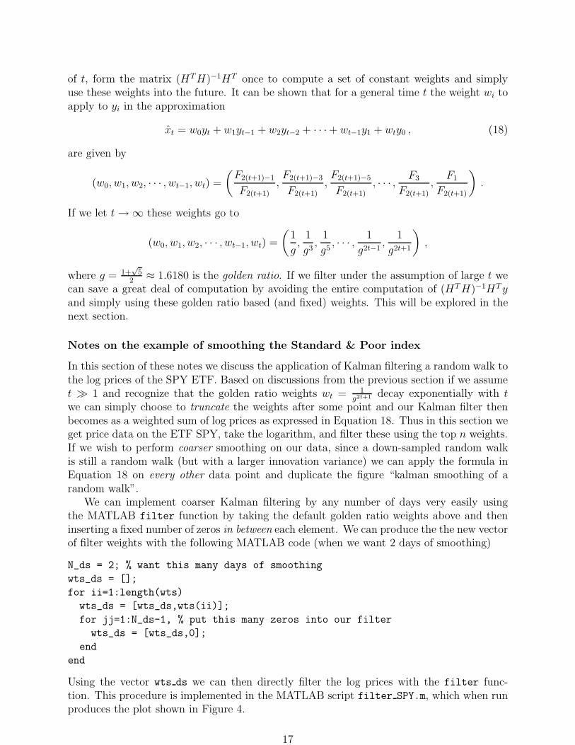
Notes on the example of smoothing the Standard & Poor index

In this section of these notes we discuss the application of Kalman filtering a random walk tothe log prices of the SPY ETF. Based on discussions from the previous section if we assumet ≫ 1 and recognize that the golden ratio weights wt = 1

g2t+1 decay exponentially with twe can simply choose to truncate the weights after some point and our Kalman filter thenbecomes as a weighted sum of log prices as expressed in Equation 18. Thus in this section weget price data on the ETF SPY, take the logarithm, and filter these using the top n weights.If we wish to perform coarser smoothing on our data, since a down-sampled random walkis still a random walk (but with a larger innovation variance) we can apply the formula inEquation 18 on every other data point and duplicate the figure “kalman smoothing of arandom walk”.

We can implement coarser Kalman filtering by any number of days very easily usingthe MATLAB filter function by taking the default golden ratio weights above and theninserting a fixed number of zeros in between each element. We can produce the the new vectorof filter weights with the following MATLAB code (when we want 2 days of smoothing)

N_ds = 2; % want this many days of smoothing

wts_ds = [];

for ii=1:length(wts)

wts_ds = [wts_ds,wts(ii)];

for jj=1:N_ds-1, % put this many zeros into our filter

wts_ds = [wts_ds,0];

end

end

Using the vector wts ds we can then directly filter the log prices with the filter func-tion. This procedure is implemented in the MATLAB script filter SPY.m, which when runproduces the plot shown in Figure 4.

17

20 40 60 80 100 120 140

4.6

4.65

4.7

4.75

4.8

4.85

Days from 20100104

Lo

g o

f d

aily

clo

se

of

SP

Y

log close SPY pricestwo day Kalman smooth

Figure 4: A duplication of the random walk smoothing of SPY using the simplest Kalman fil-ter model. How the MATLAB filter function process data results in the initial discrepancybetween the log prices and the filtered values.

18

Chapter 5 (Overview)

Notes on cointegration: the error correction representation

As a link to the real world of tradables it is instructive to note that the nonstationary seriesxt and yt that we hope are cointegrated and that we will trade based on the signal of are thelog-prices of the A and B securities

xt = log(pAt ) (19)

yt = log(pBt ) . (20)

Under this realization the error correction representation of cointegration given by

xt − xt−1 = αx(xt−1 − γyt−1) + εxt

yt − yt−1 = αy(xt−1 − γyt−1) + εyt,

is a statement that the two returns of the securities A and B are linked via the stationaryerror correction term xt−1 − γyt−1. This series is so important it is given a special name andcalled the spread. Notice that in the error correction representation spread series affects thereturn of A and B via the coefficients αx and αy called the error correction rates for xt andyt. In fact we must have αx < 0 and αy > 0 (see the Matlab script cointegration sim.m).The fact that it should be stationary might give a possible way to find the γ parameter incointegration. Simply use stationarity tests on the spread time series for various values of γin some range and pick the value of γ that makes the spread series “most” stationary. Weexpect that the spread time series to reach some “long run equilibrium” which is to meanthat xt − γyt oscillates about a mean value µ or

xt − γyt ∼ µ as t → ∞ .

If we can take the approximation above as an equality we see that using Equations 19 and 20give

log(pAt ) − γ log(pB

t ) = µ ,

or solving for pBt in terms of pA

t we find

pAt = eµ(pB

t )γ , (21)

is the long run price relationship. The error correction representation is very easy to sim-ulate. In the MATLAB function cointegration sim.m we duplicate the books figures oncointegration. When that code is run it generates plots as shown in Figure 5.

Notes on cointegration: the common trends model

Another characterization of cointegration is the so called common trends model, alsoknown as the Stock-Watson characterization where the two series we assume are cointe-grated are represented as

xt = nxt+ εxt

yt = nyt+ εyt

.

19

0 20 40 60 80 100 120 140 160 180 200−14

−12

−10

−8

−6

−4

−2

0

2

4

6Cointegrated Time Series

xt

yt

0 20 40 60 80 100 120 140 160 180 200−5

−4

−3

−2

−1

0

1

2

3

4

5The Spread of Two Cointegrated Time Series

Figure 5: A demonstration of two cointegrated series. See the text for details.

20

In this formulation, to have the above equations represent prices in our tradable universethe series xt is the given stocks log-price i.e. xt = log

(

pAt

)

, which we have been assuming isa nonstationary random walk like term, the series nxt

is the nonstationary common factor“log-price” (such that the first difference of nxt

is the common factor return), and εxtis the

idiosyncratic log-price (again such that the first difference of εxtis the idiosyncratic return)

which we assume is stationary. If we desire that some linear combination of xt and yt be afully stationary series when we compute xt − γyt we find

xt − γyt = (nxt− γnyt

) + (εxt− γεyt

) .

Thus to be stationary means that we require

nxt− γnyt

= 0 , (22)

or in terms of prices that the common factor log-prices are the same up to a proportionalityconstant γ. This condition is a bit hard to work with and we will see simplified criterionbelow.

Notes on applying the cointegration model

In this section of these note we make some comments on how to apply the theory of cointe-gration to trade pairs of stocks. As a first step we select a pair of stocks to potentially tradeand compute the cointegration coefficient γ for that pair. Methods to select pairs to tradewill be discussed in the following chapter on Page 23. Then we trade based on the value ofthe spread given by

spreadt = log(pAt ) − γ log(pB

t ) . (23)

When this spread is at a “historically” large value (of either sign) we construct a portfolioto take advantage of the fact that we expect the value of this expression to mean revert. Ifwe consider a portfolio p long one share of A and short γ shares of B then the return on thisportfolio from time t to t + i is given by

log

(

pAt+i

pAt

)

− γ log

(

pBt+i

pBt

)

= log(pAt+i) − log(pA

t ) − γ(log(pBt+i) − log(pB

t ))

= log(pAt+i) − γ log(pB

t+i) − (log(pAt ) − γ log(pB

t ))

= spreadt+i − spreadt .

From this expression we see that to maximize the return on this pair portfolio we wait untilthe time t when the value of spreadt is “as small as possible” i.e. less that µ − nl,entry∆,the mean spread, µ, minus some number, nl,entry, of spread standard deviations ∆. We getout of the trade at the time t + i when the value of spreadt+i is “as large as possible” i.e.larger than µ+nl,exit∆, for some other number, nl,exit. The pairs trading strategy is thensummarized as

• If we find at the current time t that

spreadt < µ − nl,entry∆ , (24)

we buy shares in A and sell shares in B in the ratio of NA: NB = 1: γ, and wait to exitthe trade at a time t + i when

spreadt+i > µ + nl,exit∆ . (25)

Here nl,entry and nl,exit are long spread entry and exit threshold parameters respectivly.

21

• If instead we find at the current time t that

spreadt > µ + ns,entry∆ , (26)

we do the opposite trade. That is, we sell shares in A and buy shares in B in the ratioNA: NB = 1: γ, and wait to exit the trade until the time t + i when

spreadt+i < µ − ns,exit∆ . (27)

Here ns,entry and ns,exit are short spread entry and exit threshold parameters respectivly.

Now if we buy NA shares of A and NB shares of B in the ratio 1: γ i.e. NA: NB = 1: γ thismeans that we require

NA

NB

=1

γ, (28)

orNB = γNA . (29)

Using these same ideas, we can also determine a spread based stop loss in a similar manner.For example, if at the time t we determine via Equation 24 that we would like to be long aunit of spread, then by picking a stop loss spread threshold, nsl, at the point we enter thetrade we can evaulate the value of

spreadt − nsl∆ .

If at any point during the trade of this spread unit if the current spread value falls below

this value i.e. spreadt+i < spreadt − nsl∆, we should assume that the spread is not meanreverting and exit the trade.

22

Chapter 6 (Pairs Selection in the Equity Markets)

Notes on the distance measure

The distance measure we will consider is the absolute value of the correlation between thecommon factor returns of two securities which can be written as

d(A, B) = |ρ| =

∣

∣

∣

∣

∣

cov(rA, rB)√

var(rA)var(rB)

∣

∣

∣

∣

∣

.

Since we want to measure only the common factor return we should really write cov(·, ·) andvar(·) with a cf subscript to represent that we only want the common factor variance of thereturn as varcf . From arbitrage pricing theory (APT) can write the above distance measurein terms of the factor exposures eA, eB of our two securities, and the factor covariance matrixV as

|ρ| =

∣

∣

∣

∣

∣

eAVeTB

√

(eAVeTA)(eBVeT

B)

∣

∣

∣

∣

∣

. (30)

The book uses the notation x rather then e to denote the common factor exposure vectorsand F rather than V to denote the common factor covariance matrix. The notation in thisrespect seems to be a bit inconsistent.

Reconciling theory and practice: stationarity of integrated specific returns

From this small subsection of the book we can take away the idea that for pair trading asdiscussed in this book we will do two things

• Consider as a possible pair for trading any two stocks that have a large value of |ρ|(defined above) and for any such pairs estimate their cointegration coefficient γ.

• Using this estimated value of γ, form the spread time series defined by

log(pAt ) − γ log(pB

t ) ,

and test to see if it is stationary.

• If this pair is found to have a stationary spread, we can trade when the spread isobserved to deviate significantly from its long run equilibrium value (denoted here asµ).

Notes on reconciling theory and practice: a numerical example

To test some of these ideas I implemented in the python codes

• find possible pairs.py and

• multifactor stats.py

a multifactor sector based pair searching strategy using the discussed pair statistics. Someof the pairs that these routines found are shown here:

23

sector= Basic Materials with 710 members

Pair: ( RTP, BHP): corr_ii_jj= 0.996833 SNR= 10.390647

Pair: ( RTP, VALE): corr_ii_jj= 0.991511 SNR= 7.247113

Pair: ( BHP, VALE): corr_ii_jj= 0.990573 SNR= 6.922419

sector= Technology with 927 members

Pair: ( AAPL, MSFT): corr_ii_jj= 0.981468 SNR= 5.193737

Pair: ( MSFT, IBM): corr_ii_jj= 0.962065 SNR= 3.522831

Pair: ( AAPL, IBM): corr_ii_jj= 0.892878 SNR= 1.908111

sector= Consumer, Cyclical with 1168 members

Pair: ( TM, MCD): corr_ii_jj= 0.993515 SNR= 12.124917

Pair: ( TM, WMT): corr_ii_jj= 0.986572 SNR= 9.832299

Pair: ( MCD, WMT): corr_ii_jj= 0.975303 SNR= 7.163039

sector= Industrial with 1452 members

Pair: ( GE, UTX): corr_ii_jj= 0.998224 SNR= 10.762886

Pair: ( SI, GE): corr_ii_jj= 0.993410 SNR= 6.432623

Pair: ( SI, UTX): corr_ii_jj= 0.989422 SNR= 5.185361

sector= Funds with 1056 members

Pair: ( EEM, SPY): corr_ii_jj= 0.997625 SNR= 5.831888

Pair: ( EEM, GLD): corr_ii_jj= -0.044805 SNR= 0.430726

Pair: ( SPY, GLD): corr_ii_jj= 0.012789 SNR= 0.080389

sector= Financial with 2851 members

Pair: ( WFC, JPM): corr_ii_jj= 0.997321 SNR= 10.498293

Pair: ( WFC, HBC): corr_ii_jj= 0.989763 SNR= 5.273780

Pair: ( JPM, HBC): corr_ii_jj= 0.981574 SNR= 4.118802

sector= Energy with 879 members

Pair: ( CVX, XOM): corr_ii_jj= 0.986020 SNR= 4.198963

Pair: ( BP, XOM): corr_ii_jj= 0.962390 SNR= 6.936206

Pair: ( BP, CVX): corr_ii_jj= 0.933948 SNR= 5.281772

sector= Diversified with 158 members

Pair: ( LUK, IEP): corr_ii_jj= 0.783188 SNR= 3.222232

Pair: ( IEP, LIA): corr_ii_jj= 0.770306 SNR= 7.884407

Pair: ( LUK, LIA): corr_ii_jj= 0.410682 SNR= 2.619646

sector= Communications with 1354 members

Pair: ( VOD, CHL): corr_ii_jj= 0.992050 SNR= 12.187919

Pair: ( T, CHL): corr_ii_jj= 0.933453 SNR= 3.955416

Pair: ( VOD, T): corr_ii_jj= 0.924183 SNR= 3.067509

24

These pairs look like a representative selection of stocks one would consider to possiblybe cointegrated. Since the multifactor pairs searching strategy is quite time intensive weperform this procedure rather infrequently (once a month).

25

Chapter 7 (Testing for Tradability)

Notes on estimating the linear relationship: various approaches

This section of the book seems to be concerned with various ways to estimate the parametersγ and µ in the definition of the spread time series given by Equation 23. The book proposesthree methods: the multifactor approach, the minimizing chi-squared approach, and theregression approach. Here I summarize these methods in some detail. Note that in each ex-pression, the parameters we are estimating could have a subscript to denote the independentvariable. For example, in estimating γ we could call it γAB since we are assuming that theB log prices of the stock is the independent variable. An expression for γBA can be obtainedby exchanging A and B in the formulas given. In general, we will compute both expressionsthat is γAB and γBA and fix the (A, B) ordering for our stocks to enforce γAB > γBA. Thevarious approaches for estimate the statistics of the spread time series st are

• Multifactor approach: This method is based on the decomposition of each stocksreturn into factor returns and factor uncertainties. Given the common factor covari-ance matrix, F, and each stocks factor exposure vectors eA and eB, the cointegrationcoefficient γ under the method is given by

γ =eT

AFeB

eTBFeB

.

An expression for µ is obtained by computing the mean of the spread time series. Thismethod is implemented in the routine multifactor stats.py.

• Chi-squared approach: In this approach we pick the values of γ and µ to minimizea chi-squared merit function given by

χ2(γ, µ) =N

∑

t=1

(log(pAt ) − γ log(pB

t ) − µ)2

var(εAt ) + γ2var(εB

t ). (31)

Here var(εAt ) are variances of the errors in the observations of log(pA

t ), the same forvar(εB

t ). When dealing with daily data we can estimate var(εAt ) by assuming a uniform

distribution between the low and the highest prices for that day and using the varianceof a uniform distribution given by

var(εAt ) =

1

12(log(pA,high

t ) − log(pA,lowt )) .

To implement the minimization of χ2 many optimization routines require the derivativeof the objective function they seek to minimize with respect to the variables they areminimizing over, which in this case are (γ, µ). So that we have these derivativesdocumented we derive them here. To evaluate these derivatives we define the residualrt and total variance vt time series as

rt ≡ log(pAt ) − γ log(pB

t ) − µ

vt ≡ var(εAt ) + γ2var(εB

t ) .

26

Using these we find

χ2(γ, µ) =N

∑

t=1

rt2

vt

∂χ2(γ, µ)

∂µ= −2

N∑

t=1

rt

vt

∂χ2(γ, µ)

∂γ=

N∑

t=1

(

2rt

vt

∂rt

∂γ−

r2t

v2t

∂vt

∂γ

)

= −2N

∑

t=1

(

rt

vt

log(pBt ) + γ

r2t

v2t

var(εBt )

)

.

This method is implemented in chisquared minimization stats.py.

• Regression approach: This method is the most direct and is based on estimating(γ, µ) from the linear model

log(pAt ) = γ log(pB

t ) + µ .

This method is implemented in the python code linear regression stats.py.

All of these routines are called from the function extract all spread stats.

Notes on testing the residual for tradability

After the initial selection of potential pairs to trade is made, one needs to construct thespread time series given by Equation 23 and test it for tradability. In the best of cases thespread time series will be composed of a mean offset µ and a mean-reverting error term εt

aslog(pA

t ) − γ log(pBt ) = µ + εt .

Once can easily compute the spread time series and subtract its mean to obtain just the timeseries of εt. To have the residual series εt be mean reverting means that this series shouldhave a large number of zero-crossings. One way to get a single estimate of the zero-crossingrate is using

zcr =1

T − 1

T−1∑

t=1

I{spreadtspreadt−1 < 0} , (32)

where spreadt is our demeaned spread signal of length T and the indicator function I{A}is 1 if the argument A is true and 0 otherwise. This is implemented in the python codeestimate zero crossing rate.py. All things being equal we prefer residual series witha large zero-crossing rate, since in that case we don’t have to wait long once we put ona trade for convergence. The book argues that this single point estimate will be heavilybiased towards the particular spread time series under consideration and that a bootstraptechnique should instead be used to estimate the time between zero-crossings. This is donein estimate time between zero crossings.py. Once the time between zero-crossing hasbeen computed for each pair we sort the pairs so that the pairs with the shortest timebetween zero-crossings are presented for potential trading first.

27

Chapter 8 (Trading Design)

Notes on band design for white noise

In this section of these notes we duplicate several of the results presented in the bookwith the MATLAB command white noise band design.m. When this script is run theresults it produces are presented in Figure 6. To begin with we first reconstruct the exactprofit value function ∆(1 − N(∆)) where N(·) is the cumulative density function for thestandard normal. This is plotted in Figure 6 (top). Next, we simulate a white noise randomprocess and estimate the probability that a sample from it has a value greater than ∆. Thisprobability as a function of ∆ is plotted in Figure 6 (middle). Finally, using the aboveestimated probability function we multiply by ∆ to obtain the sample based estimate ofthe profit function. A vertical line is drawn at the location of the empirically estimatedprofit function maximum. These results agree with the ones presented in the book. Apython implementation of the count based probability estimator is given in the functionestimate probability discrete counts.py.

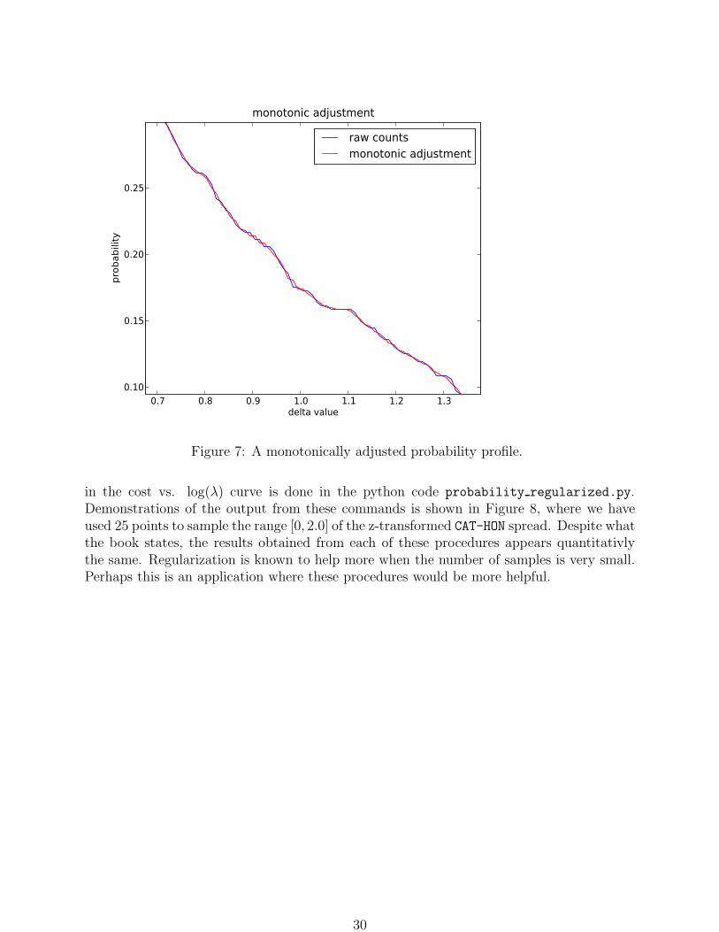
Notes on regularization

The book then presents two functions to more optimally estimate the probability a sampleof the spread st crosses a certain number of sigma away from the mean given the raw countbased estimate. The first is a simple monotonic adjustment of the probability curve andis implemented in the python code probability monotonic adjustment.py. An examplecount based probability curve estimate and the resulting monotonically adjusted probabilityestimate can be seen in Figure 7. The second adjustment is based on imposing a penaltyfor non-smooth functions. This penalty is obtained by adding to the least-squares costfunction an objective function that is larger for sample estimates that are non-smooth andthen minimizing this combined cost function. The book suggests the following cost function

cost(z;y) = (y1 − z1)2 + (y2 − z2)

2 + · · ·+ (yn − zn)2

+ λ[

(z1 − z2)2 + (z2 − z3)

2 + · · ·+ (zn−1 − zn)2]

, (33)

where yi are the monotonically smoothed probability estimates and zi are the smoothnessregularized probability estimates obtained by minimizing the above cost function over z. Asmany optimization routines require the derivative of the cost function they seek to minimizewe find the derivatives of cost(z;y) with respect to z as follows. For i = 1 (the first sample)

∂cost(z;y)

∂z1= −2(y1 − z1) + 2λ(z1 − z2) .

for 2 ≤ i ≤ n − 1

∂cost(z;y)

∂zi

= −2(yi − zi) + 2λ(zi − zi+1) − 2λ(zi−1 − zi) ,

and finally for the last sample i = n

∂cost(z;y)

∂zn

= −2(yn − zn) − 2λ(zn−1 − zn) .

The process of selecting a grid of λ values, minimizing the above cost function as a functionof z and selecting the final estimate of z to be the one that gives the location of the “heel”

28

0 0.2 0.4 0.6 0.8 1 1.2 1.4 1.6 1.8 20

0.02

0.04

0.06

0.08

0.1

0.12

0.14

0.16

0.18White Noise Threshold Design

Amount of Sigma away from the Mean

Profi

t Valu

e

0 0.2 0.4 0.6 0.8 1 1.2 1.4 1.6 1.8 20

0.05

0.1

0.15

0.2

0.25

0.3

0.35

0.4

0.45

0.5Probability Estimates from Counts: 75 samples

Amount of Sigma away from the Mean

Prob

abilit

y

0 0.2 0.4 0.6 0.8 1 1.2 1.4 1.6 1.8 20

0.02

0.04

0.06

0.08

0.1

0.12

0.14

0.16

0.18

0.2Profitability of Thresholds: 75 samples

Amount of Sigma away from the Mean

Profi

t Valu

e

Figure 6: Duplication of the various profit value functions discussed in this chapter. Top:A plot of ∆(1−N(∆)) vs. ∆ where N(·) is the cumulative density function of the standardnormal. Middle: A plot of the simulated white noise probability of crossing the threshold∆ as a function of ∆. Bottom: A plot of the simulated white noise profit function. Theempirical maximum is located with a vertical line.

29

0.7 0.8 0.9 1.0 1.1 1.2 1.3delta value

0.10

0.15

0.20

0.25

pro

babili

tymonotonic adjustment

raw countsmonotonic adjustment

Figure 7: A monotonically adjusted probability profile.

in the cost vs. log(λ) curve is done in the python code probability regularized.py.Demonstrations of the output from these commands is shown in Figure 8, where we haveused 25 points to sample the range [0, 2.0] of the z-transformed CAT-HON spread. Despite whatthe book states, the results obtained from each of these procedures appears quantitativlythe same. Regularization is known to help more when the number of samples is very small.Perhaps this is an application where these procedures would be more helpful.

30

0.0 0.5 1.0 1.5 2.0Amount of Sigma Away from Mean

0.0

0.1

0.2

0.3

0.4

0.5

probabilit

y o

f c

rossin

g

discrete countsmonotonically adjustedregularized profile

0.0 0.5 1.0 1.5 2.0Amount of Sigma Away from Mean

0.00

0.05

0.10

0.15

0.20

0.25

probabilit

y o

f c

rossin

g

Profit Profile Estimation

discrete countsmonotonically adjustedregularized profile

Figure 8: Left: Estimates of the probability a sample of the spread is greater than the givennumber of standard deviations from the mean. Right: Estimates of the profit profile usingthe three methods suggested in the book.

31

References

[1] A. Gelb. Applied optimal estimation. MIT Press, 1974.

[2] S. Ross. An introduction to mathematical finance. Cambridge Univ. Press, Cambridge[u.a.], 1999.

32