Some Notes on Field Theory Eef van Beveren Centro de F´ ısica Te´ orica Departamento de F´ ısica da Faculdade de Ciˆ encias e Tecnologia Universidade de Coimbra (Portugal) http://cft.fis.uc.pt/eef May 20, 2014
Transcript
Some Notes on Field Theory
Eef van BeverenCentro de Fısica Teorica
Departamento de Fısica da Faculdade de Ciencias e TecnologiaUniversidade de Coimbra (Portugal)
http://cft.fis.uc.pt/eef
May 20, 2014
i
Contents
1 Introduction to Quantum Field Theory 11.1 Huygens’ principle versus Schrodinger equation . . . . . . . . . . . . . . . 3
Quantum Field Theory is a general technique for dealing with systems with an infinitenumber of degrees of freedom. Examples are systems of many interacting particles orcritical phenomena like second order phase transitions. Here we will concentrate on thescattering of particles, but the general framework can be applied to any domain in physics.
For an introduction, we simplify Nature as much as possible and hence assume thatNature exists out of only one type of particles, without spin, without charge and all withthe same mass, m. Such particles are moreover their own antiparticles.
The objects of our interest are n-points Green’s functions, G (x1, x2, . . . , xn), whichrepresent n-particle processes where (n − k) particles enter the interaction area beforescattering and k particles leave the interaction area after scattering.
On the subject of Quantum Field Theory exists a vast amount of literature. Here wewill just mention some books, but the list is very incomplete.
Many of the ideas behind the theory have been developed by R.P. Feynman and can befound in his book entitled ”Quantum Electrodynamics” [9].A classic course on the subject is contained in ”Relativistic Quantum Fields” by J.D.Bjorken and S.D. Drell [10].Also the books entitled ”Quantum Field Theory” by C. Itzykson and J-B Zuber [11] and”Gauge theory of elementary particle physics” by Ta-Pei Cheng and Ling-Fong Li [12],which contain a lot of ideas worked out in detail, have become classic works in the meantime.More modern, and also with a great deal of detail, is the book of George Sterman entitled”An introduction to Quantum Field Theory” [14].But theories develop, some of the stuff becomes obsolete and other new areas enter thegame, and therefore new strategies are followed for courses written in a modern languageand intended for those who want to work in the frontier areas of physics. Good examplesare the lectures of Pierre Ramond entitled ”Field Theory (a modern primer)” [15] and ofR.J. Rivers ”Path integral methods in quantum field theory” [16].Path integral techniques form the basis of almost all modern literature on field theory.The classic book ”Quantum Mechanics and Path Integrals” is written by R.P. Feynmanand A.R. Hibbs [17].
1
The dimensional regularization methods, which were important for the proof that non-Abelian Gauge Theories are renormalizable, are developed by Gerard ’t Hooft and TinyVeltman, and can be found in their Cern publication [18] or in their publication in NuclearPhysics [19]. Any modern lecture contains a chapter on the issue.Not exactly on the subject of introducing quantum field theory, but still with every-thing necessary to study the subject, is the book of Sidney Coleman entitled ”Aspects ofSymmetry” [20], which is strongly recommended for further reading.
2
1.1 Huygens’ principle versus Schrodinger equation
In the 17th century Christiaan Huygens (The Hague, 1629-1695) formulated the founda-tions of modern wave mechanics and the theory of light. The description of the propaga-tion of waves in matter is nowadays known by Huygens’ principle.
According to Huygens’ principle one may calculate the wave amplitude of an oscillatoryphenomenon at each point in space at a certain instant t when one disposes of the followingtwo informations: (1) the wave amplitudes at all points in space at an earlier instant t′
and (2) the way in which the wave propagates through space. The first information wedenote by ψ (~x ′, t′), whereas the second information is supposed to be contained in theGreen’s function G (~x, t; ~x ′, t′). With those definitions one may express Huygens’ principleby the following relation
ψ (~x, t) = i∫
d3x′ G (~x, t; ~x ′, t′) ψ (~x ′, t′) for t > t′ . (1.1)
In order to quantify the condition t > t′ in formula (1.1), one may introduce thestep function, θ (t− t′), which vanishes for negative argument and equals 1 for positiveargument, i.e.
θ (t− t′) =
0 for t < t′
1 for t > t′. (1.2)
We obtain then from formula (1.1) the relation
θ (t− t′) ψ (~x, t) = i∫
d3x′ G (~x, t; ~x ′, t′) ψ (~x ′, t′) (1.3)
for Huygens’ principle.In this section we study the relation of formula (1.3) with the Schrodinger equation.
For that purpose, we first express the step function (1.2) by an integral representation,given by
−(2πi) θ (τ) = limε↓0
∫ +∞
−∞dω
e−iωτω + iε
. (1.4)
The integral can be carried out as follows. For τ < 0 one closes the contour in the complexω-plane by a semicircle in the upper half plane which does not contain any singularity.Consequently, the complex contour integral vanishes and we obtain as a result the upperequation of formula (1.2). For τ > 0 one closes the contour in the complex ω-plane by asemicircle in the lower half plane which does contain the singularity at −iε. The residueof the resulting complex contour integral equals 1 in the limit of ε→ 0. Hence we obtain−(2πi)θ (τ) = −(2πi), which results in the lower equation of formula (1.2).
From the integral representation it is moreover easy to verify that
d
dtθ (t− t′) =
∫ +∞
−∞dω
e−iω (t− t′)2π
= δ (t− t′) . (1.5)
So, by applying ∂/∂t to equation (1.3), we find the following relation
δ (t− t′) ψ (~x, t) + θ (t− t′) ∂
∂tψ (~x, t) = i
∫
d3x′∂
∂tG (~x, t; ~x ′, t′) ψ (~x ′, t′) . (1.6)
3
Now, we come to the Schrodinger equation which we will consider here, given by
(
i∂
∂t− H0 (~x )
)
ψ (~x, t) = V (~x, t) ψ (~x, t) , (1.7)
where H0 (~x ) might represent the operator −∇2/2m, but could be more complicated,and where V represents the potential which has to be specified for each different problemunder study.
Associated with equation (1.7) we define the Green’s function for free propagation, orfree propagator, G0 (x, x
′ ), given by
(
i∂
∂t− H0 (~x )
)
G0 (x, x′ ) = δ(4) (x− x′ ) , (1.8)
where we introduced x = (~x, t).Equation (1.8) can be solved as we will assume here. Later on, we will encounter some
examples.The relation between Huygens’ priciple (1.3) and the Schrodinger equation (1.7) can
now be formulated as follows
G (x, x′ ) = G0 (x, x′ ) +
∫
d4x′′ G0 (x, x′′ ) V (x′′ ) G (x′′ , x′ ) , (1.9)
which is an integral equation and can be solved by iteration, a procedure which we willstudy first. In the remaining part of this section we will outline a proof of relation (1.9).
When one substitutes G (x, x′ ) as defined on the lefthand side of formula (1.9) into theexpression of the righthand side, then one obtains
G (x, x′ ) = G0 (x, x′ ) +
∫
d4x1 G0 (x, x1 ) V (x1 )
G0 (x1 , x′ ) +
+∫
d4x2 G0 (x1 , x2 ) V (x2 ) G (x2 , x′ )
(1.10)
= G0 (x, x′ ) +
∫
d4x1 G0 (x, x1 ) V (x1 ) G0 (x1 , x′ ) +
+∫
d4x1
∫
d4x2 G0 (x, x1 ) V (x1 ) G0 (x1 , x2 ) V (x2 ) G (x2 , x′ ) .
The substitution can be repeated. One finds
G (x, x′ ) = G0 (x, x′ ) +
∫
d4x1 G0 (x, x1 ) V (x1 ) G0 (x1 , x′ ) +
+∫
d4x1d4x2 G0 (x, x1) V (x1) G0 (x1, x2) V (x2) G0 (x2, x
′) +
+∫
d4x1d4x2d
4x3 G0 (x, x1) V (x1)G0 (x1, x2)V (x2)G0 (x2, x3) V (x3)G0 (x3, x′) +
+ . . . . (1.11)
4
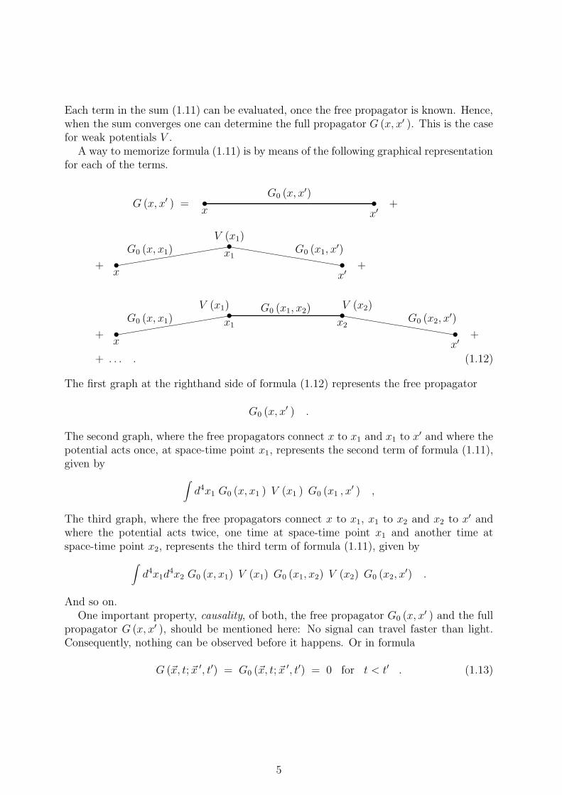
Each term in the sum (1.11) can be evaluated, once the free propagator is known. Hence,when the sum converges one can determine the full propagator G (x, x′ ). This is the casefor weak potentials V .
A way to memorize formula (1.11) is by means of the following graphical representationfor each of the terms.
G (x, x′ ) = •x
•x′
G0 (x, x′)
+
+ •x
•x′
((((((((((((G0 (x, x1)V (x1)•x1hhhhhhhhhhhh
G0 (x1, x′)
+
+ •x
•x′
((((((((((((G0 (x, x1)V (x1)•
x1
G0 (x1, x2) V (x2)•x2hhhhhhhhhhhh
G0 (x2, x′)
+
+ . . . . (1.12)
The first graph at the righthand side of formula (1.12) represents the free propagator
G0 (x, x′ ) .
The second graph, where the free propagators connect x to x1 and x1 to x′ and where the
potential acts once, at space-time point x1, represents the second term of formula (1.11),given by
∫
d4x1 G0 (x, x1 ) V (x1 ) G0 (x1 , x′ ) ,
The third graph, where the free propagators connect x to x1, x1 to x2 and x2 to x′ andwhere the potential acts twice, one time at space-time point x1 and another time atspace-time point x2, represents the third term of formula (1.11), given by
∫
d4x1d4x2 G0 (x, x1) V (x1) G0 (x1, x2) V (x2) G0 (x2, x
′) .
And so on.One important property, causality, of both, the free propagator G0 (x, x
′ ) and the fullpropagator G (x, x′ ), should be mentioned here: No signal can travel faster than light.Consequently, nothing can be observed before it happens. Or in formula
G (~x, t; ~x ′, t′) = G0 (~x, t; ~x′, t′) = 0 for t < t′ . (1.13)
5
1.1.1 Proof of formula (1.9)
Below, we will study a proof of formula (1.9).
We show that by substituting expression (1.9) into formula (1.3) one ends up with theSchrodinger equation (1.7).
The substitution results in the following relation
θ (t− t′) ψ (x) = (1.14)
= i∫
d3x′
G0 (x, x′ ) +
∫
d4x′′ G0 (x, x′′ ) V (x′′ ) G (x′′ , x′ )
ψ (x′) .
Next, we let the operator
i∂
∂t− H0 (~x )
work at both sides of equation (1.14). From the lefthand side of (1.14), also using theresult (1.5), one finds
iδ (t− t′) ψ (x) + θ (t− t′)
i∂
∂t− H0 (~x )
ψ (x) . (1.15)
Whereas, from the righthand side, also using the result (1.8), we obtain
i∫
d3x′
i∂
∂t− H0 (~x )
G0 (x, x′ ) ψ (x′) +
+ i∫
d3x′∫
d4x′′
i∂
∂t− H0 (~x )
G0 (x, x′′ ) V (x′′ ) G (x′′ , x′ ) ψ (x′) =
= i∫
d3x′ δ(4) (x− x′ ) ψ (x′) +
+ i∫
d3x′∫
d4x′′ δ(4) (x− x′′ ) V (x′′ ) G (x′′ , x′ ) ψ (x′)
In the last step of equation (1.16) we used once more equation (1.3). Combining results(1.15) and (1.16) one finds the Schrodinger equation (1.7).
6
1.2 Free Klein Gordon particles
Non-interacting particles without spin or charge are described by the Klein-Gordon equa-tion, which satisfies the wave equation
∂2
∂t2ψ(x, t) =
(
∂2
∂x2− m2
)
ψ(x, t) . (1.17)
Here we define
∂µ∂µ =∂2
∂t2− ∂2
∂x2− ∂2
∂y2− ∂2
∂z2,
in order to write the Klein-Gordon equation in the usual form
(
∂µ∂µ + m2)
ψ(x) = 0 , (1.18)
where ψ(x) stands for ψ (~x, t).Notice, that we assume here that gravitational effects can be completely ignored and
consequently that our particles move in a Minkowskian background for which we adoptedthe metric (+−−−).
As easily can be verified, a general solution to the free Klein-Gordon equation (1.18)is given by the following wave packet
ψ(x) =∫
d3k
(2π)32E
α(
~k)
e−ikx + α∗(
~k)
eikx
, (1.19)
provided that k, which stands for(
E,~k)
, satisfies the mass-shell relation
E2 =(
~k)2
+ m2 . (1.20)
7
1.3 Green’s function for free Klein-Gordon particles
The Green’s function, G0, for a free Klein-Gordon particle, which has the correct boundaryconditions, is a solution of the differential equation given by
(
∂
∂xµ∂
∂xµ+ m2
)
G0 (x, x′) = δ(4) (x− x′) . (1.21)
One may construct the correct solution by defining the Fourier transform, G0, of G0, by
G0 (x, x′) =
∫
d4p
(2π)4eipx
∫
d4p′
(2π)4eip
′x′ G0 (p, p′) .
For this Fourier transform one finds, by applying the Klein-Gordon differential equation(1.21), the relation
∫
d4p
(2π)4
(
−p2 +m2)
eipx∫
d4p′
(2π)4eip
′x′ G0 (p, p′) =
∫
d4p
(2π)4eip (x− x′) ,
which is solved by
(
−p2 +m2)
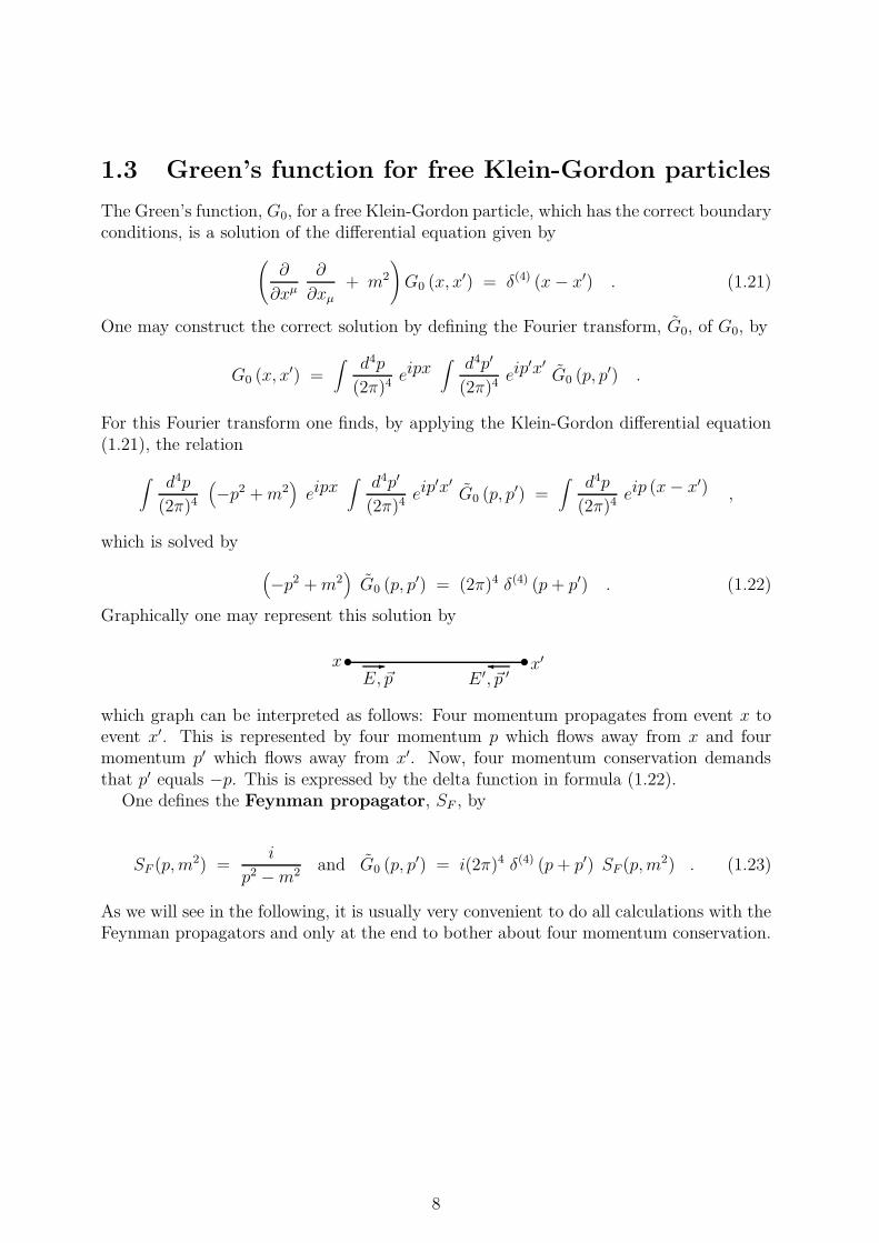
G0 (p, p′) = (2π)4 δ(4) (p+ p′) . (1.22)
Graphically one may represent this solution by
• •x -E, ~p
x′E ′, ~p ′
which graph can be interpreted as follows: Four momentum propagates from event x toevent x′. This is represented by four momentum p which flows away from x and fourmomentum p′ which flows away from x′. Now, four momentum conservation demandsthat p′ equals −p. This is expressed by the delta function in formula (1.22).
One defines the Feynman propagator, SF , by
SF (p,m2) =
i
p2 −m2 and G0 (p, p′) = i(2π)4 δ(4) (p+ p′) SF (p,m
2) . (1.23)
As we will see in the following, it is usually very convenient to do all calculations with theFeynman propagators and only at the end to bother about four momentum conservation.
8
1.4 Second Quantization Procedure
Our goal is to describe many interacting particles, not just one-particle states. To thataim we define a Hilbert space of many-particle states, also called Fock space.
The most elementary state of this space is called the vacuum, symbolized by |0〉. Itis assumed to be the state with no particles at all or just simply the ground state of thesystem of states one considers.
Next in the hierarchy come the one-particle states, for our world, just existing of Klein-Gordon particles, denoted by
∣
∣
∣
~k⟩
. It is supposed to describe a particle with momentum ~k.
The operator, which creates out of the vacuum a one-particle state, is denoted by a†(
~k)
.Consequently, we may write
∣
∣
∣
~k⟩
= a†(
~k)
|0〉 . (1.24)
Two-particle states, which describe the situation in which in our world only two parti-cles are present, one with momentum ~k1 and the other with momentum ~k2, are supposedto be given by
∣
∣
∣
~k1, ~k2⟩
= a†(
~k1)
a†(
~k2)
|0〉 . (1.25)
Now, we suppose that the order in which the particles are created, which is not a time-order but just an operation order, does not influence in any way the resulting two-particlestate. Hence, we find as a property of the creation operators defined in formula (1.24)that they commute, i.e.
a†(
~k1)
a†(
~k2)
= a†(
~k2)
a†(
~k1)
. (1.26)
We also define annihilation operators, a(
~k)
, with the following properties
a(
~k)
|0〉 = 0 ,
a(
~k1)
a(
~k2)
= a(
~k2)
a(
~k1)
, and
[
a(
~k1)
, a†(
~k2)]
= (2π)3 2E1 δ(3)(
~k1 − ~k2)
. (1.27)
Notice that the commutation relations for the creation and annihilation operators arethe continuum generalizations of the commutators for n harmonic oscillators, which alsovanish except for
[
ai , a†j
]
= δij .
The next step in the second quantization procedure is the replacement of the free Klein-Gordon wave packet, which is defined in formula (1.19), by a free Klein-Gordon quantumfield, i.e.
φ(x) =∫
d3k
(2π)32E
a(
~k)
e−ikx + a†(
~k)
eikx
, (1.28)
which is an operator which acts in the many-particle state Hilbert space.
9
The reason why this procedure is called second quantization stems from the fact thatwe can also define a conjugate momentum
π(x) =∂
∂tφ(x) , (1.29)
for which one has the following equal time commutation relations
First, we write the explicit expression for the conjugate momentum π (~x, t) of φ (~x, t),namely
π (~x, t) =∂
∂tφ (~x, t)
=∫
d3k
(2π)32EiE
− a(
~k)
ei(
~k · ~x−Et)
+ a†(
~k)
e−i(
~k · ~x− Et)
= i∫
d3k
2(2π)3
− a(
~k)
ei(
~k · ~x− Et)
+ a†(
~k)
e−i(
~k · ~x−Et)
. (1.31)
Then, we substitute formulas (1.28) for the field and (1.31) for its conjugate momentumin the expression for the equal-time commutators (1.30). This gives:
[φ (~x, t) , φ (~x ′, t)] =∫
d3k
(2π)32E
∫
d3k′
(2π)32E ′
[
a(
~k)
, a(
~k ′)]
ei(
~k · ~x+ ~k ′ · ~x ′ − (E + E ′) t)
+
+[
a(
~k)
, a†(
~k ′)]
ei(
~k · ~x− ~k ′ · ~x ′ − (E −E ′) t)
+
+[
a†(
~k)
, a(
~k ′)]
ei(
−~k · ~x+ ~k ′ · ~x ′ − (−E + E ′) t)
+
+[
a†(
~k)
, a†(
~k ′)]
ei(
−~k · ~x− ~k ′ · ~x ′ + (E + E ′) t)
Next, we insert expressions (1.26) and (1.27) to find
[φ (~x, t) , φ (~x ′, t)] =∫
d3k
(2π)32E
∫
d3k′
(2π)32E ′
10
(2π)32Eδ(3)(
~k − ~k ′)
ei(
~k · ~x− ~k ′ · ~x ′ − (E − E ′) t)
+
− (2π)32Eδ(3)(
~k − ~k ′)
ei(
−~k · ~x+ ~k ′ · ~x ′ − (−E + E ′) t)
Upon integration over ~k ′, we obtain ~k ′ = ~k and
E ′ =
√
(
~k ′)2
+m2 =
√
(
~k)2
+m2 = E
hence
[φ (~x, t) , φ (~x ′, t)] =∫
d3k
(2π)32E
ei~k · (~x− ~x ′) − e−i~k · (~x− ~x ′)
.
In the second term one may perform the substition ~k ↔ −~k for the integration variable,in order to obtain two equal terms with opposite sign and thus
[φ (~x, t) , φ (~x ′, t)] = 0 .
The proof for the equal-time commutator of two conjugate momentum fields is verysimilar.
For the equal-time commutator of the field and its conjugate momentum we obtain
[π (~x, t) , φ (~x ′, t)] =∫
id3k
2(2π)3
∫
d3k′
(2π)32E ′
−[
a(
~k)
, a†(
~k ′)]
ei(
~k · ~x− ~k ′ · ~x ′ − (E − E ′) t)
+
+[
a†(
~k)
, a(
~k ′)]
ei(
−~k · ~x+ ~k ′ · ~x ′ − (−E + E ′) t)
=∫ id3k
2(2π)3
∫ d3k′
(2π)32E ′
−(2π)32Eδ(3)(
~k − ~k ′)
ei(
~k · ~x− ~k ′ · ~x ′ − (E −E ′) t)
+
− (2π)32Eδ(3)(
~k − ~k ′)
ei(
−~k · ~x+ ~k ′ · ~x ′ − (−E + E ′) t)
=∫
id3k
2(2π)3
− ei~k · (~x− ~x ′) − e−i~k · (~x− ~x ′)
= −i∫
d3k
(2π)3ei~k · (~x− ~x ′)
= −iδ(3) (~x− ~x ′) .
11
1.5 Self-interacting Klein-Gordon field
In general, one starts a quantum field theory by defining a Lagrangian density, L, whichis a functional of a quantum field, ϕ, and its derivatives
L(
ϕ (~x, t) , ∂µ ϕ (~x, t))
. (1.32)
The object ∂µϕ in formula (1.32) stands for the four partial derivatives given by
∂0ϕ =∂
∂tϕ , ∂1ϕ =
∂
∂xϕ , ∂2ϕ =
∂
∂yϕ , and ∂3ϕ =
∂
∂zϕ .
The total Lagrangian, L, for the system under consideration is given by the volumeintegral of the Lagrangian density over all space
L =∫
d3x L(
ϕ (~x, t) , ∂µ ϕ (~x, t))
.
All dynamics of the system is contained in the Lagrangian density.The field equations for the quantum field can be derived from the Lagrangian density
by the use of the Euler-Lagrange equations
∂L∂ϕ
= ∂µ∂L
∂(
∂µϕ) , (1.33)
where
∂µ∂L
∂(
∂µϕ) = ∂0
∂L∂ (∂0ϕ)
− ∂1∂L
∂ (∂1ϕ)− ∂2
∂L∂ (∂2ϕ)
− ∂3∂L
∂ (∂3ϕ).
Now, the Lagrangian density for the self-interacting scalar field, or Klein-Gordon field,which we will consider here, is given by
L(
ϕ, ∂µ ϕ)
=1
2
(
∂µ ϕ)2 − 1
2m2ϕ2 − λ
4!ϕ4 , (1.34)
where(
∂µ ϕ)2
= (∂0 ϕ)2 − (∂1 ϕ)
2 − (∂2 ϕ)2 − (∂3 ϕ)
2 .
The theory, which follows from the above Lagrangian density (1.34), is in the literatureknown as ϕ4 theory.
Applying the Euler-Lagrange equations (1.33) to the Lagrangian density (1.34), yieldsthe following quantum field equation
(
∂µ∂µ + m2)
ϕ(x) = − λ3!ϕ3(x) . (1.35)
When we compare the field equation (1.35) to the wave equation (1.18) for a free Klein-Gordon particle we may conclude that, for vanishing λ, equation (1.35) may be interpretedas the field equation for a free Klein-Gordon field. The term on the righthand side ofequation (1.35), which stems from the term −λϕ4/4! in the Lagrangian density (1.34),
12
may be interpreted as the source term which describes the deviation of the theory for self-interacting particles from the free theory because of the presence of interaction betweenthe particles. For this reason we split the Lagrangian density in two parts, the freeLagrangian density L0 and the interaction part Lint, defined by
L0 =1
2
(
∂µ ϕ)2 − 1
2m2ϕ2 and Lint = − λ
4!ϕ4 . (1.36)
The first term in L0, which generates the term ∂µ∂µ ϕ in the field equation and istherefore related to the momentum squared of a free Klein-Gordon particle, is called thekinetic term; the second term in L0 the mass term.
As been observed above, in the absence of the source term the field equation (1.35)describes a free scalar quantum field, φ, for which the expression (1.28) is a generalsolution.
As mentioned before, the objects of our interest are the n-point Green’s functions,which we are now capable of defining
G (x1, . . . , xn) =
⟨
0∣
∣
∣
∣
T
φ (x1) · · ·φ (xn) ei∫
d4y Lint (φ(y))∣
∣
∣
∣
0⟩
⟨
0
∣
∣
∣
∣
T
ei∫
d4y Lint (φ(y))∣
∣
∣
∣
0⟩ , (1.37)
where T stands for time-ordering, which means that in all expressions the fields must bepermuted in such a way that the time components of their arguments are decreasing.
13
1.6 Time-ordered product of two fields
In this section we determine in all detail the vacuum expectation value of the time orderedproduct of two boson fields, also called propagator, and which is defined by
〈0 |T φ (x1)φ (x2)| 0〉 . (1.38)
When we express the time-ordering in terms of the θ-function, defined in (1.2), whichvanishes for negative argument and equals 1 for positive argument, then we obtain thefollowing two terms
The full expressions for those objects, after the substitution of formula (1.28) for the fields,are also quite long, but things become more managable by the use of the definitions
a(x) =∫ d3k
(2π)32Ee−ikx a
(
~k)
and φ(x) = a(x) + a†(x) . (1.41)
Substituting those definitions into the first term of formula (1.40), one obtains for thevacuum expectation value of two fields
⟨
0∣
∣
∣
a (x1) + a† (x1)
a (x2) + a† (x2)∣
∣
∣ 0⟩
, (1.42)
which upon multiplication leaves us with the following four terms
〈0 |a (x1) a (x2)| 0〉 +⟨
0∣
∣
∣a† (x1) a (x2)∣
∣
∣ 0⟩
+⟨
0∣
∣
∣a (x1) a† (x2)
∣
∣
∣ 0⟩
+⟨
0∣
∣
∣a† (x1) a† (x2)
∣
∣
∣ 0⟩
.
(1.43)Three of the four terms in the expansion (1.43) vanish, as for example one has from thedefinition (1.27) for the annihilation operators that
a(x)|0〉 =∫
d3k
(2π)32Ee−ikx a
(
~k)
|0〉 = 0 , (1.44)
and hence, for a creation operator
〈0|a†(x) = a(x)|0〉† = 0 . (1.45)
As a consequence of those properties for the operators defined in formula (1.41), we arethen left with only one nonzero contribution to first of the two vacuum expectation values(1.40) of two fields, i.e.
〈0 |φ (x1)φ (x2)| 0〉 =⟨
0∣
∣
∣a (x1) a† (x2)
∣
∣
∣ 0⟩
, (1.46)
14
which, upon insertion of the full expression (1.41) for the operators a(x) and a†(x), reads
∫
d3k1(2π)32E1
∫
d3k2(2π)32E2
e−ik1x1 + ik2x2⟨
0∣
∣
∣a(
~k1)
a†(
~k2)∣
∣
∣ 0⟩
and hence contains the vacuum expectation value
⟨
0∣
∣
∣a(
~k1)
a†(
~k2)∣
∣
∣ 0⟩
.
The latter expression can easily be handled by the use of the commutation relations (1.27)and the properties (1.27) for the annihilation operators, which leads to
⟨
0∣
∣
∣a(
~k1)
a†(
~k2)∣
∣
∣ 0⟩
=⟨
0∣
∣
∣
[
a(
~k1)
, a†(
~k2)]
+ a†(
~k2)
a(
~k1)∣
∣
∣ 0⟩
= 〈0 |0〉(2π)32E1δ(3)(
~k1 − ~k2)
+⟨
0∣
∣
∣a†(
~k2)
a(
~k1)∣
∣
∣ 0⟩
= (2π)32E1δ(3)(
~k1 − ~k2)
,
and which turns expression (1.46) into
〈0 |φ (x1)φ (x2)| 0〉 =∫
d3k1(2π)32E1
∫
d3k2(2π)32E2
e−ik1x1 + ik2x2 (2π)32E1δ(3)(
~k1 − ~k2)
.
Because of the Dirac delta function, one may perform the ~k2-integration and then renamethe dummy ~k1 integration variable for ~k. This gives the vacuum expectation value offormula (1.46) its final form
〈0 |φ (x1)φ (x2)| 0〉 =∫ d3k
(2π)32Ee−ik (x1 − x2) (1.47)
The second term of formula (1.40) equals the first term with the numbers one and twoexchanged. So, we obtain for the vacuum expectation value (1.39) of the time orderedproduct of two boson fields the expression
〈0 |T φ (x1)φ (x2)| 0〉 =
∫ d3k(2π)32E
e−ik (x1 − x2) for t1〉t2∫ d3k(2π)32E
e−ik (x2 − x1) for t1〈t2. (1.48)
Now, in the exponents of (1.48) comes kx, which in our metric equals Et− ~k · ~x. Hence,in the above expression we must take E (t1 − t2) for t1〉t2 and E (t2 − t1) for t1〈t2, whichis equivalent to taking E |t1 − t2| irrespective of the order of t1 and t2, i.e.
〈0 |T φ (x1)φ (x2)| 0〉 =
∫ d3k(2π)32E
ei~k · (~x1 − ~x2)− iE |t1 − t2| for t1〉t2
∫ d3k(2π)32E
ei~k · (~x2 − ~x1)− iE |t1 − t2| for t1〈t2
.
(1.49)
15
Furthermore, by changing the integration variable ~k to −~k in the lower of the two expres-sions in formula (1.49), results
〈0 |T φ (x1)φ (x2)| 0〉 =∫
d3k
(2π)32Eei~k · (~x1 − ~x2)− iE |t1 − t2| . (1.50)
With complex function theory one can easily show the following identity
i∫ +∞
−∞
dk02π
e−ik0t
(k0)2 −
(
~k)2 −m2
=e−i√
(
~k)2
+m2 |t|
2
√
(
~k)2
+m2
, (1.51)
which, upon substitution in formula (1.50),
also remembering that E actually stands for
√
(
~k)2
+m2, gives
〈0 |T φ (x1)φ (x2)| 0〉 = i∫
d4k
(2π)4e−ik (x1 − x2)
k2 −m2 , (1.52)
where k stands for(
k0, ~k)
and d4k for dk0d3k.
Notice, that, since k0 is an integration variable, k2, which equals (k0)2 −
(
~k)2, is not
identical to m2, i.e. is off-mass-shell.
A graphical representation for the propagator (1.52) is as shown below.
• •x1 x2k
One might moreover recognize in the final expression (1.52) for the vacuum expectationvalue of the time ordered product of two boson fields the Feynman propagator which isgiven in formula (1.23).
1.6.1 Proof of formula (1.51)
For the proof of formula (1.51), which we cast here in the form
i∫ +∞
−∞
dk02π
e−ik0t(k0)
2 −M2=
e−iM |t|2M
, (1.53)
we introduce a small positive real number ǫ, such that the righthand side of equation(1.53) gives
e−iM |t| − ǫ |t|2M +O(ǫ) , (1.54)
which vanishes in the limits t→ ±∞.At the end of the calculations we take ǫ ↓ 0.By comparison of formulae (1.53) and (1.54), we conclude that we must choose the
substitutionM −→ M − iǫ . (1.55)
16
The integral which consequently has to be calculated is then
i∫ +∞
−∞
dk02π
e−ik0t(k0 −M + iǫ) (k0 +M − iǫ) . (1.56)
In the literature one often finds the form
i∫ +∞
−∞
dk02π
e−ik0t(k0)
2 −M2 + iǫ. (1.57)
This can be achieved from expression (1.56) by the substitution
2Mǫ −→ ǫ , (1.58)
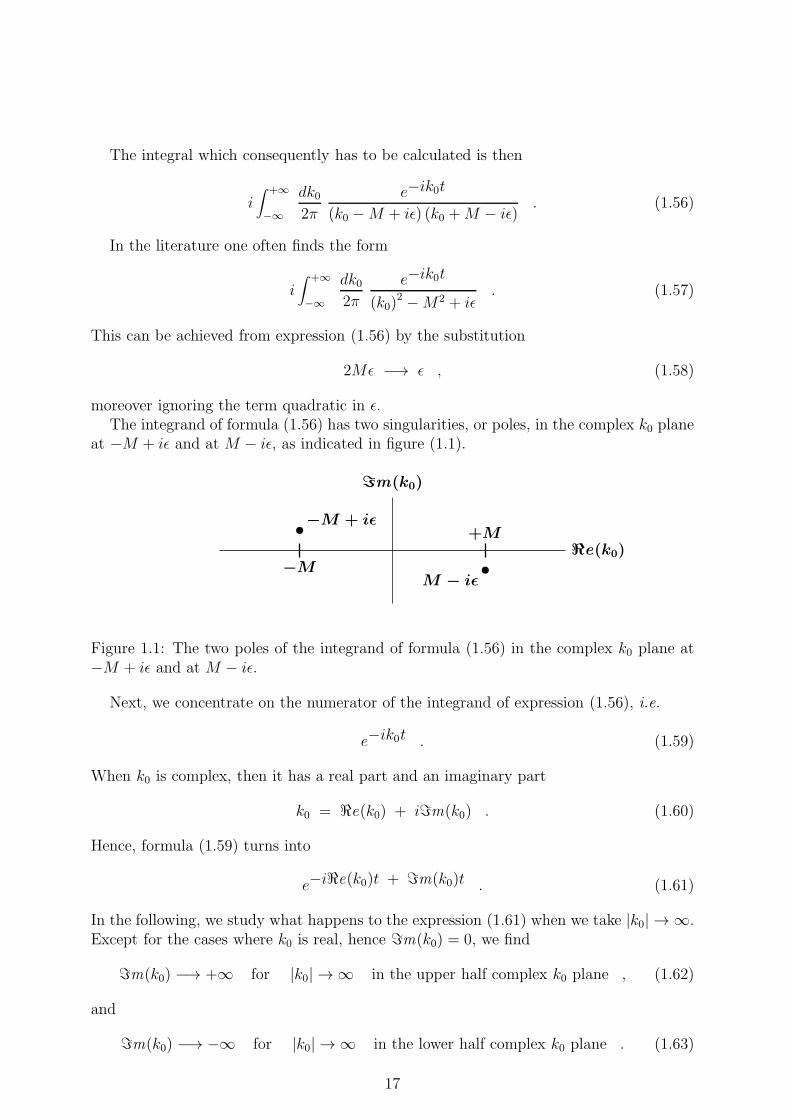
moreover ignoring the term quadratic in ǫ.The integrand of formula (1.56) has two singularities, or poles, in the complex k0 plane
at −M + iǫ and at M − iǫ, as indicated in figure (1.1).
•−M + iǫ
−M
+M
•M − iǫ
ℜe(k0)
ℑm(k0)
Figure 1.1: The two poles of the integrand of formula (1.56) in the complex k0 plane at−M + iǫ and at M − iǫ.
Next, we concentrate on the numerator of the integrand of expression (1.56), i.e.
e−ik0t . (1.59)
When k0 is complex, then it has a real part and an imaginary part
k0 = ℜe(k0) + iℑm(k0) . (1.60)
Hence, formula (1.59) turns into
e−iℜe(k0)t + ℑm(k0)t . (1.61)
In the following, we study what happens to the expression (1.61) when we take |k0| → ∞.Except for the cases where k0 is real, hence ℑm(k0) = 0, we find
ℑm(k0) −→ +∞ for |k0| → ∞ in the upper half complex k0 plane , (1.62)
and
ℑm(k0) −→ −∞ for |k0| → ∞ in the lower half complex k0 plane . (1.63)
17
Consequently, for t < 0, we obtain
e−iℜe(k0)t + ℑm(k0)t −→ 0 for |k0| → ∞ in the upper half complex k0 plane ,(1.64)
whereas, for t > 0, we obtain
e−iℜe(k0)t + ℑm(k0)t −→ 0 for |k0| → ∞ in the lower half complex k0 plane ,(1.65)
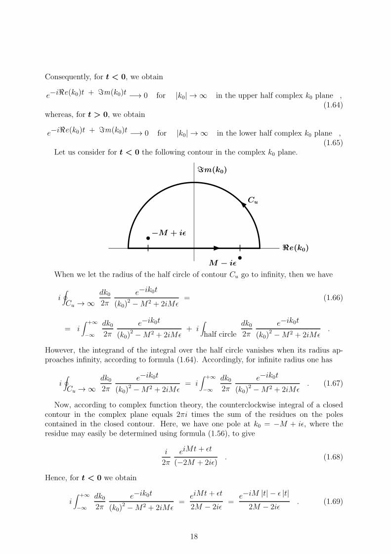
Let us consider for t < 0 the following contour in the complex k0 plane.
•−M + iǫ
•M − iǫ
ℜe(k0)
ℑm(k0)
Cu
When we let the radius of the half circle of contour Cu go to infinity, then we have
i∮
Cu →∞dk02π
e−ik0t(k0)
2 −M2 + 2iMǫ= (1.66)
= i∫ +∞
−∞
dk02π
e−ik0t(k0)
2 −M2 + 2iMǫ+ i
∫
half circle
dk02π
e−ik0t(k0)
2 −M2 + 2iMǫ.
However, the integrand of the integral over the half circle vanishes when its radius ap-proaches infinity, according to formula (1.64). Accordingly, for infinite radius one has
i∮
Cu →∞dk02π
e−ik0t(k0)
2 −M2 + 2iMǫ= i
∫ +∞
−∞
dk02π
e−ik0t(k0)
2 −M2 + 2iMǫ. (1.67)
Now, according to complex function theory, the counterclockwise integral of a closedcontour in the complex plane equals 2πi times the sum of the residues on the polescontained in the closed contour. Here, we have one pole at k0 = −M + iǫ, where theresidue may easily be determined using formula (1.56), to give
i
2π
eiMt + ǫt
(−2M + 2iǫ). (1.68)
Hence, for t < 0 we obtain
i∫ +∞
−∞
dk02π
e−ik0t(k0)
2 −M2 + 2iMǫ=
eiMt + ǫt
2M − 2iǫ=
e−iM |t| − ǫ |t|2M − 2iǫ
. (1.69)
18
For t > 0 we consider the following contour in the complex k0 plane.
•−M + iǫ
•M − iǫ
ℜe(k0)
ℑm(k0)
Cℓ
The integrand of the integral over the half circle vanishes when its radius approachesinfinity, according to formula (1.65). Accordingly, for infinite radius one has here
i∮
Cℓ →∞dk02π
e−ik0t(k0)
2 −M2 + 2iMǫ= i
∫ +∞
−∞
dk02π
e−ik0t(k0)
2 −M2 + 2iMǫ. (1.70)
Furthermore, according to complex function theory, the clockwise integral of a closedcontour in the complex plane equals −2πi times the sum of the residues on the polescontained in the closed contour. Here, we have one pole at k0 =M− iǫ, where the residuemay easily be determined using formula (1.56), to give
i
2π
e−iMt − ǫt(2M − 2iǫ)
. (1.71)
Hence, for t > 0 we obtain
i∫ +∞
−∞
dk02π
e−ik0t(k0)
2 −M2 + 2iMǫ=
e−iMt − ǫt2M − 2iǫ
=e−iM |t| − ǫ |t|
2M − 2iǫ. (1.72)
By comparison of formulae (1.69) and (1.72), we find for any sign of t the result
i∫ +∞
−∞
dk02π
e−ik0t(k0)
2 −M2 + 2iMǫ=
e−iM |t| − ǫ |t|2M − 2iǫ
. (1.73)
Taking the limit ǫ ↓ 0, one finds formula (1.53).
19
1.7 Time-ordered product of four fields
In this section we determine in all detail the vacuum expectation value of the time orderedproduct of four boson fields, which is defined by
〈0 |T φ (x1)φ (x2)φ (x3)φ (x4)| 0〉 . (1.74)
When we express the time-ordering in terms of the θ-function, then we obtain the followingtwenty-four terms
i.e. each term being characterized by one of the twenty-four permutations of the numbersone to four.
From expression (1.75) we learn that the first thing to be calculated, is the simplevacuum expectation value of four fields. There are twenty-four of them, which are all justpermutations of the first, given by
〈0 |φ (x1)φ (x2)φ (x3)φ (x4)| 0〉 . (1.76)
The full expression for this object is also quite long, but things become more managableby the use of the definitions given in formula (1.41). Substituting those definitions intothe expression of formula (1.76) for the simple vacuum expectation value of four fields,one obtains
⟨
0∣
∣
∣
a (x1) + a† (x1)
a (x2) + a† (x2)
a (x3) + a† (x3)
a (x4) + a† (x4)∣
∣
∣ 0⟩
. (1.77)
Here we perform the various multiplications, to end up with sixteen terms given by
〈0 |a (x1) a (x2) a (x3) a (x4)| 0〉 +⟨
0∣
∣
∣a† (x1) a (x2) a (x3) a (x4)∣
∣
∣ 0⟩
+
+⟨
0∣
∣
∣a (x1) a† (x2) a (x3) a (x4)
∣
∣
∣ 0⟩
+ · · · . (1.78)
Several of the terms in the expansion (1.78) vanish because of the properties (1.44) and(1.45) for the operators defined in formula (1.41).
More complicated cases, like
⟨
0∣
∣
∣a (x1) a (x2) a (x3) a† (x4)
∣
∣
∣ 0⟩
,
which, according to the definitions (1.41), equals
20
∫
d3k1(2π)32E1
∫
d3k2(2π)32E2
∫
d3k3(2π)32E3
∫
d3k4(2π)32E4
×
× e−ik1x1 − ik2x2 − ik3x3 + ik4x4⟨
0∣
∣
∣a(
~k1)
a(
~k2)
a(
~k3)
a†(
~k4)∣
∣
∣ 0⟩
(1.79)
and hence contains the vacuum expectation value
⟨
0∣
∣
∣a(
~k1)
a(
~k2)
a(
~k3)
a†(
~k4)∣
∣
∣ 0⟩
,
can be handled by the use of the commutation relations (1.27), which leads to
⟨
0∣
∣
∣a(
~k1)
a(
~k2)
a(
~k3)
a†(
~k4)∣
∣
∣ 0⟩
=
=⟨
0∣
∣
∣a(
~k1)
a(
~k2) [
a(
~k3)
, a†(
~k4)]
+ a†(
~k4)
a(
~k3)∣
∣
∣ 0⟩
=⟨
0∣
∣
∣a(
~k1)
a(
~k2)∣
∣
∣ 0⟩
(2π)32E3δ(3)(
~k3 − ~k4)
+⟨
0∣
∣
∣a(
~k1)
a(
~k2)
a†(
~k4)
a(
~k3)∣
∣
∣ 0⟩
= 0 .
Inspection of all sixteen terms of (1.78) gives as a result that fourteen of those vanish.We are then left with only two nonzero contributions
〈0 |φ (x1)φ (x2)φ (x3)φ (x4)| 0〉 = (1.80)
=⟨
0∣
∣
∣a (x1) a (x2) a† (x3) a
† (x4)∣
∣
∣ 0⟩
+⟨
0∣
∣
∣a (x1) a† (x2) a (x3) a
† (x4)∣
∣
∣ 0⟩
.
This can easily be seen, since, first, a vacuum expectation value for an operator whichdoes not have an equal number of creation and annihilation operators, like the one givenin formula (1.79), allways ends up with an annihilation operator acting on |0〉 or a creationoperator acting on 〈0|, by the use of commutation relations (1.27) whenever necessary.Moreover, a vacuum expectation value also vanishes when a creation operator standson the lefthand side or when an annihilation operator stands on the righthand side.Consequently, for x1 we must have an annihilation operator and for x4 a creation operator.This then implies that for x2 and x3 we must have one annihilation and one creationoperator. There are only two possibilities, which are shown in formula (1.80).
The first term of (1.80), which, in a way similar to formula (1.79), contains the vacuumexpectation value
⟨
0∣
∣
∣a(
~k1)
a(
~k2)
a†(
~k3)
a†(
~k4)∣
∣
∣ 0⟩
,
can be handled by the use of the commutation relations (1.27). First, we commute a(
~k2)
and a†(
~k3)
, which leads to
⟨
0∣
∣
∣a(
~k1)
a†(
~k4)∣
∣
∣ 0⟩
(2π)32E2δ(3)(
~k2 − ~k3)
+⟨
0∣
∣
∣a(
~k1)
a†(
~k3)
a(
~k2)
a†(
~k4)∣
∣
∣ 0⟩
.
21
Then, we commute in the first of the above two terms a(
~k1)
and a†(
~k4)
, whereas in the
second of the above two terms we commute as well a(
~k1)
with a†(
~k3)
, as a(
~k2)
with
a†(
~k4)
. The result of those operations is given by
4(2π)6E1E2δ(3)(
~k1 − ~k4)
δ(3)(
~k2 − ~k3)
+ 4(2π)6E1E2δ(3)(
~k1 − ~k3)
δ(3)(
~k2 − ~k4)
.
(1.81)In the second term of (1.80), which, in a way similar to formula (1.79), contains the
vacuum expectation value
⟨
0∣
∣
∣a(
~k1)
a†(
~k2)
a(
~k3)
a†(
~k4)∣
∣
∣ 0⟩
,
we commute as well a(
~k1)
with a†(
~k2)
, as a(
~k3)
with a†(
~k4)
. The result of thoseoperations is given by
4(2π)6E1E3δ(3)(
~k1 − ~k2)
δ(3)(
~k3 − ~k4)
. (1.82)
When we sum the two expressions (1.81) and (1.82) and also include the integrationsand the corresponding exponentials, we find for the vacuum expectation value of formula(1.80) the result
〈0 |φ (x1)φ (x2)φ (x3)φ (x4)| 0〉 =
=∫
d3k1(2π)32E1
∫
d3k2(2π)32E2
∫
d3k3(2π)32E3
∫
d3k4(2π)32E4
×
×
e−ik1x1 − ik2x2 + ik3x3 + ik4x4[
4(2π)6E1E2δ(3)(
~k1 − ~k4)
δ(3)(
~k2 − ~k3)
+
+4(2π)6E1E2δ(3)(
~k1 − ~k3)
δ(3)(
~k2 − ~k4)]
+
+ e−ik1x1 + ik2x2 − ik3x3 + ik4x4 4(2π)6E1E3δ(3)(
~k1 − ~k2)
δ(3)(
~k3 − ~k4)
.
Because of the Dirac delta functions, one may perform two of the four ~k-integrationsin each of the three above terms. In the first two terms we perform the ~k3 and the ~k4integrations. In the third term we perform the ~k2 and the ~k4 integrations, and then renamethe ~k3 integration variable for ~k2. This gives the vacuum expectation value of formula(1.80) its final form
Not a very terrible result, but remember that the vacuum expectation value (1.75) of thetime ordered product of four boson fields contains twenty-four of such terms, which nowhas to be multiplied by three. So, we have ended up with seventy-two terms, hence somebookkeeping is in order.
For convenience we define
A (x1 − x2) =∫
d3k
(2π)32Ee−ik (x1 − x2) . (1.84)
Using this definition and the result (1.83), we obtain for the vacuum expectation value(1.75) of the time ordered product of four boson fields the expression
〈0 |T φ (x1)φ (x2)φ (x3)φ (x4)| 0〉 =
= A (x1 − x4)A (x2 − x3) + A (x1 − x3)A (x2 − x4) +
+ (all possible permutations of 1,2,3 and 4) . (1.85)
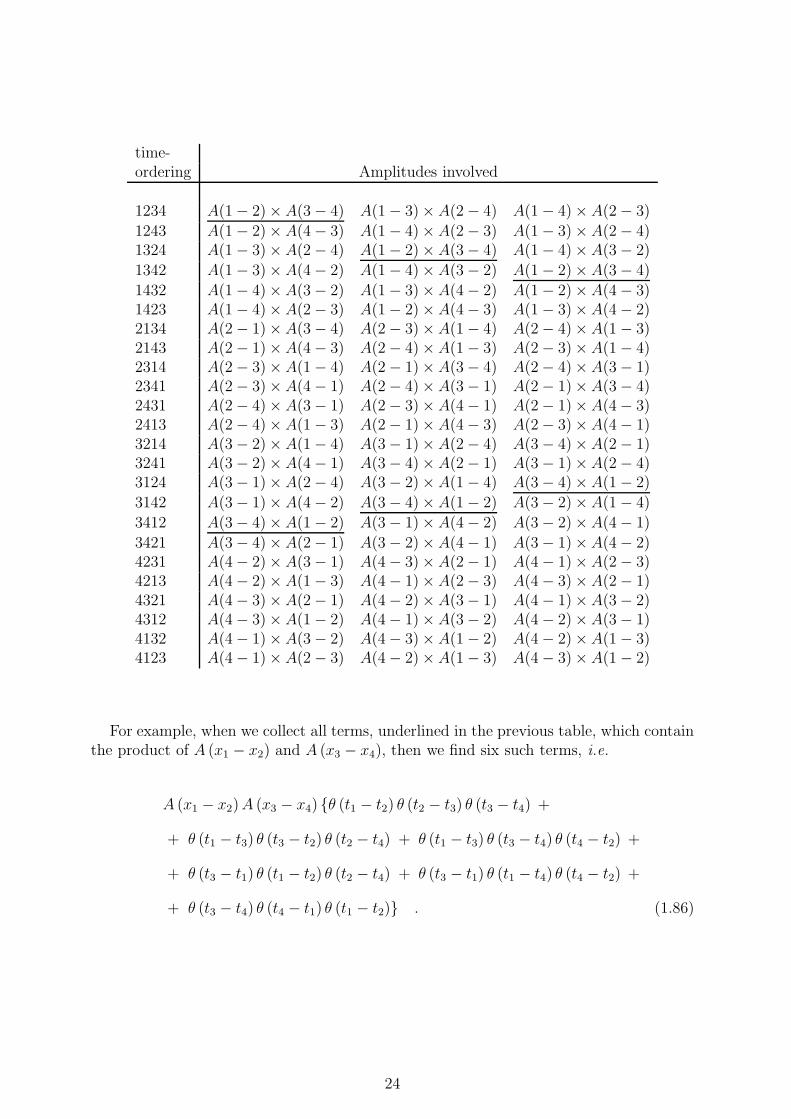
Indeed 24× 3 = 72 terms! However, as we will see in the following, their number can bereduced to three. By inspection of all twenty-four permutations of (1.85), we find thatthere are several terms which contain the same combination of A’s. Notice, from theirdefinition (1.84), that the order of the A’s in a product of A’s does not matter, but thatthe order of the coordinate variables x inside one A do matter. In the following table,where we denote t1〉t2〉t3〉t4 by 1234 and similar for the other time-orderings, we havecollected all twenty-four possible time-orderings which contribute to (1.85) and the A’sto which they are multiplied.
For example, when we collect all terms, underlined in the previous table, which containthe product of A (x1 − x2) and A (x3 − x4), then we find six such terms, i.e.
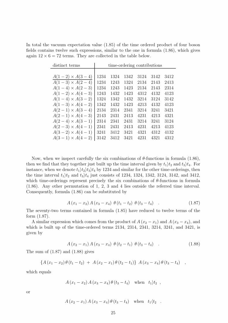
In total the vacuum expectation value (1.85) of the time ordered product of four bosonfields contains twelve such expressions, similar to the one in formula (1.86), which givesagain 12× 6 = 72 terms. They are collected in the table below.
Now, when we inspect carefully the six combinations of θ-functions in formula (1.86),then we find that they together just built up the time interval given by t1〉t2 and t3〉t4. Forinstance, when we denote t1〉t2〉t3〉t4 by 1234 and similar for the other time-orderings, thenthe time interval t1〉t2 and t3〉t4 just consists of 1234, 1324, 1342, 3124, 3142, and 3412,which time-orderings represent precisely the six combinations of θ-functions in formula(1.86). Any other permutation of 1, 2, 3 and 4 lies outside the referred time interval.Consequently, formula (1.86) can be substituted by
The seventy-two terms contained in formula (1.85) have reduced to twelve terms of theform (1.87).
A similar expression which comes from the product of A (x2 − x1) and A (x3 − x4), andwhich is built up of the time-ordered terms 2134, 2314, 2341, 3214, 3241, and 3421, isgiven by
Continuing the above procedure, all seventy-two terms of (1.85) can be summed setwisein six sets of twelve terms. For example, another such set of twelve terms sums up to
i∫
d4k
(2π)4e−ik (x1 − x2)
k2 −m2 A (x4 − x3) θ (t4 − t3) . (1.90)
Now, at this stage, it might be clear that, along the same reasoning which lead to formula(1.89), we obtain for the sum of (1.89) and (1.90) the result
i2∫
d4k1(2π)4
e−ik1 (x1 − x2)(k1)
2 −m2
∫
d4k2(2π)4
e−ik2 (x3 − x4)(k2)
2 −m2. (1.91)
A set of twenty-four terms of (1.85) neatly summed up in a compact expression. Theother two sets of twenty-four terms yield:
i2∫ d4k1
(2π)4e−ik1 (x1 − x3)
(k1)2 −m2
∫ d4k2(2π)4
e−ik2 (x2 − x4)(k2)
2 −m2, (1.92)
and
i2∫
d4k1(2π)4
e−ik1 (x1 − x4)(k1)
2 −m2
∫
d4k2(2π)4
e−ik2 (x2 − x3)(k2)
2 −m2. (1.93)
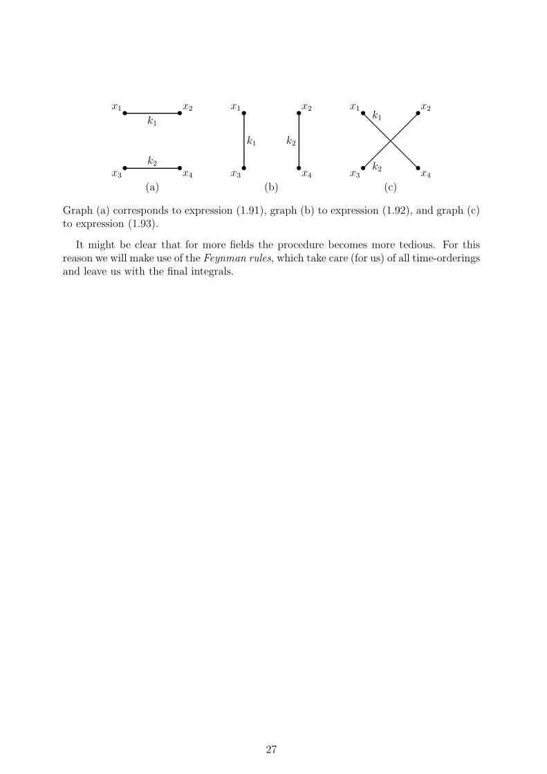
The whole vacuum expectation value of the time ordered product of four boson fieldsis just given by the sum of the three expressions, (1.91), (1.92), and (1.93). Each of thoseexpressions is just the product of two Feynman propagators as given in formula (1.52).
A graphical representation for the three expressions, (1.91), (1.92), and (1.93), can beconstructed as follows: The coordinates x1, x2, x3, and x4 are represented by four dots,as shown below.
•
•
•
•
x3
x1
x4
x2
Each possible pairwise connection of those dots represents one of the three above expres-sions according to the combination of coordinates in the exponents. The three possiblepairwise connections are given below.
26
•
•
•
•
x3
x1
x4
x2
k2
k1
(a)
•
•
•
•
x3
x1
x4
x2
k2k1
(b)
•
•
•
•
x3
x1
x4
x2
@
@@
@@@k2
k1
(c)
Graph (a) corresponds to expression (1.91), graph (b) to expression (1.92), and graph (c)to expression (1.93).
It might be clear that for more fields the procedure becomes more tedious. For thisreason we will make use of the Feynman rules, which take care (for us) of all time-orderingsand leave us with the final integrals.
27
1.8 Feynman rules (part I)
In order to determine an analytic expression for the vacuum expection value of a time-ordered product of n fields, given by
〈0 |T φ (x1) · · ·φ (xn)| 0〉 , (1.94)
one proceeds as follows. Each field φ in ( 1.94) brings, following the definition ( 1.28) forthe quantum fields as well as the procedure which lead from formula ( 1.48) to formula( 1.52), a Fourier transform integration of the form
∫
d4ki(2π)4
e−ikixi for i = 1, . . . , n . (1.95)
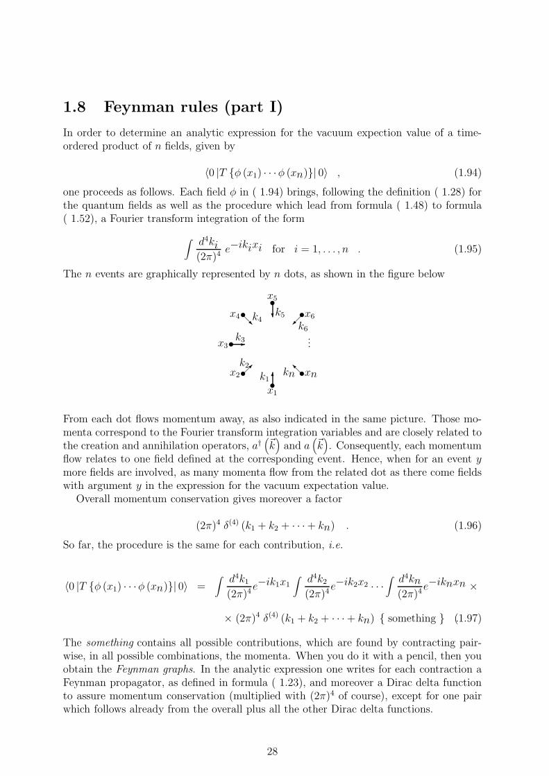
The n events are graphically represented by n dots, as shown in the figure below
•x16k1•x2
k2
•x3 -k3
•x4@Rk4
•x5?k5 •x6
k6...
•xn@Ikn
From each dot flows momentum away, as also indicated in the same picture. Those mo-menta correspond to the Fourier transform integration variables and are closely related tothe creation and annihilation operators, a†
(
~k)
and a(
~k)
. Consequently, each momentumflow relates to one field defined at the corresponding event. Hence, when for an event ymore fields are involved, as many momenta flow from the related dot as there come fieldswith argument y in the expression for the vacuum expectation value.
Overall momentum conservation gives moreover a factor
(2π)4 δ(4) (k1 + k2 + · · ·+ kn) . (1.96)
So far, the procedure is the same for each contribution, i.e.
The something contains all possible contributions, which are found by contracting pair-wise, in all possible combinations, the momenta. When you do it with a pencil, then youobtain the Feynman graphs. In the analytic expression one writes for each contraction aFeynman propagator, as defined in formula ( 1.23), and moreover a Dirac delta functionto assure momentum conservation (multiplied with (2π)4 of course), except for one pairwhich follows already from the overall plus all the other Dirac delta functions.
28
We give below three examples, the already known vacuum expectation values of thetime-ordered products of two and four fields and a new vacuum expectation value whichalso involves some combinatorics.
I The vacuum expectation value of the time-ordered product oftwo fields.
From expression ( 1.38), following the above outlined procedure, we find for the vac-uum expectation value of the time-ordered product of two fields the following graphicrepresentation
•x1 -k1
•x2k2
Consequently, one has only one possible contraction, which leads to the analytic expressiongiven by
∫
d4k1(2π)4
e−ik1x1∫
d4k2(2π)4
e−ik2x2 (2π)4 δ(4) (k1 + k2)i
(k1)2 −m2
, (1.98)
for which it is a simple task (just perform the k2-integration) to convince oneself that thisequals the previous expression ( 1.52).
II The vacuum expectation value of the time-ordered product offour fields.
From expression ( 1.74), following the above outlined procedure, we find for the vac-uum expectation value of the time-ordered product of four fields the following graphicrepresentation
•x1@R k1
•x2k2
•x3
k3
•x4@Ik4
Consequently, the general form of the analytic expression reads
There are three different possible ways to contract the four momenta in this case, as wealready know from section ( 1.6).
29
Contracting k1 with k2 and k3 with k4 gives
(2π)4 δ(4) (k1 + k2)i
(k1)2 −m2
× i
(k3)2 −m2
.
Notice that only one of the two contractions involves a Dirac delta function for the mo-mentum conservation, the other pair is then automatically conserved because of the Diracdelta function in formule ( 1.99) for the overall momentum conservation.
The other two contributions to ( 1.99), with comparable expressions to the one above,come from the other two possible ways to contract the momenta. In total, we find then
〈0 |T φ (x1)φ (x2)φ (x3)φ (x4)| 0〉 = (1.100)
∫
d4k1(2π)4
e−ik1x1∫
d4k2(2π)4
e−ik2x2∫
d4k3(2π)4
e−ik3x3∫
d4k4(2π)4
e−ik4x4 ×
× (2π)4 δ(4) (k1 + k2 + k3 + k4) ×
×
(2π)4 δ(4) (k1 + k2)i
(k1)2 −m2
× i
(k3)2 −m2
+
+ (2π)4 δ(4) (k1 + k3)i
(k1)2 −m2
× i
(k2)2 −m2
+
+ (2π)4 δ(4) (k1 + k4)i
(k1)2 −m2
× i
(k3)2 −m2
.
After performing two of the four k-integrations one obtains the same result as given bythe sum of the three expressions, ( 1.91), ( 1.92), and ( 1.93).
30
III The vacuum expectation value of the time-ordered product ofsix fields, out of which four are at the same event.
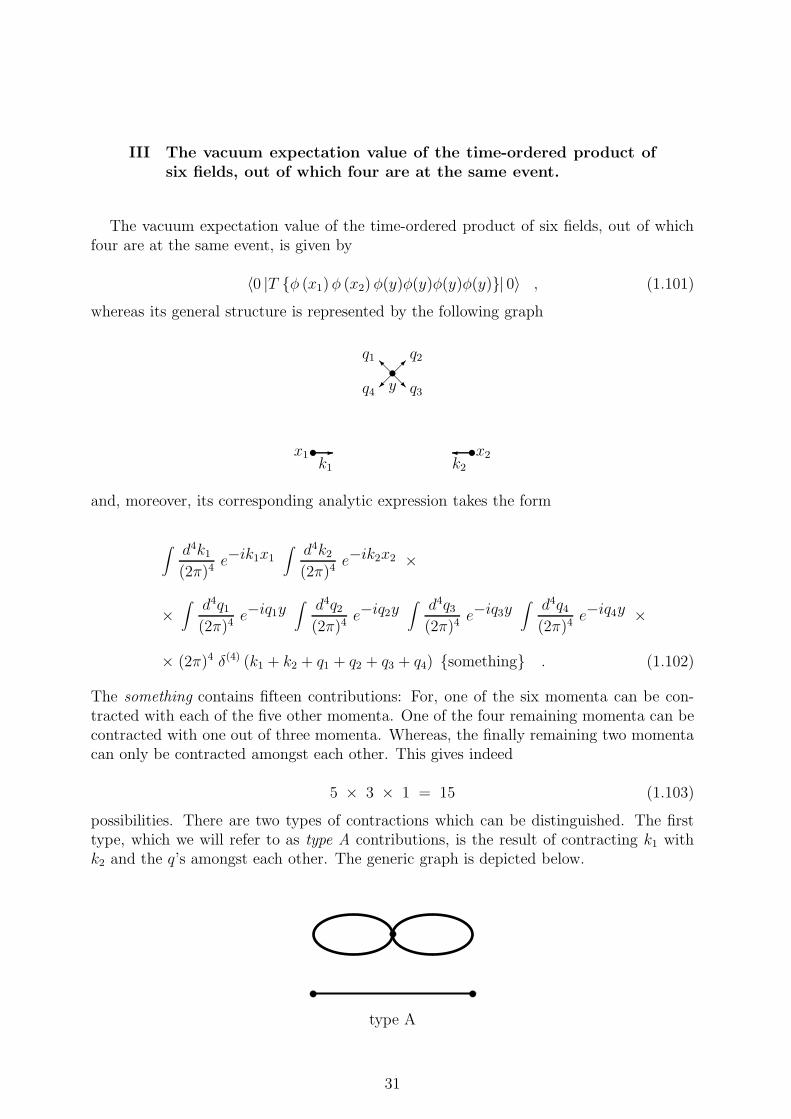
The vacuum expectation value of the time-ordered product of six fields, out of whichfour are at the same event, is given by
〈0 |T φ (x1)φ (x2)φ(y)φ(y)φ(y)φ(y)| 0〉 , (1.101)
whereas its general structure is represented by the following graph
•x1 -k1
•x2k2
•y
@Iq1
q2
@R q3q4
and, moreover, its corresponding analytic expression takes the form
The something contains fifteen contributions: For, one of the six momenta can be con-tracted with each of the five other momenta. One of the four remaining momenta can becontracted with one out of three momenta. Whereas, the finally remaining two momentacan only be contracted amongst each other. This gives indeed
5 × 3 × 1 = 15 (1.103)
possibilities. There are two types of contractions which can be distinguished. The firsttype, which we will refer to as type A contributions, is the result of contracting k1 withk2 and the q’s amongst each other. The generic graph is depicted below.
type A
31
There are three such contributions, which result all three in the same analytic expression,because one of the q’s can be contracted with each of the remaining three q’s and moreoverintegration variables are dummy. We obtain then for type A the expression
3 (2π)4 δ(4) (q1 + q4)i
(q1)2 −m2
× (2π)4 δ(4) (q2 + q3)i
(q2)2 −m2
× i
(k1)2 −m2
.
So, the type A contractions lead to the contribution
3∫
d4k1(2π)4
e−ik1x1∫
d4k2(2π)4
e−ik2x2 × (1.104)
×∫ d4q1
(2π)4e−iq1y
∫ d4q2(2π)4
e−iq2y∫ d4q3
(2π)4e−iq3y
∫ d4q4(2π)4
e−iq4y ×
× (2π)4 δ(4) (k1 + k2 + q1 + q2 + q3 + q4) ×
× (2π)4 δ(4) (q1 + q4)i
(q1)2 −m2
× (2π)4 δ(4) (q2 + q3)i
(q2)2 −m2
× i
(k1)2 −m2
.
When we perform the q3 and q4 integrations, then, because of the Dirac delta functions,we end up with
3∫ d4k1
(2π)4e−ik1x1
∫ d4k2(2π)4
e−ik2x2 (2π)4 δ(4) (k1 + k2)i
(k1)2 −m2
×
×∫
d4q1(2π)4
i
(q1)2 −m2
×∫
d4q2(2π)4
i
(q2)2 −m2
. (1.105)
The latter two integrals are so-called loop integrations since each can be associated withone of the two loops in the graph for the type A contributions. When in formula ( 1.100)one substitutes x1, x2, x3, and x4, by y one obtains exactly three times the product ofthose loop integrations. Moreover, by comparison to formula ( 1.98), one finds that thefirst part of the above expression ( 1.105) equals the vacuum expectation value of the time-ordered product of two fields. Consequently, one may write for the type A contributionsthe following identity
〈0 |T φ (x1)φ (x2)φ(y)φ(y)φ(y)φ(y)| 0〉 (type A contributions) =
Contributions, which are represented by graphs similar to the graph for the type Acontribution, i.e. graphs which have disconnected parts, are called vacuum bubbles. Theydo not play any role in real physics as we will see furtheron.
32
The second type of contributions to the something of formula ( 1.102), which we willrefer to as type B contributions, stem from the contractions of k1 and k2 each with one ofthe q’s. The generic graph is depicted below
In the literature this graph is usually drawn as shown hereafter
type B
There are twelve such contributions, which result all twelve in the same analytic expres-sion, because one of the k’s can be contracted with each of the four q’s, the other k withany of the three remaining q’s and moreover integration variables are dummy, which gives
4 × 3 = 12 (1.107)
contributions. We obtain then for type B the expression
12 (2π)4 δ(4) (k1 + q1)i
(k1)2 −m2
× (2π)4 δ(4) (k2 + q2)i
(k2)2 −m2
× i
(q3)2 −m2
.
So, the type B contractions lead to the contribution
12∫ d4k1
(2π)4e−ik1x1
∫ d4k2(2π)4
e−ik2x2 × (1.108)
×∫
d4q1(2π)4
e−iq1y∫
d4q2(2π)4
e−iq2y∫
d4q3(2π)4
e−iq3y∫
d4q4(2π)4
e−iq4y ×
× (2π)4 δ(4) (k1 + k2 + q1 + q2 + q3 + q4) ×
× (2π)4 δ(4) (k1 + q1)i
(k1)2 −m2
× (2π)4 δ(4) (k2 + q2)i
(k2)2 −m2
× i
(q3)2 −m2
33
When we perform the q1 and q2 integrations, then, because of the Dirac delta functions,we end up with
12∫ d4k1
(2π)4e−ik1 (x1 − y) i
(k1)2 −m2
∫ d4k2(2π)4
e−ik2 (x2 − y) i
(k2)2 −m2
×
×∫
d4q3(2π)4
e−iq3y∫
d4q4(2π)4
e−iq4y (2π)4 δ(4) (q3 + q4)i
(q3)2 −m2
. (1.109)
Next, we may perform the q4 integration, to end up with
12∫ d4k1
(2π)4e−ik1 (x1 − y) i
(k1)2 −m2
∫ d4k2(2π)4
e−ik2 (x2 − y) i
(k2)2 −m2
×
×∫
d4q
(2π)4i
q2 −m2 . (1.110)
For the latter part of this expression we recognize again a loop integral, corresponding tothe loop in the type B graph.
34
Chapter 2
Two-points Green’s function
Following formula ( 1.37), also substituting expression ( 1.36) for the interaction La-grangian density, the two-points Green’s function is in φ4 theory defined by
G (x1, x2) =
⟨
0∣
∣
∣
∣
T
φ (x1)φ (x2) exp[
i∫
d4y(
− λ4!)
φ4(y)]∣
∣
∣
∣
0⟩
⟨
0
∣
∣
∣
∣
T
exp[
i∫
d4y(
− λ4!)
φ4(y)]∣
∣
∣
∣
0⟩ , (2.1)
When we expand the exponent in the numerator of ( 2.1), then we obtain for the numeratorthe following series of time-ordered vacuum expectation values
⟨
0∣
∣
∣
∣
T
φ (x1)φ (x2) exp[
i∫
d4y(
− λ4!)
φ4(y)]∣
∣
∣
∣
0⟩
= (2.2)
=
⟨
0
∣
∣
∣
∣
∣
T
φ (x1)φ (x2)
1 + i∫
d4y
(
− λ4!
)
φ4(y) +
+1
2!
[
i∫
d4y
(
− λ4!
)
φ4(y)
]2
+1
3!
[
i∫
d4y
(
− λ4!
)
φ4(y)
]3
+ · · ·
∣
∣
∣
∣
∣
∣
0
⟩
= 〈0 |T φ (x1)φ (x2)| 0〉 +
(
−i λ4!
)
∫
d4y 〈0 |T φ (x1)φ (x2)φ4(y)| 0〉 +
+1
2!
(
−i λ4!
)2∫
d4y1
∫
d4y2 〈0 |T φ (x1)φ (x2)φ4 (y1)φ4 (y2)| 0〉 +
+1
3!
(
−i λ4!
)3∫
d4y1
∫
d4y2
∫
d4y3 〈0 |T φ (x1)φ (x2)φ4 (y1)φ4 (y2)φ
4 (y3)| 0〉 +
+ · · · ,
which may be considered as an expansion in the coupling constant λ.For the first term of the expansion ( 2.2) we recognize the vacuum expectation value
of the time-ordered product of two fields, for which we have the analytic expressions( 1.38) or ( 1.98). The second term, linear in λ, contains the vacuum expectation value( 1.101), which we have determined previously to be equal to the sum of the expressions
35
( 1.105), referred to as the type A contribution, and ( 1.110), which we called the type Bcontribution. So, up to the first order in λ we find for the numerator of ( 2.1) the result
⟨
0
∣
∣
∣
∣
T
φ (x1)φ (x2) exp[
i∫
d4y(
− λ4!)
φ4(y)]∣
∣
∣
∣
0⟩
= (2.3)
= 〈0 |T φ (x1)φ (x2)| 0〉 +
(
−i λ4!
)
∫
d4y type A + type B + · · · .
Now, for the type A contribution we have the identity given in formula ( 1.106). Conse-quently, we may also write the numerator of ( 2.1) like
⟨
0
∣
∣
∣
∣
T
φ (x1)φ (x2) exp[
i∫
d4y(
− λ4!)
φ4(y)]∣
∣
∣
∣
0⟩
= (2.4)
= 〈0 |T φ (x1)φ (x2)| 0〉
1 +
(
−i λ4!
)
∫
d4y 〈0 |T φ4(y)| 0〉
+
+
(
−i λ4!
)
∫
d4y type B + · · · .
The denominator of ( 2.1), expanded to first order in λ, reads
⟨
0∣
∣
∣
∣
T
exp[
i∫
d4y(
− λ4!)
φ4(y)]∣
∣
∣
∣
0⟩
= 1 +
(
−i λ4!
)
∫
d4y 〈0 |T φ4(y)| 0〉 + · · · .
(2.5)So, by dividing out the denominator ( 2.5) of the two-points Green’s function ( 2.1) fromthe expression ( 2.4) for its numerator, we obtain to first order in λ the result
G (x1, x2) = 〈0 |T φ (x1)φ (x2)| 0〉 +
(
−i λ4!
)
∫
d4y type B + · · · . (2.6)
The type A contribution has disappeared from the final expression for the two-pointsGreen’s function, which result can be generalized, as we will discuss in the next section.
36
2.1 Vacuum bubbles
The events y, which stem from the interaction part of the Lagrangian density, are ingeneral called the internal points of a contribution to the n-points Green’s function. Theother events x, which come as arguments of the n-points Green’s function, are referredas the external points. Now, when in a Feynman graph for one or more internal pointsdo not exist any propagators, directly or indirectly, which connect them to the externalpoints, then the bubble-like structure(s) around those internal points are called vacuumbubbles. The type A contribution to the vacuum expectation value given in formula( 1.101), contains such vacuum bubble. Other examples, for which the graphs are shownbelow, come from the second order in λ term of the expansion ( 2.2) for the 2-pointsGreen’s function.
x1 x2, x1 x2
,
x1 x2 and x1 x2.
The sum of the contributions represented by the first three of the here shown graphsis, similarly to the factorization ( 1.106) for the type A contribution, given by
〈0 |T φ (x1)φ (x2)| 0〉⟨
0
∣
∣
∣
∣
∣
T
12!
[
i∫
d4y(
− λ4!
)
φ4(y)]2∣
∣
∣
∣
∣
0
⟩
, (2.7)
which can be considered to represent the second order in λ vacuum bubble extension ofthe vacuum expectation value of the time-ordered product of two fields. One can easilyimagine how the higher order extensions look like. In fact, one can proof that the sum ofall possible vacuum bubble extensions of the vacuum expectation value of the time-orderedproduct of two fields is just given by
〈0 |T φ (x1)φ (x2)| 0〉⟨
0∣
∣
∣
∣
T
exp[
i∫
d4y(
− λ4!)
φ4(y)]∣
∣
∣
∣
0⟩
. (2.8)
The latter of the four above second order in λ vacuum bubble graphs reads analytically
type B⟨
0∣
∣
∣
∣
T
i∫
d4y(
− λ4!
)
φ4(y)∣
∣
∣
∣
0⟩
, (2.9)
37
which forms the first order in λ vacuum bubble extension of the type B contribution, givenin formula ( 1.110) and discussed in the text preceding that formula, to the two-pointsGreen’s function.
One can, moreover, proof in general that the whole numerator of ( 2.1) is given by
⟨
0
∣
∣
∣
∣
T
φ (x1)φ (x2) exp[
i∫
d4y(
− λ4!)
φ4(y)]∣
∣
∣
∣
0⟩
= (2.10)
= all contributions without vacuum bubbles ×⟨
0
∣
∣
∣
∣
∣
∣
∣
T
ei∫
d4y(
− λ4!)
φ4(y)
∣
∣
∣
∣
∣
∣
∣
0
⟩
,
and hence the two-points Green’s function by
G (x1, x2) = sum over all contributions without vacuum bubbles . (2.11)
Vacuum bubble terms do not contribute to any n-points Green’s function and do not evenhave to be considered.
38
2.2 Two-points Green’s function (continuation)
So, from formula ( 2.11) we may conclude that to first order in λ the two-points Green’sfunction reads
G (x1, x2) = 〈0 |T φ (x1)φ (x2)| 0〉 +
(
−i λ4!
)
∫
d4y type B + · · · . (2.12)
When we substitute for type B the expression of formula ( 1.110) and moreover performthe y-integration, then we arrive for the type B term of formula ( 2.12) at
(
−i λ4!
)
∫
d4y type B = (2.13)
=
(
−i λ4!
)
∫
d4y 12∫
d4k1(2π)4
e−ik1x1 i
(k1)2 −m2
∫
d4k2(2π)4
e−ik2x2 i
(k2)2 −m2
×
× ei (k1 + k2) y∫ d4q
(2π)4i
q2 −m2
= 12
(
−i λ4!
)
∫
d4k1(2π)4
e−ik1x1 i
(k1)2 −m2
∫
d4k2(2π)4
e−ik2x2 i
(k1)2 −m2
×
× (2π)4δ(4) (k1 + k2)∫ d4q
(2π)4i
q2 −m2 .
Notice that we changed k2 in one of the propagators for k1, which can be done becauseof the Dirac delta function.
Substituting in formula ( 2.12) both, the above result ( 2.13) for the type B contributionand the previous result ( 1.98) for the vacuum expectation value of the time-orderedproduct of two fields, one obtains for the two-points Green’s function to first order in λthe following
G (x1, x2) =∫ d4k1
(2π)4e−ik1x1
∫ d4k2(2π)4
e−ik2x2 (2π)4δ(4) (k1 + k2) × (2.14)
×
i
k 21 −m2 +
i
k 21 −m2
[
12
(
−i λ4!
)
∫
d4q
(2π)4i
q2 −m2
]
i
k 21 −m2 + · · ·
.
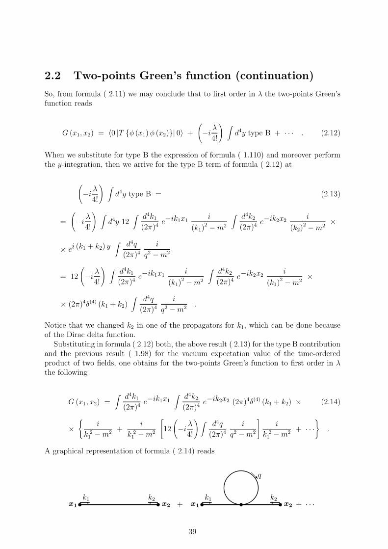
A graphical representation of formula ( 2.14) reads
x1 x2-k1 k2
+ x1 x2-k1 k2
@Rq
+ · · ·
39
2.3 Feynman rules (part II)
From formula ( 2.14) and its graphical representation one can read off further Feynmanrules for φ4 theory.
For each external point x, from which flows away momentum k, we have a Fourierintegration of the form
∫ d4k
(2π)4e−ikx . (2.15)
For overall momentum conservation we have a factor
(4π)4δ(4)(sum of the external momenta) . (2.16)
For each propagator in which flows momentum p we have a factor
i
p2 −m2 . (2.17)
For each internal point, usually referred to as vertex, one has a factor related to theexpansion parameter, or coupling constant, given by
−i λ4!
. (2.18)
From the series in formula ( 2.2) we learn moreover that a graph with s vertices bringsa factor (s!)−1 from the expansion of the exponent. Consequently, for a Feynman graphwith s vertices, also taking into account the factors ( 2.18), one has to include an overallfactor
1
s!
(
−i λ4!
)s. (2.19)
Then there is a combinatorial factor, which, for example, for the second term of ( 2.14),or the type B contribution, equals twelve as shown in formula ( 1.107).
And finally, for each internal loop, with loop momentum q, we find an integration ofthe form
∫ d4q
(2π)4. (2.20)
Following these Feynman rules, one determines all possible contributions to any n-pointGreen’s function for φ4 theory.
40
2.4 The second order in λ contribution to G (x1, x2)
In order to get some training in applying the Feynman rules which are discussed in section( 2.3), and to, moreover, discover new properties for the series expansion of an n-pointsGreen’s function, we determine here in all detail the second order, in the coupling constant,contributions to the two-points Green’s function.
A second order Feynman graph has two internal points and hence, following the Feyn-man rule ( 2.19), yields an overal factor
1
2!
(
−i λ4!
)2
Furthermore, since we are dealing with a two-points Green’s function, we have two Fourierintegrations of the form ( 2.15). Then, according to equation ( 2.11) we only need tofind the Feynman graphs without vacuum bubbles, for which the external points cannotbe contracted amongst each other. Consequently, each possible contribution has twoexternal propagators, or legs, for which the factors are given in Feynman rule ( 2.17).When we include moreover the factor ( 2.16), which guarantees momentum conservationfor the external momenta, then we find the following generic form for the second ordercontribution to the two-points Green’s function.
1
2!
(
−i λ4!
)2∫
d4k1(2π)4
e−ik1x1 i
k 21 −m2
∫
d4k2(2π)4
e−ik2x2 i
k 21 −m2 (2π)4 δ(4) (k1 + k2)
× something . (2.21)
Since in the expression for something we do not have to bother any more about theexternal legs, this is also called the amputed Green’s function.
As mentioned before, according to equation ( 2.11) we only need to find the Feynmangraphs without vacuum bubbles, in order to determine the something of formula ( 2.21).Below, we discuss the three graphically distinct possibilities.
1. The first second order contribution which comes to our mind has a graphical represen-tation which consists just of two times the type B Feynman graph for formula ( 1.108),i.e.
x1 x2
From the above graph we can read the combinatorial factor, which indicates how manydifferent contractions are possible. First, we can contract each of the two external pointsto any of the two internal points, which gives two possibilities. One external momentumcan be contracted to any of the four momenta from an internal point, which gives fourtimes four possiblities. Then, there are three momenta left at each vertex, which givesthree times three possibilities to contract any pair of them. So, in total we obtain
2 × 4 × 4 × 3 × 3 = 288 (2.22)
41
different ways for performing the contractions and still end up with the same graph, whichmeans that this graph represents 288 different, but analytically the same, contributions.
Besides the external propagators, which are already taken care of in expression ( 2.21),there are three more propagators, the two loops and the propagator which results fromthe contraction of the momenta of two different internal points. Momentum conservationdemands that the momentum, which flows in the propagator which connects the twointernal points, equals the external momenta, i.e. k1. For the two loop momenta weselect q1 and q2.
We find then the following contribution to the something of formula ( 2.21)
288
[
∫ d4q1(2π)4
i
q 21 −m2
]
i
k 21 −m2
[
∫ d4q2(2π)4
i
q 22 −m2
]
. (2.23)
Since, in fact, for this contribution there are no external legs involved, its correct graphicalrepresentation is given by
However, for the combinatorics it is easier to also consider the external legs.
2. The next second order contribution has the following Feynman graph.
x1 x2
As in the previous case, there are two different ways to connect the external points tothe internal points. Also the contraction of one external momentum to any of the fourvertex momenta can be done in four different ways and the same for the other externalmomentum. Each vertex has then three remaining momenta. For the first choice tocontract one momentum of one vertex with any of the three momenta of the other vertex,are three possibilities. For the second choice two ways. Whereas for the last choice onlyone possibility is left. So, we obtain as a result that this Feynman graph represents
2 × 4 × 4 × 3 × 2 × 1 = 192 (2.24)
different, though analytically the same, contributions.Besides the external propagators, which are already taken care of in expression ( 2.21),
there are three more propagators, each connecting the two different internal points. Letus take the momentum flow in those three propagators in the direction away from x1towards x2. Then, if one of those three propagators takes momentum q1, and a secondmomentum q2, the third, because of momentum conservation, must take k1− q1− q2. Forthe two loop momenta we select q1 and q2.
42
We find then the following contribution to the something of formula ( 2.21) for thiscase
192∫
d4q1(2π)4
∫
d4q2(2π)4
i
q 21 −m2
i
q 22 −m2
i
(k1 − q1 − q2)2 −m2. (2.25)
Since also for this contribution there are no external legs involved, its correct graphicalrepresentation is given by
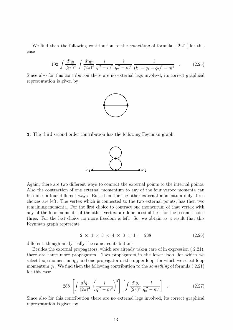
3. The third second order contribution has the following Feynman graph.
x1 x2
Again, there are two different ways to connect the external points to the internal points.Also the contraction of one external momentum to any of the four vertex momenta canbe done in four different ways. But, then, for the other external momentum only threechoices are left. The vertex which is connected to the two external points, has then tworemaining momenta. For the first choice to contract one momentum of that vertex withany of the four momenta of the other vertex, are four possibilities, for the second choicethree. For the last choice no more freedom is left. So, we obtain as a result that thisFeynman graph represents
2 × 4 × 3 × 4 × 3 × 1 = 288 (2.26)
different, though analytically the same, contributions.Besides the external propagators, which are already taken care of in expression ( 2.21),
there are three more propagators. Two propagators in the lower loop, for which weselect loop momentum q1, and one propagator in the upper loop, for which we select loopmomentum q2. We find then the following contribution to the something of formula ( 2.21)for this case
288
∫
d4q1(2π)4
(
i
q 21 −m2
)2
[
∫
d4q2(2π)4
i
q 22 −m2
]
. (2.27)
Since also for this contribution there are no external legs involved, its correct graphicalrepresentation is given by
43
The something of the second order, in λ, contribution ( 2.21) to the two-points Green’sfunction, is just the sum of the three above determined expressions, (2.23), (2.25), and(2.27).
When, one wants to be sure that no contribution has been forgotten, then one may alsotake the vacuum bubble diagrams of section ( 2.1) into account. The reason is, that thetotal number of possible contractions can easily be determined. There are ten momentaflowing from two external points, which contribute each one momentum, and from twointernal points, which contribute each four momenta. The first external momentum canbe contracted with any of the other nine momenta, the second with any of the remainingmomenta. One of the then six remaining momenta can be contracted in five differentways. One of the then four remaining momenta can be contracted in three different ways.For the last two momenta no more freedom exists. We find then
9 × 7 × 5 × 3 × 1 = 945 (2.28)
For the vacuum bubbles of section ( 2.1), in the order of appearance, one has the multiplic-ities 9, 72, 24, and 72 respectively. Summing those possible different ways of contractingthe momenta, to the numbers of formulas (2.22), (2.24), and (2.26), one finds
9 + 72 + 24 + 72 + 288 + 192 + 288 = 945 ,
which result agrees indeed with the total number given in formula ( 2.28).
44
2.5 The amputed Green’s function
For the two-points Green’s function ( 2.1), using formulas ( 2.14), ( 2.21), and the secondorder contributions (2.23), (2.25), and (2.27), we obtain to second order in λ the result
G (x1, x2) =x1 x2
+x1 x2
+x1 x2
+x1 x2
+x1 x2
+ · · ·
=∫
d4k1(2π)4
e−ik1x1∫
d4k2(2π)4
e−ik2x2 (2π)4δ(4) (k1 + k2) × (2.29)
×
i
k 21 −m2 +
i
k 21 −m2 F
(
k1, λ,m2) i
k 21 −m2
,
where F (k1, λ,m2) is the so-called amputed two-points Green’s function, given by
F (k1, λ,m2) = + + + + · · ·
= −iλ2
∫
d4q1(2π)4
i
q 21 −m2 + (2.30)
−λ2
4
[
∫
d4q1(2π)4
i
q 21 −m2
]
i
k 21 −m2
[
∫
d4q2(2π)4
i
q 22 −m2
]
+
−λ2
6
∫
d4q1(2π)4
∫
d4q2(2π)4
i
q 21 −m2
i
q 22 −m2
i
(k1 − q1 − q2)2 −m2+
−λ2
4
∫ d4q1(2π)4
(
i
q 21 −m2
)2
[
∫ d4q2(2π)4
i
q 22 −m2
]
+ · · · ,
Notice, that though the multiplicities for contributions of higher orders in λ are large,the factors for the powers of λ are moderate because of the factor 4! in the interactionLagrangian ( 1.36).
45
2.6 1PI graphs and the self-energy
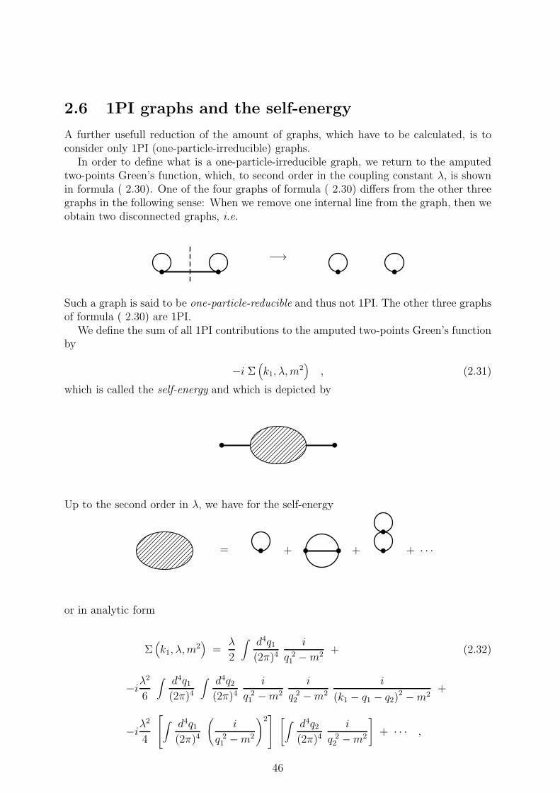
A further usefull reduction of the amount of graphs, which have to be calculated, is toconsider only 1PI (one-particle-irreducible) graphs.
In order to define what is a one-particle-irreducible graph, we return to the amputedtwo-points Green’s function, which, to second order in the coupling constant λ, is shownin formula ( 2.30). One of the four graphs of formula ( 2.30) differs from the other threegraphs in the following sense: When we remove one internal line from the graph, then weobtain two disconnected graphs, i.e.
−→
Such a graph is said to be one-particle-reducible and thus not 1PI. The other three graphsof formula ( 2.30) are 1PI.
We define the sum of all 1PI contributions to the amputed two-points Green’s functionby
−i Σ(
k1, λ,m2)
, (2.31)
which is called the self-energy and which is depicted by
Up to the second order in λ, we have for the self-energy
= + + + · · ·
or in analytic form
Σ(
k1, λ,m2)
=λ
2
∫ d4q1(2π)4
i
q 21 −m2 + (2.32)
−iλ2
6
∫
d4q1(2π)4
∫
d4q2(2π)4
i
q 21 −m2
i
q 22 −m2
i
(k1 − q1 − q2)2 −m2+
−iλ2
4
∫ d4q1(2π)4
(
i
q 21 −m2
)2
[
∫ d4q2(2π)4
i
q 22 −m2
]
+ · · · ,
46
Between the self-energy ( 2.31) and the amputed two-points Green’s function ( 2.30) canbe shown the following relation
F(
k, λ,m2)
=[
−iΣ(
k, λ,m2)]
+[
−iΣ(
k, λ,m2)] i
k2 −m2
[
−iΣ(
k, λ,m2)]
+ · · · .
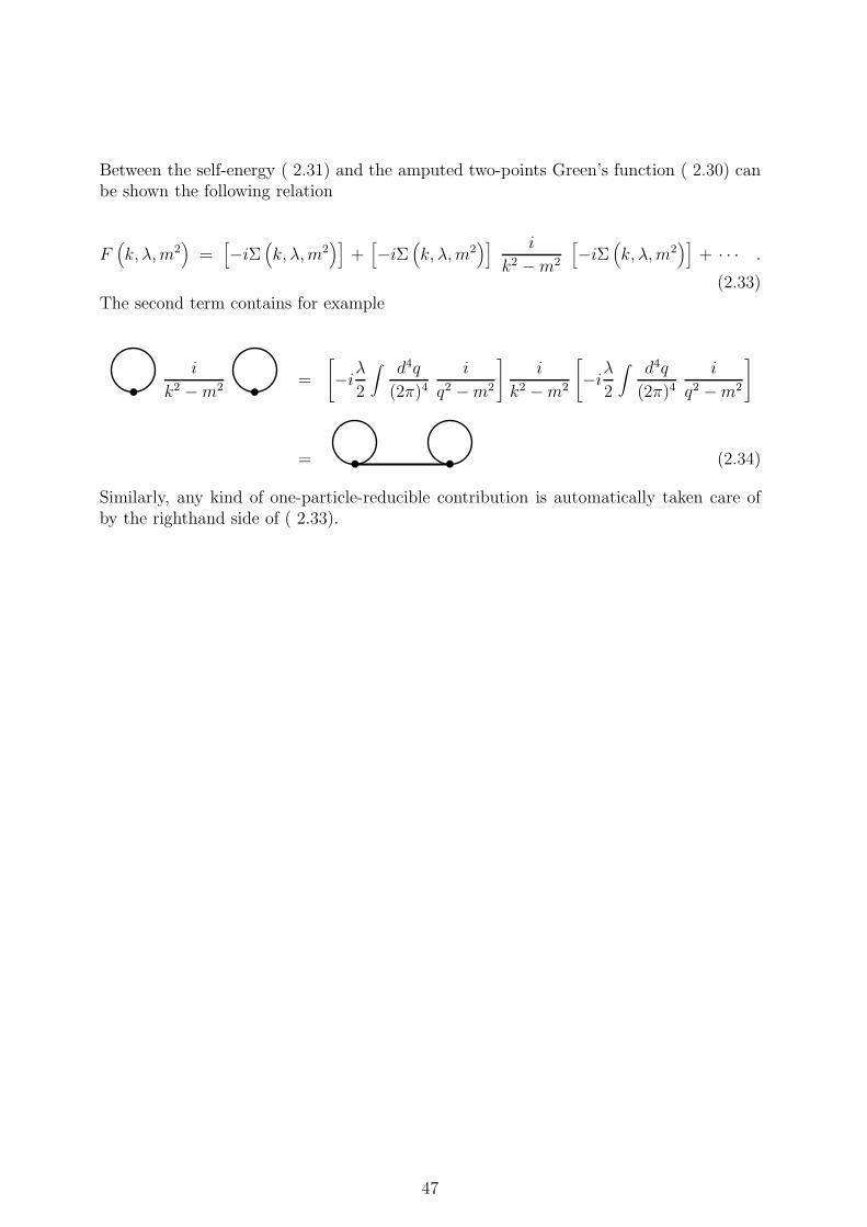
(2.33)The second term contains for example
i
k2 −m2 =
[
−iλ2
∫
d4q
(2π)4i
q2 −m2
]
i
k2 −m2
[
−iλ2
∫
d4q
(2π)4i
q2 −m2
]
= (2.34)
Similarly, any kind of one-particle-reducible contribution is automatically taken care ofby the righthand side of ( 2.33).
47
2.7 Full propagator
One might have noticed, for instance by inspection of formula ( 2.29), that for the freetheory, for which λ = 0 and hence for which the interaction Lagrangian of ( 1.34) isabsent, the two-points Green’s function ( 2.1) equals the vacuum expectation value of thetime-ordered product of two fields, given in formula ( 1.98). The central part of formula( 1.98) is the free propagator SF , which has been defined in equation ( 1.23). For thecentral part of the two-points Green’s function for the complete theory, we define the fullpropagator, S ′
F , i.e.
G (x, x′) =∫ d4k
(2π)4e−ikx
∫ d4k′
(2π)4e−ik
′x′ (2π)4δ(4) (k + k′) S ′F
(
k, λ,m2)
. (2.35)
The full propagator is graphically represented by
From formulas ( 1.23), ( 2.30), ( 2.33), and ( 2.35) one reads off the following relationbetween the full propagator, the free propagator and the self-energy, given by
= + + + · · ·
or using their symbolic notation, by
S ′F = SF + SF (−iΣ) SF + SF (−iΣ) SF (−iΣ) SF + · · · , (2.36)
which series can be formally summed and written in a compact form
S ′F
(
k, λ,m2)
=i
k2 −m2 − Σ (k, λ,m2). (2.37)
48
2.8 Divergencies
In the foregoing, we have obtained a beautiful analytic expression for the two-pointsGreen’s function in formulas ( 2.29) and ( 2.30). However, we still have not come veryfar, since the loop integrals are divergent and hence the whole expression does not exist.But, would we discuss a theory which does not lead to any sensible result? Of course not!
There exist several regularization methods to get rid of the infinities, which accompanyalmost any quantum field theory (see, for example Bjorken and Drell, chapters 8 and 19,or Itzykson and Zuber, chapter 8). Here, we will study an elegant procedure, which isdeveloped by G. ’t Hooft and M. Veltman. Although we need then the concept of non-integer dimensions, this is no problem since all relevant integrals in arbitrary dimensionsare tabulated. In appendix B of Diagrammar, or appendix A of their Nuclear Physicsarticle, G. ’t Hooft and M. Veltman give (see also section 2.8.1)
∫
dnp1
p2 +m2 =iπ
1
2n
(m2)1− 1
2nΓ(
1− 1
2n)
. (2.38)
However, their metric differs from ours, i.e.
p2 =
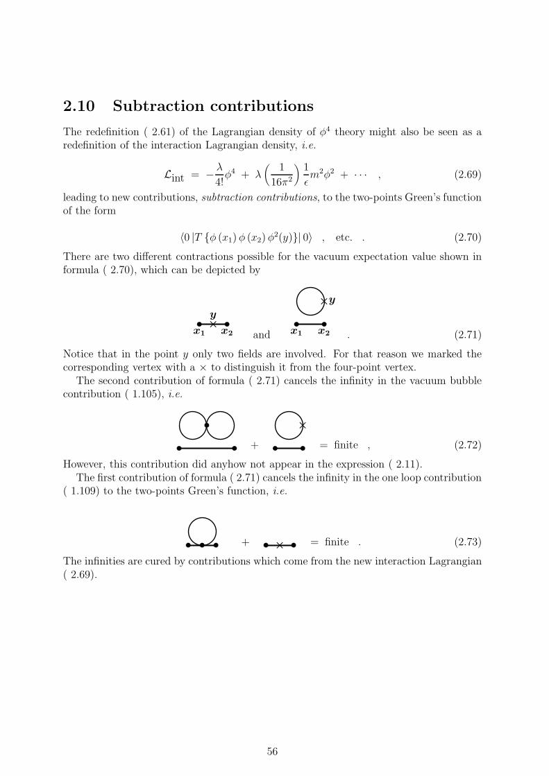
−E2 + ~p 2 (G. ’t Hooft and M. Veltman)
+E2 − ~p 2 (our definition.)(2.39)
Consequently, in our definition of the metric we obtain for formula ( 2.38) the followingresult
∫
dnqi
q2 −m2 =π
1
2n
(m2)1− 1
2nΓ(
1− 1
2n)
. (2.40)
Γ represents the gamma function, which is an extension to complex values of the factorialfunction and which has the following property
Γ(α+ 1) = αΓ(α) . (2.41)
Notice that as a consequence of this property, Γ(0), Γ(−1), Γ(−2), Γ(−3), . . ., do not exist(are infinite) and hence for 4-dimensional physics (i.e. n = 4), formula ( 2.40) diverges.
The divergent integral which contributes to the first order in λ term of the self-energy( 2.32) is exactly given by formula ( 2.40) for n = 4. The limit n = 4 does not exist,because Γ(−1) does not exist. However, we define ǫ = n− 4, in order to obtain
∫
d4qi
q2 −m2 = limǫ→0
π2+ 1
2ǫ
(m2)−1− 1
2ǫΓ(
−1 − 1
2ǫ)
. (2.42)
The gamma function we might handle by using the property ( 2.41), which leads to
Γ(
−1 − 1
2ǫ)
=Γ(
−12ǫ)
−1− 12ǫ
,
and moreover the Laurent series expansion (see for example M.Abramowitz and I. Stegun,Handbook of Mathematics, formula 6.1.35) for the gamma function in the neighborhoodof zero, i.e.
49
Γ(α) =1
α+ finite part ,
where the finite part does not contain infinities in the limit α→ 0.So, when we forget about the limit (ǫ → 0), but keep it in mind, then we find for
expression ( 2.42), the result
∫
d4qi
q2 −m2 = π2m2
2
ǫ+ finite part
. (2.43)
Now, the expression ( 2.32) for the self-energy, which is an expansion in the couplingconstant λ, has the following structure
Σ = λΣ1 + λ2Σ2 + · · · (2.44)
where
λΣ1 = (one loop) and λ2Σ2 = + (two loops)
Here, we are studying the regularization procedure up to one loop term(s), for whichit suffices to consider from the above expansion ( 2.44) only
Σ = λΣ1 + · · ·
=λ
2
∫
d4q
(2π)4i
q2 −m2 + · · ·
= λ m2(
1
16π2
)
1
ǫ+ finite part
(2.45)
2.8.1 Integration in n dimensions
In an n dimensional Euclidean space we assume Cartesian coordinates
x(n)i , i = 1, . . . , n
and define spherical coordinates through
x(n)1 = r sin (ϑn−1) · · · sin (ϑ4) sin (ϑ3) sin (ϑ2) sin (ϑ1)
x(n)2 = r sin (ϑn−1) · · · sin (ϑ4) sin (ϑ3) sin (ϑ2) cos (ϑ1)
x(n)3 = r sin (ϑn−1) · · · sin (ϑ4) sin (ϑ3) cos (ϑ2)
Relation (2.48) can be proven by means of induction. For n = 1 one has x1 = r anddx = dr, for n = 2 one has, employing the usual cylindrical coordinates r and ϕ, thatd2x = rdr dϕ, whereas moreover, for n = 3, with the ordinary three-dimensional sphericalcoordinates r, ϑ and ϕ, one has d3x = r2dr sin (ϑ) dϑ dϕ, all in agreement with formula(2.48).
For (n + 1) dimensions we define the spherical coordinates through
x(n+1)i = x
(n)i sin (ϑn) for i 6= n + 1
x(n+1)n+1 = r cos (ϑn) . (2.49)
Hence, when we define the Jacobian in n dimensions by
J(n) =
∣
∣
∣
∣
∣
∣
∣
∣
∣
∣
∣
∣
∣
∣
∣
∣
∣
∣
∣
∂x(n)1∂r
∂x(n)1
∂ϑ1· · · ∂x
(n)1
∂ϑn−1
∂x(n)2∂r
· · · · · · · · ·...
......
...
∂x(n)n∂r
∂x(n)n∂ϑ1
· · · ∂x(n)n∂ϑn−1
∣
∣
∣
∣
∣
∣
∣
∣
∣
∣
∣
∣
∣
∣
∣
∣
∣
∣
∣
, (2.50)
then we obtain in (n+ 1) dimensions for the Jacobian the form
J(n+ 1) =
∣
∣
∣
∣
∣
∣
∣
∣
∣
∣
∣
∣
∣
∣
∣
∣
∣
∣
∣
∣
∣
∣
∣
∣
∣
∣
∣
∣
∣
∣
sinn (ϑn) J(n)
∣
∣
∣
∣
∣
∣
∣
∣
∣
∣
∣
∣
x(n)1 cotg (ϑn)
x(n)2 cotg (ϑn)
...
x(n)n cotg (ϑn)cos (ϑn) 0 · · · 0 −r sin (ϑn)
∣
∣
∣
∣
∣
∣
∣
∣
∣
∣
∣
∣
∣
∣
∣
∣
∣
∣
. (2.51)
The first n elements of the last column of this determinant are equal to the first n elementsof the first column, multiplied by a factor
rcos (ϑn)
sin2 (ϑn).
Consequently one has the relation
J(n + 1) = r cotg (ϑn) cos (ϑn) + r sin (ϑn) sinn (ϑn) J(n)
= r sinn−1 (ϑn) J(n) . (2.52)
51
The above result (2.52) combined with formula (2.48), gives then
which proofs formula (2.48).For integrands which are functions of x2 only, one may perform the integrals over the
angles independently. So, let us next concentrate on the following integral
Im =∫ π
0dϑ sinm (ϑ) . (2.54)
Integration by parts gives
Im =m− 1
mIm−2 ,
which can be iterated. For even values of m one finds
I2k =2k − 1
2kI2k−2 = · · · = (2k − 1)(2k − 3) · · ·1
2k(2k − 2) · · ·2 I0 =Γ(
k + 12
)
/Γ(
12
)
Γ (k + 1)π .
Whereas, for odd values of m one finds
I2k+1 =2k
2k − 1I2k−1 = · · · = 2k(2k − 2) · · ·2
(2k + 1)(2k − 1) · · ·3 I1 =Γ (k + 1)
Γ(
k + 32
)
/Γ(
32
) 2 .
Both cases can be written in the same way, by
Im =√πΓ(
12(m+ 1)
)
Γ(
12m+ 1
) . (2.55)
With expression (2.55) we are ready for the integrals over the angles. One obtains
∫ π
0sinn−2 (ϑn−1) dϑn−1
∫ π
0sinn−3 (ϑn−2) dϑn−2 · · ·
∫ π
0sin (ϑ2) dϑ2
∫ 2π
0dϑ1 =
=√πΓ(
12(n− 1)
)
Γ(
12n)
√πΓ(
12(n− 2)
)
Γ(
12(n− 1)
) · · · √π Γ (1)
Γ(
32
) 2π = 2π
12n
Γ(
12n) . (2.56)
For the radial part of integration (2.38), we consider Euler’s integral of the first kind, orBeta function, defined by
Γ(x)Γ(y)
Γ(x+ y)= B(x, y) =
∫ ∞
0dt
tx−1
(t + 1)x+y . (2.57)
Hence,
52
∫
dnr1
r2 + 1=
∫ ∞
0rn−1dr
1
r2 + 1
∫
angles = 12
∫ ∞
0dtt12n−1
t+ 1
∫
angles
= B(
12n , 1− 1
2n)
∫
angles = π12n Γ
(
1− 12n)
. (2.58)
In formula (2.38) p2 is defined by
p2 = − p02 + ~p 2 . (2.59)
In order to obtain an Euclidean integral, we introduce
p0 = i pn , (2.60)
which explains the i in formula (2.38).
53
2.9 Counterterms
Suppose that, instead of the Lagrangian density ( 1.34), we had chosen for a theory withthe Lagrangian density given by
L(
φ, ∂µ φ)
=1
2
(
∂µ φ)2 − 1
2Bm2φ2 − λ
4!φ4 , (2.61)
where B is called a counterterm. Then, in the theory ( 2.61), we would obtain for the freepropagator not the Feynman propagator ( 1.23), but instead
SF (p) =i
p2 −Bm2 , (2.62)
and, consequently, up to first order terms in λ for the self-energy, not expression ( 2.45),but instead
Σ = λ Bm2(
1
16π2
)
1
ǫ+ finite part
(2.63)
For the full propagator S ′F we would have found, not expression ( 2.37), but, to first order
in λ, instead
S ′F =
i
k2 − Bm2 − λ Bm2
(
116π2
)
1ǫ + finite part
. (2.64)
The counterterm B of the Lagrangian density ( 2.61) is supposed to also be expandablein a series of increasing orders of λ, like the self-energy ( 2.44), i.e.
B = 1 + λb1 + λ2b2 + · · · . (2.65)
Now, since we are only interested in terms up to order λ, we have for the second term inthe denominator of the righthand side of formula ( 2.64)
Bm2 = m2 + λb1m2 + · · · ,
and for the third term
λ Bm2(
1
16π2
)
1
ǫ+ finite part
= λm2(
1
16π2
)
1
ǫ+ finite part
.
So, the full propagator up to first order in λ yields
S ′F =
i
k2 −m2 − λ m2
b1 +(
116π2
)
1ǫ + finite part
. (2.66)
The obvious choice
b1 = −(
1
16π2
)
1
ǫ, (2.67)
leads to a finite expression for the full propagator
S ′F =
i
k2 −m2 − λ m2 finite part . (2.68)
54
This procedure is essentially the regularization method. One modifies the Lagrangiandensity, order by order in λ, in such a way that the the Green’s functions become finite.The divergencies are absorbed in the definition of the counterterms. Lagrangian densitiesfor which this procedure works, are called renormalizable. From electromagnetism, whereone has the famous calculations for the anomalous magnetic moment of the electron andthe Lamb shift of the Hydrogen atom, for which the regularization procedure gives veryaccurate agreement of the predictions with experiment, we know that the method works!
55
2.10 Subtraction contributions
The redefinition ( 2.61) of the Lagrangian density of φ4 theory might also be seen as aredefinition of the interaction Lagrangian density, i.e.
Lint = − λ4!φ4 + λ
(
1
16π2
)
1
ǫm2φ2 + · · · , (2.69)
leading to new contributions, subtraction contributions, to the two-points Green’s functionof the form
〈0 |T φ (x1)φ (x2)φ2(y)| 0〉 , etc. . (2.70)
There are two different contractions possible for the vacuum expectation value shown informula ( 2.70), which can be depicted by
x1 x2
×y
and x1 x2
×y
. (2.71)
Notice that in the point y only two fields are involved. For that reason we marked thecorresponding vertex with a × to distinguish it from the four-point vertex.
The second contribution of formula ( 2.71) cancels the infinity in the vacuum bubblecontribution ( 1.105), i.e.
+
×
= finite , (2.72)
However, this contribution did anyhow not appear in the expression ( 2.11).The first contribution of formula ( 2.71) cancels the infinity in the one loop contribution
( 1.109) to the two-points Green’s function, i.e.
+ × = finite . (2.73)
The infinities are cured by contributions which come from the new interaction Lagrangian( 2.69).
56
Chapter 3
Four-points Green’s function
Let us, for a moment, return to the unregularized Lagrangian ( 1.34) and determine thefour points Green’s function, which, by virtue of equation ( 1.37), is given by
G (x1, x2, x3, x4)⟨
0
∣
∣
∣
∣
T
exp[
i∫
d4y(
− λ4!)
φ4(y)]
(φ(y))∣
∣
∣
∣
0⟩
=
= 〈0 |T φ (x1)φ (x2)φ (x3)φ (x4)| 0〉 +
+⟨
0
∣
∣
∣
∣
T
φ (x1)φ (x2)φ (x3)φ (x4) i∫
d4y(
− λ4!)
φ4(y)∣
∣
∣
∣
0⟩
+
+
⟨
0
∣
∣
∣
∣
∣
T
φ (x1)φ (x2)φ (x3)φ (x4)12
[
i∫
d4y(
− λ4!)
φ4(y)]2∣
∣
∣
∣
∣
0
⟩
+ · · · .(3.1)
As for the two points Green’s function, it is easy to demonstrate that also in this casethe vacuum bubble graphs do not contribute to the four points Green’s function. In thefollowing, we will not determine order by order each of the terms of the perturbationseries expansion of formula ( 3.1). But, rather select classes of series of contributions tothe four points Green’s function, such that for each class it is perfectly transparant ofhow to proceed in order to calculate the various terms in those series. This facilitates thebookkeeping and in particular makes it more obvious to understand how the regularizationprocedure works. We begin by the zeroeth order terms of the series expansion ( 3.1) andstudy the classes of graphs which are associated to them. Then, we select a particular termfrom the first order contributions, the vertex contribution, and show how the remaininggraphs, which together with the vertex constitute the vertex function, are associated tothat expression and, in particular, how the regularization method works for that vertexfunction.
The zeroeth order term in the coupling constant λ is just the vacuum expectation valuefor the time ordered product of four fields, which has been studied in section ( 1.7) andexplicitly given by the sum of formulas ( 1.91), ( 1.92), and ( 1.93) and represented bythe corresponding graphs. Let us here concentrate on one of the three contributions, forexample the one given by formula ( 1.91):
57
•
•
•
•
x3
x1
x4
x2
= i2∫
d4k1(2π)4
e−ik1 (x1 − x2)(k1)
2 −m2
∫
d4k3(2π)4
e−ik3 (x3 − x4)(k3)
2 −m2. (3.2)
The expression for the above contribution ( 3.2) can also be casted in the general form,i.e. in the form which follows from the Feynman rules, according to
[
4∏
ℓ=1
∫
d4kℓ(2π)4
e−ikℓxℓ]
(2π)4 δ(4)(
4∑
ℓ=1
kℓ
)
(2π)4 δ(4) (k1 + k2)i
(k1)2 −m2
i
(k3)2 −m2
.
(3.3)The central part of contribution ( 1.91) is hence given by
(2π)4 δ(4) (k1 + k2)i
(k1)2 −m2
i
(k3)2 −m2
. (3.4)
Next to the contribution ( 3.2), there exists a class of contributions to the four pointsGreen’s function ( 3.1) which can easily be summed up, i.e. the following series
+ + + + + · · ·
Using formula ( 2.35), in which the full propagator, S ′F , is defined, we can write the
full sum of the above depicted contributions by
= (2π)4 δ(4) (k1 + k2) S′F
(
k1, λ,m2) i
(k3)2 −m2
. (3.5)
One can extend this class of contributions by considering also all higher order in λcontributions to the lower propagator, i.e.
58
+ + · · · =
which represent all possible contributions one may think of for which the general structureis equivalent to ( 1.91), i.e. momentum flows from x1 to x2 and also from x3 to x4, butthere are no lines which connect the upper full propagator to the lower full propagator.In formule, the central part of this total class of contributions is given by
(2π)4 δ(4) (k1 + k2) S′F
(
k1, λ,m2)
S ′F
(
k3, λ,m2)
. (3.6)
Following the same procedure for the contributions ( 1.92) and ( 1.93), we obtain forthe four points Green’s function the expression
G (x1, x2, x3, x4) =
[
4∏
ℓ=1
∫ d4kℓ(2π)4
e−ikℓxℓ]
(2π)4 δ(4)(
4∑
ℓ=1
kℓ
)
×
(2π)4 δ(4) (k1 + k2) S′F
(
k1, λ,m2)
S ′F
(
k3, λ,m2)
+ (3.7)
+ (2π)4 δ(4) (k1 + k3) S′F
(
k1, λ,m2)
S ′F
(
k2, λ,m2)
+
+ (2π)4 δ(4) (k1 + k4) S′F
(
k1, λ,m2)
S ′F
(
k3, λ,m2)
+
+ other higher order terms in λ .
It might be clear that, once the full propagator, S ′F , is regularized, then the first three
terms of the righthand side of the expansion ( 3.7), which actually already represent aninfinity of contributions of three special types, are automatically also regularized. So, letus concentrate on the other higher order in λ contributions.
3.1 The vertex
The first order in λ term from the perturbation expansion ( 3.1) reads
i∫
d4y
(
− λ4!
)
〈0 |T φ (x1)φ (x2)φ (x3)φ (x4) φ4(y)| 0〉 . (3.8)
Here, we do not have to consider the vacuum bubble contributions, which are contractionsof the external momenta, k, which originate from the external events, x, amongst them-selves and of the internal momenta, q, which originate at the internal event, y, amongstthemselves. The contribution which is graphically represented by
59
is already contained in the series ( 3.6) and hence does not have to be considered again.The other one-particle irreducible graph occurs by the contraction of the four internal
momenta, q, which originate from the internal event, y, each with one of the externalmomenta, i.e.
This is a new type of contribution and is called the vertex. Its combinatorial factor equals4!, which compensates exactly the factor 1/4! from the interaction Lagrangian ( 1.36).
One can associate a whole class of contributions for ( 3.1), by substitution of thefour external propagators by full propagators. This class of contributions is graphicallyrepresented by the following figure.
x1 x2
x3x4
Apart from the factors 4π and the delta function, one obtains for this series the expression
4!
(
−i λ4!
)
S ′F
(
k1, λ,m2)
S ′F
(
k2, λ,m2)
S ′F
(
k3, λ,m2)
S ′F
(
k4, λ,m2)
. (3.9)
Once S ′F is regulated, this whole class of contributions is consequently also regulated.
3.2 The second order terms
Besides contributions, which are already contained in the sums of contributions ( 3.6) or( 3.9), one has the following one-particle irreducible graphs
60
x1 x2
x3x4
,
x1 x2
x3x4
and
x1 x2
x3x4
(3.10)
Let us concentrate on the first of the three contributions to ( 3.1). The combinatoricslearns us that there are (4!)2 ways to make such contractions that the final result has thesame analytic appearance. This factor just cancels the same, but inverted, factor fromthe interaction Lagrangian. So, apart from the factors 4π and the delta function, oneobtains for this contribution the expression
(4!)21
2!
[
4∏
ℓ=1
i
k 2ℓ −m2
](
−i λ4!
)2∫
d4q
(2π)4i
q2 −m2
i
(k1 + k2 − q)2 −m2. (3.11)
To this contribution we can also associate a whole class of contributions, by just sub-stituting the four external propagators by full propagators. The total sum of this class ofcontributions gives the result
[
4∏
ℓ=1
S ′F
(
kℓ, λ,m2)
]
1
2(−iλ)2
∫
d4q
(2π)4i
q2 −m2
i
(k1 + k2 − q)2 −m2. (3.12)
The expression ( 3.12) could be seen as one of the first order in λ correction to the sumof contributions of formula ( 3.9), because for each term of the sum of contributions tothe four points Green’s function, which is represented by formula ( 3.9), a correspondingterm with one more internal vertex is contained in formula ( 3.12). The other two firstorder in λ corrections to the sum of contributions of formula ( 3.9) are obtained, similarly,by substitution of the external propagators of the other two graphs of formula ( 3.10).
3.3 The amputed vertex function
When we sum up the class extensions of the vertex, formula ( 3.9), the class extension ofthe first first order in λ correction to the vertex, formula ( 3.12), and the class extensionof the other two graphs in formula ( 3.10), then we obtain the vertex function, given by
[
4∏
ℓ=1
S ′F
(
kℓ, λ,m2)
]
(−iλ) +1
2(−iλ)2
∫
d4q
(2π)4i
q2 −m2
i
(k1 + k2 − q)2 −m2+
61
+1
2(−iλ)2
∫
d4q
(2π)4i
q2 −m2
i
(k1 + k3 − q)2 −m2+
+1
2(−iλ)2
∫ d4q
(2π)4i
q2 −m2
i
(k1 + k4 − q)2 −m2+ · · ·
, (3.13)
which is graphically represented by the figure below
x1 x2
x3x4
The central expression which we will consider here, is called the amputed vertex func-tion, which is given by
Λ(
k1, k2, k3, k4, λ,m2)
= (3.14)
= (−iλ) +1
2(−iλ)2
∫
d4q
(2π)4i
q2 −m2 ×
×
i
(k1 + k2 − q)2 −m2+
i
(k1 + k3 − q)2 −m2+
i
(k1 + k4 − q)2 −m2+ · · ·
,
and which is graphically represented by
Any contribution to the four-points Green’s function belongs either to the first threeterms of expression ( 3.7), which represent two disconnected full propagators, or to theclass of contributions ( 3.13).
62
3.4 Regularization of the vertex function
The expression ( 3.14) for the amputed vertex function contains infinities, since
1
2
∫
d4q
(2π)41
(q2 −m2) ((k − q)2 −m2)= −i
(
1
16π2
)
1
ǫ+ finite parts
. (3.15)
And, since moreover, formula ( 3.14) contains three such integrals, we obtain, using theabove equation ( 3.15), for the amputed vertex function the expression
Λ(
k1, k2, k3, k4, λ,m2)
= −iλ− iλ2(
3
16π2
)
1
ǫ+ finite parts
. (3.16)
The regularization procedure works in a similar way as for the two-points Green’sfunction, in which case we defined a counterterm B to redefine the Lagrangian density(formula ( 2.61)), such that the new Lagrangian density gives finite results for the fullpropagator (formula ( 2.68)). Here we define the counterterm A, for which we assume theexpansion, given by
A = 1 + a1λ + a2λ2 + · · · , (3.17)
and redefine the Lagrangian density ( 2.61) to also include this counterterm, i.e.
L(
φ, ∂µ φ)
=1
2
(
∂µ φ)2 − 1
2Bm2φ2 − A
λ
4!φ4 . (3.18)
The amputed vertex function, for which we have the divergent expression ( 3.16), takesfor the Lagrangian density ( 3.18) the form
Λ = −iAλ− i(Aλ)2(
3
16π2
)
1
ǫ+ finite parts
= −iλ[
A + A2λ(
3
16π2
)
1
ǫ+ finite parts
]
. (3.19)
When the expression inside the square brackets of formula ( 3.19) is expanded to firstorder in λ, then we obtain
Λ = −iλ[
1 + a1λ + λ(
3
16π2
)
1
ǫ+ finite parts
]
, (3.20)
which upon the obvious choice
a1 = −(
3
16π2
)
1
ǫ
regulates the amputed vertex function to the ”first” order perturbation in λ
Λ = −iλ [1 + λ finite parts] , (3.21)
Notice that the vertex function, which is intimately related to the interaction part ofthe Lagrangian density, is proportional with the coupling constant λ. The first order inλ corrections yield thus terms quadratic in λ.
63
Chapter 4
Molding time evolution into a pathintegral
The concept of the path integral is rather easy to percieve. But, the precise mathematicalformulation of it, is a very complicated matter. Here, we will present a fast introduction,with just the minimum of complexity, avoiding most of the mathematical rigor.
The basic idea is that the time evolution of a system can be determined by inspectingall possible ways in which the system can evolve. Each possibility is called a path, likein classical mechanics. To each path is associated a probability, or more accurately, anamplitude. The central expression will turn out to be a sum, or integral, over all possiblepaths, of the amplitudes. In quantum mechanics this path integral has the followingappearance:
∫ x(tb)
x(ta)[dx(t)] ei Scl(x(t))/h . (4.1)
It assumes that the system evolves from a certain state (position in classical mechanics)x(ta) at the initial time ta to a state x(tb) at a later time tb. The symbol
∫
[dx(t)] indicatesthat the path integral is a sum over all possible paths, whereas the integration limits, x(ta)and x(tb), indicate that only those paths contribute to the integration, which at initialtime ta are in the state x(ta) and at the later time tb in the state x(tb). The amplitudefor each path is in expression (4.1) given by the exponent of the classical action Scl(x(t))for the path multiplied by i/h. Consequently, the amplitude is just a phase factor.
Adding phase factors is a subject which is studied in optics, where we learned aboutconstructive and destructive interference. Here, let us study expression (4.1) for subsets ofpossible paths which differ very little from each other. When for such a subset of nearbypaths the phases, which are measured in units h go through large changes, then theinterference is destructive. Consequently, such subset will not contribute much (basicallynothing) to the path integral. However, near an extremum of Scl(x(t)), the phases ofsubsets of paths will change very little. In that case one finds constructive interference.We may thus conclude that the main contribution to the path integral (4.1) stems fromthat subset of all possible paths which is near an extremum of the classical action.
The main issue, however, is not the calculation of the path integral itself, but merelythe measurable quantities which can be extracted from it. In the following we will studyhow path integrals may be constructed.
64
4.0.1 Time evolution in Quantum Mechanics
We assume that the dynamics of the system is described by a time-independent Hamil-tonian H , for which one may integrate the wave equation
i∂
∂t|ψ(t)〉 = H|ψ(t)〉 , (4.2)
to yield
|ψ(t)〉 = e−iHt|ψ(0)〉 (t > 0) . (4.3)
We also assume that the Hamiltonian H can be expressed in terms of the coordinateoperator q and the momentum operator p. The eigenstates of q are denoted |x(t)〉 and ofp by |k(t)〉. Wavefunctions are denoted by
ψ(x, t) = 〈x(t) |ψ(t)〉 , (4.4)
whereas in momentum space one has
ϕ(k, t) = 〈k(t) |ψ(t)〉 . (4.5)
We normalize the position and momentum eigenstates such that
〈k(t) |x(t′ )〉 =1√2π
e−ik(t)x(t′ ) . (4.6)
By applying relation (4.3), one obtains from equation (4.4) for the time evolution ofthe wave function the following
ψ(x, t) =⟨
x(t)
∣
∣
∣
∣
e−iH(t− t′ )∣
∣
∣
∣
ψ(t′ )⟩
(t > t′ )
=∫
dx(t′ )⟨
x(t)∣
∣
∣
∣
e−iH(t− t′ )∣
∣
∣
∣
x(t′ )⟩
〈x(t′ ) |ψ(t′ )〉
=∫
dx(t′ )⟨
x(t)
∣
∣
∣
∣
e−iH(t− t′ )∣
∣
∣
∣
x(t′ )⟩
ψ(x, t′ ) , (4.7)
The expression⟨
x(t)
∣
∣
∣
∣
e−iH(t− t′ )∣
∣
∣
∣
x(t′ )⟩
is called the full propagator, or Feynman kernel and contains the full information on howthe system develops in time from instant t′ to a later instant t. Relation (4.7) says thatfull knowledge of the wave function at instant t′ and full knowledge of the way the wavefunction propagates through space in the time interval from t′ to t, permits us to fullyreconstruct the wave function at instant t. This is called the Huyghens principle.
Here we will concentrate on a time interval which starts at instant ta and ends at alater instant tb, in order to determine an expression for the full propagator in terms ofclassical quantities. An intuitive way to arrive at such expression is shown by Feynmanand Hibbs. Here, we will closely follow their approach.
First, the time interval (ta, tb) is subdivided in N equal intervals, according to
t0 = ta, t1 = ta +∆t, t2 = ta + 2∆t, . . . , tN−1 = ta + (N − 1)∆t, tN = ta +N∆t = tb(4.8)
Next, we insert the identity operator, using completeness of the position eigenstates⟨
x(tb)∣
∣
∣
∣
e−iH(tb − ta)∣
∣
∣
∣
x(ta)⟩
= (4.10)
= 〈x(tb)| e−iH∆t∫
dx(tN−1) |x(tN−1)〉〈x(tN−1)| e−iH∆t
∫
dx(tN−2) |x(tN−2)〉〈x(tN−2)| . . .
. . .∫
dx(t2) |x(t2)〉〈x(t2)| e−iH∆t∫
dx(t1) |x(t1)〉〈x(t1)| e−iH∆t |x(ta)〉
=∫
dx(tN−1)∫
dx(tN−2) . . .∫
dx(t2)∫
dx(t1)⟨
x(tb)∣
∣
∣ e−iH∆t∣
∣
∣ x(tN−1)⟩
⟨
x(tN−1)∣
∣
∣ e−iH∆t∣
∣
∣ x(tN−2)⟩
. . .⟨
x(t2)∣
∣
∣ e−iH∆t∣
∣
∣x(t1)⟩⟨
x(t1)∣
∣
∣ e−iH∆t∣
∣
∣x(ta)⟩
In the limit N →∞, the resulting expression becomes the path integral form for the fullpropagator over all possible paths from x(ta) at instant ta to x(tb) at instant tb, since bytaking all possible values for x(ti) (i = 1, . . . , N − 1) by integration, one constructs allpossible paths.
However, it should be remarked that it is not at all clear yet whether such limit exists.Here, we do not further specify under which circumstances it is possible to take the limit.Instead, we assume that for the cases of interest to us, it can be done. Many textbooksdiscuss particular examples of Hamiltonians which allow a suitable definition of the pathintegral. But, even then, it is not completely straightforward.
Before proceeding, we will first evaluate one of the terms in the product which formsthe integrand of formula (4.10).
One term of the product in 4.10
In this intermezzo we study just one of the terms in the product of the integrand informula (4.10).
We start by once more inserting unity, this time by using completeness of the momen-tum eigenstates, i.e.
⟨
x(tn+1)∣
∣
∣ e−iH∆t∣
∣
∣ x(tn)⟩
= (4.11)
= 〈x(tn+1)|∫
dk(tn) |k(tn)〉〈k(tn)| e−iH∆t |x(tn)〉
66
=∫
dk(tn) 〈x(tn+1) |k(tn)〉⟨
k(tn)∣
∣
∣ e−iH∆t∣
∣
∣x(tn)⟩
As stated before, we assume that the HamiltonianH is built of position and momentumoperators, respectively q and p. Here, we assume furthermore that H is in the normalform, i.e. that momentum operators come to the left of all position operators. Thisis a reasonable assumption, since most expressions can be brought into such form. Forexample:
In the case H has the normal form, also using relation (4.6), we obtain
〈k |H(p, q)|x〉 = Hcl(k, x)〈k |x〉 = Hcl(k, x)1√2π
e−ikx . (4.12)
The classical Hamiltonian Hcl is a function of real numbers x(t) and k(t), not of operators.Now, it is generally not true that formula (4.12) can be extended to the exponent of
formula (4.11). But, for small enough ∆t, one may approximate
⟨
k(tn)∣
∣
∣ e−iH∆t∣
∣
∣ x(tn)⟩
≈ 〈k(tn) |(1− iH∆t)|x(tn)〉
=(
1− iHcl(k(tn), x(tn))∆t)
〈k(tn) |x(tn)〉
≈ e−iHcl(k(tn), x(tn))∆t 〈k(tn) |x(tn)〉 . (4.13)
A more elaborate approach can be found in chapter 3 of George Sterman’s book.Hence, also using formula (4.6) and its complex conjugate, for expression (4.11) we
where we also used x(tn+1) = x(tn +∆t).Anticipating moreover the limit for ∆t ↓ 0, we may write
⟨
x(tn+1)∣
∣
∣ e−iH∆t∣
∣
∣x(tn)⟩
= (4.15)
=1
2π
∫
dk(tn) ei∆t
[
k(tn) x(tn) − Hcl(k(tn), x(tn))]
.
Furthermore, for Hamiltonians of the type
H(p, q) =p2
2m+ V (q)
67
one obtains an integral of the Gaussian form,
∫ ∞
−∞dk e−αk2 + βk =
√
(
π
α
)
eβ2/4α . (4.16)
Consequently, we can perform the integral in formula (4.15), to find
⟨
x(tn+1)∣
∣
∣ e−iH∆t∣
∣
∣x(tn)⟩
= (4.17)
=
√
(
m
2πi∆t
)
ei∆t
[
m2 x2(tn) − V (x(tn))
]
√
(
m
2πi∆t
)
ei∆t Lcl(x(tn), x(tn)) ,
where Lcl is the classical Lagrangian for the system.
Back to formula 4.10
Substitution of the result (4.17) in formula (4.10), leads to
⟨
x(tb)
∣
∣
∣
∣
e−iH(tb − ta)∣
∣
∣
∣
x(ta)⟩
= (4.18)
=(
m
2πi∆t
)N/2 ∫
dx(tN−1) . . .∫
dx(t1)
ei∆t
[
Lcl(x(t1), x(t1)) + . . .+ Lcl(x(tN−1), x(tN−1))]
.
Formula (4.18) is the configuration space path integral. It is less general than the phasespace path integral, where both the integrations over x and k are kept.
In general, the limit N → ∞ might not exist. For some cases it can be shown that asuitable limit can be taken. One obtains then.
⟨
x(tb)
∣
∣
∣
∣
e−iH(tb − ta)∣
∣
∣
∣
x(ta)⟩
= (4.19)
=∫ x(tb)
x(ta)[dx(t)] ei
∫ tbta dt Lcl(x(t), x(t)) =
∫ x(tb)
x(ta)[dx(t)] ei Scl(x(t)) ,
where Scl represents the classical action for the system.The symbol
∫
[dx(t)] stands for the integral over all possible paths. The normalizationfactors have been absorbed into it.
68
69
Chapter 5
A path integral for fields
For fields φ one may define a path integral by summing over all possible field configurations∫
[dφ]. The Lagrangian L for fields is given in terms of a density which must be integratedover space. In total one obtains then an integral over space and time x = (t, ~x), whichformalism agrees nicely with a relativistic theory for particles. We define
W =∫
[dφ] ei∫
d4x L(φ) , (5.1)
for the path integral of a particle described by the field φ whose dynamics is contained inthe Lagrangian density L.
5.1 Green’s functions
Quantities of interest can be obtained from expression (5.1) by the introduction of anauxiliar field J(x) according to
W [J ] =∫
[dφ] ei∫
d4x L(φ(x)) + J(x)φ(x) , (5.2)
when one studies functional derivatives with respect to the auxiliar field, i.e. through∫
d4x1 j(x1)δW [J ]
δJ(x1)= lim
ǫ↓0
W [J + ǫj]−W [J ]
ǫ. (5.3)
For the righthand side of the above expression (5.3) we determine
1
ǫ(W [J + ǫj]−W [J ]) = (5.4)
=1
ǫ
∫
[dφ](
ei∫
d4x1 ǫj(x1)φ(x1) − 1)
ei∫
d4x L(φ(x)) + J(x)φ(x)
=1
ǫ
∫
[dφ](
iǫ∫
d4x1 j(x1)φ(x1) + O(ǫ2))
ei∫
d4x L(φ(x)) + J(x)φ(x)
=∫
[dφ](
i∫
d4x1 j(x1)φ(x1) + O(ǫ))
ei∫
d4x L(φ(x)) + J(x)φ(x)
(ǫ ↓ 0) i∫
d4x1 j(x1)∫
[dφ] φ(x1) ei∫
d4x L(φ(x)) + J(x)φ(x) .
70
Hence, we conclude
δW [J ]
δJ(x1)=∫
[dφ] iφ(x1) ei∫
d4x L(φ(x)) + J(x)φ(x) , (5.5)
nothing else than bringing iφ(x1) in front of the exponential.
5.1.1 The free field propagator
For a free scalar field which describes a spinless particle of mass µ, with no further degreesof freedom, we define the Lagrangian density
L0(φ) =1
2(∂µφ)
2 − 1
2µ2φ2 . (5.6)
The classical equations of motion can be obtained by considering the action for theLagrangian density (5.6), i.e.
S0[L0] =∫ t2
t1dt∫
d3x L0(φ(~x, t), ∂µφ(~x, t), t) , (5.7)
where ∂µφ(~x, t) stands for the four terms: ∂∂tφ(~x, t),
∂∂xφ(~x, t),
∂∂yφ(~x, t) and
∂∂zφ(~x, t).
Below, we determine the functional derivative of the above action ( 5.7). In this case weselect a variation f(~x, t) which vanishes as well at the end points of the time integration,t1 and t2, as at infinity of the spatial integration interval. Consequently:
∫ t2
t1dt∫
d3x∂f
∂t
δL0
δ∂tφ= −
∫ t2
t1dt∫
d3x f(~x, t)∂
∂t
(
δL0
δ∂tφ
)
, (5.8)
∫ t2
t1dt∫
d3x∂f
∂x
δL0
δ∂xφ= −
∫ t2
t1dt∫
d3x f(~x, t)∂
∂x
(
δL0
δ∂xφ
)
, (5.9)
etcetera.
One obtains then for the functional derivative of the action ( 5.7) the following expression:
δS0[L0]
δφ(~x, t)=
δL0
δφ(~x, t)− ∂
∂xµ
(
δL0
δ∂µφ
)
. (5.10)
For an extremum this expression vanishes, which leads to the well-known Euler-Lagrangeequations of motion:
δL0
δφ(~x, t)− ∂
∂xµ
(
δL0
δ∂µφ
)
= 0 . (5.11)
Explicitly, one obtains−(
µ2 + ∂µ∂µ)
φ(x) = 0 , (5.12)
which is the Klein-Gordon equation for a massive spinless particle.When we add a source term, J(x)φ(x), to the free Lagrangian density (5.6), i.e.
L(φ) =1
2(∂µφ)
2 − 1
2µ2φ2 + J(x)φ(x) , (5.13)
71
then we obtain for the classical equations of motion
−(
µ2 + ∂µ∂µ)
φ(x) = −J(x) . (5.14)
Solutions to this equation are denoted by φcl(x).A specific solution can be found by defining the Feynman propagator, ∆F (x), through
the equation
−(
µ2 +∂
∂xµ
∂
∂xµ
)
∆F (x− y) = iδ(4)(x− y) . (5.15)
We may then cast the classical solution in the form
φcl(x) = i∫
d4y ∆F (x− y) J(y) . (5.16)
In order to obtain an explicit expression for the Feynman propagator, we write a Fourierexpansion for ∆F (x),
∆F (x) =∫
d4k
(2π)4e−ikx ∆F (k) . (5.17)
Inserting this in equation (5.15), also writing the Fourier expansion of the Dirac deltafunction on the righthand side of equation (5.15), results in
∫ d4k
(2π)4
(
−µ2 + k2)
e−ik(x − y) ∆F (k) = i∫ d4k
(2π)4e−ik(x − y) . (5.18)
Hence,
∆F (k) =i
k2 − µ2 . (5.19)
5.1.2 The free-field path integral
For the free-field path integral, related to the Lagrangian density of formula (5.6), weobtain
W0 =∫
[dφ] ei∫
d4x L0(φ(x)) (5.20)
=∫
[dφ] ei∫
d4x
12(∂µφ(x))
2 − 12µ2φ2(x)
.
At this stage, it is opportune to mention the following identity.
∂µ (φ∂µφ) = (∂µφ)2 + φ∂2φ . (5.21)
The lefthand side of relation (5.21), which is a total derivative, vanishes under the integralover space and time, because of the boundary conditions imposed (without saying so) onφ. Hence, instead of expression (5.20), we may write
W0 =∫
[dφ] ei∫
d4x φ(x)
−12∂2 − 1
2µ2
φ(x). (5.22)
72
Gaussian integrals
Recall the following elementary integration.
∫ ∞
−∞dx e−
12αx2 + βx =
√
2π
αeβ
2/2α . (5.23)
Next, let us consider the N -dimensional Gaussian integral, given by∫ ∞
−∞dφ1 · · ·
∫ ∞
−∞dφN e−
12φiAijφj + Biφi . (5.24)
Summation is understood wherever indices are repeated. We assume that the matrix Ais such that it can be diagonalised by an orthogonal coordinate transformation O, givenby
Moreover, since OTAO = O−1AO is supposed to be diagonal, all off-diagonal terms in thesum (5.26) vanish. Hence, the expression φiAijφj transforms according to
Putting everything together, we obtain for (5.24) the expression∫ ∞
−∞dφ1 · · ·
∫ ∞
−∞dφN e−
12φiAijφj + Biφi = (5.30)
=∫ ∞
−∞dθ1 e
−12(O−1AO)11 θ
21 + (BO)1 θ1 · · ·
· · ·∫ ∞
−∞dθN e−
12(O−1AO)NN θ2N + (BO)N θN
=
√
2π
(O−1AO)11e(BO)1(BO)1/2(O
−1AO)11 · · ·
· · ·√
2π
(O−1AO)NNe(BO)N(BO)N/2(O
−1AO)NN .
The product of square roots in formula (5.30) gives√
√
√
√
(2π)N
det(O−1AO)=
√
√
√
√
(2π)N
det(A). (5.31)
73
Whereas for the sum of terms in the exponent, remembering that O−1AO is diagonal anddet(O) = 1, we deduce
(BO)1(BO)1[
(O−1AO)11]−1
+ · · · + (BO)N(BO)N[
(O−1AO)NN
]−1=(5.32)
= (BO)k[
(O−1AO)−1]
kn(BO)n = (BO)k
[
O−1A−1O]
kn(BO)n
= Bi Oik O−1kℓ A
−1ℓm Omn Bj Ojn = Bi
[
OO−1]
iℓA−1
ℓm Omn OTnj Bj
= Bi δiℓ A−1ℓm Omn O
−1nj Bj = Bi A
−1im
[
OO−1]
mjBj
= Bi A−1im δmj Bj = Bi A
−1ij Bj .
By substitution of the results (5.31) and (5.32) into relation (5.30), we find for theN -dimensional Gaussian integral (5.24) the expression
∫ ∞
−∞dφ1 · · ·
∫ ∞
−∞dφN e−
12φiAijφj + Biφi =
√
√
√
√
(2π)N
det(A)e12BiA
−1ij Bj . (5.33)
Continuous indices
We consider here the following replacements
Aij −→ A(x, y) and φi −→ φ(x) , (5.34)
where x and y are continuous variables. Under replacements (5.34), summations turn intointegrations, i.e.
Biφi −→∫
dx B(x)φ(x) and φiAijφj −→∫
dx∫
dy φ(x)A(x, y) φ(y) . (5.35)
One may repeat then the procedure of the previous paragraph (5.1.2) and obtain thecontinuous-indices equivalent of formula (5.33)
∫
[dφ] e−12
∫
dx∫
dy φ(x)A(x, y) φ(y) +∫
dx B(x)φ(x) =
=
√
√
√
√
(2π)N
det(A)e12
∫
dx∫
dy B(x)A−1(x, y)B(y) , (5.36)
Where we have assumed that the continuous limit,∫ ∞
−∞dφ1 · · ·
∫ ∞
−∞dφN −→
∫
[dφ] ,
exists for the discrete field formulation of formula (5.33).Also some attention should be paid to the definition of det(A), but that is outside the
scope of this notes. We will deal with such “normalisation” factors later on. The inverseof the operator A is defined by
AikA−1kj = δij −→
∫
dz A(x, z)A−1(z, y) = δ(x− y) . (5.37)
74
For continuous variables in n dimensions, the generalisation of formula (5.36) is straight-forward
∫
[dφ] e−12
∫
dnx∫
dny φ(x)A(x, y) φ(y) +∫
dnx B(x)φ(x) =
=
√
√
√
√
(2π)N
det(A)e12
∫
dnx∫
dny B(x)A−1(x, y)B(y) . (5.38)
For an example, let us study the case
K(x, y) = δ(4)(x− y)
−∂2x − µ2
. (5.39)
Its inverse is given by
∫
d4z K(x, z)K−1(z, y) = δ(4)(x− y) . (5.40)
By the use of formulas (5.15), (5.17) and (5.19), we obtain for K−1(x, y) the expression
K−1(x, y) = −i∆F (x− y) =∫ d4k
(2π)4e−ik(x − y)k2 − µ2 , (5.41)
The iǫ factor in the propagator
The integrand of expression (5.20) oscillates rapidly under small variations of the fieldswhen not near an extremum. Consequently, the path integral (5.20) will not converge.In order to define a convergent expression one may introduce a small damping factor,parametrized by ǫ > 0, and take the limit ǫ ↓ 0 at the end of calculations. For the scalarfield Lagrangian defined in formula (5.6) this can be done by adding a term, quadratic inthe field
W0 =∫
[dφ] ei∫
d4x
12(∂µφ(x))
2 − 12µ2φ2(x)
− 12ǫ∫
d4x φ2(x). (5.42)
Effectively, this is equivalent to adding a quadratic term to the free field Lagrangian (5.6),i.e.
L0(φ) =1
2(∂µφ)
2 − 1
2µ2φ2 +
i
2ǫφ2 . (5.43)
For the corresponding propagator (5.19) it amounts in adding a term to µ2. Hence, weobtain then for the propagator
∆F (k) =i
k2 − µ2 + iǫ. (5.44)
In the formal manipulations which follow, we will often not mention the iǫ factor, inorder not to unnecessarily complicate the expressions. However, this factor is not to beforgotten and must be recovered from time to time for explicit calculations.
75
5.1.3 The free-field generating functional
When we introduce an external source term in expression (5.42), i.e.
W0[J ] =∫
[dφ] ei∫
d4x
12(∂µφ(x))
2 − 12µ2φ2(x) + J(x)φ(x)
, (5.45)
then we obtain the free-field generating functional. Using formula (5.22), we find
W0[J ] =∫
[dφ]ei∫
d4x φ(x)
−12∂2x − 1
2µ2
φ(x) + i∫
d4x J(x)φ(x)
= ei∫
d4x∫
d4y φ(x)δ(4)(x− y)
−12∂2y − 1
2µ2
φ(y) + i∫
d4x J(x)φ(x), (5.46)
which is precisely of the form of formula (5.38) for A(x, y) = 12iδ(4)(x − y)
−∂2y − µ2
and B(x) = iJ(x). Hence, by also using expressions (5.41) for A−1(x, y), we may, up tonon-essential normalisation factors, cast expression (5.45) into
W0[J ] = e∫
d4x∫
d4y iJ(x) 12i −i∆F (x− y) iJ(y)
= e−12
∫
d4x∫
d4y J(x) ∆F (x− y) J(y) . (5.47)
5.2 λφ4 theory
We will study here λφ4 theory, for which the interaction Lagrangian reads
LI(φ) = − λ4!φ4 . (5.48)
The constant λ describes the intensity of the interaction. It is assumed to be small, suchthat perturbative expansions can be made.
5.2.1 The interaction term
The generating functional for λφ4 theory reads
W [J ] =∫
[dφ] ei∫
d4x
12(∂µφ(x))
2 − 12µ2φ2(x)− λ
4!φ4(x) + J(x)φ(x)
. (5.49)
We may elaborate on the above expression (5.49) according to
W [J ] =∫
[dφ] e−iλ4!
∫
d4x1 φ4(x1) e
i∫
d4x
12(∂µφ(x))
2 − 12µ2φ2(x) + J(x)φ(x)
=
=∫
[dφ]
1 +
(
−i λ4!
)
∫
d4x1 φ4(x1) +
1
2!
(
−i λ4!
)2∫
d4x1 φ4(x1)×
×∫
d4x2 φ4(x2) + . . .
ei∫
d4x
12(∂µφ(x))
2 − 12µ2φ2(x) + J(x)φ(x)
76
=∫
[dφ] ei∫
d4x
12(∂µφ(x))
2 − 12µ2φ2(x) + J(x)φ(x)
+
+
(
−i λ4!
)
∫
d4x1
∫
[dφ]φ4(x1) ei∫
d4x
12(∂µφ(x))
2 − 12µ2φ2(x) + J(x)φ(x)
+
+1
2!
(
−i λ4!
)2∫
d4x1
∫
d4x2
∫
[dφ]φ4(x1)φ4(x2) e
i∫
d4x
12(∂µφ(x))
2 − 12µ2φ2(x) + J(x)φ(x)
+
+ . . .
which by the use of formula (5.5) can be written in the form
W [J ] = W0[J ] +
(
−i λ4!
)
∫
d4x1
(
−i δ
δJ(x1)
)4
W0[J ] +
+1
2!
(
−i λ4!
)2∫
d4x1
∫
d4x2
(
−i δ
δJ(x1)
)4 (
−i δ
δJ(x2)
)4
W0[J ] + . . .
= exp
(
−i λ4!
)
∫
d4x1
(
−i δ
δJ(x1)
)4
W0[J ]
= exp
∫
d4x iLI
(
−iδδJ(x)
)
W0[J ] . (5.50)
Here LI(−iδ/δJ(x)) stands for
LI
(
−iδδJ(x)
)
= − λ4!
[
−iδδJ(x)
]4
. (5.51)
Moreover, using equation (5.47), we obtain
W [J ] = exp
i∫
d4x LI
(
−iδδJ(x)
)
e−12
∫
d4y∫
d4z J(y) ∆F (y − z) J(z) , (5.52)
which is the generating functional for Feynman diagrams.
The derivatives
Let us now study the functional derivatives of the free-field generating functional (5.47).Here, we make the substitution
∆F (x− y)←→ −∆F (x− y) , (5.53)
which simplifies the formulas in the following for extra factors −1. The free-field gener-ating functional (5.47) takes then the form
Figure 5.1: Graphical representation of formula (5.58).
In figure (5.1) we have presented each of the three terms in expression (5.58). Thesymbol ∆F (0) is represented by a loop. Hence, the diagram (a), without any loop, rep-resents the first term of formula (5.58). The diagram (b), with one loop, represents thesecond term, whereas diagram (c) represents the last term, with two loops.
5.2.2 The full generating functional
The full generating functionalW [J ] is defined in formula (5.49), but can also be expressedby relation (5.50), or more explicitly by equation (5.52). Using formula (5.51), one mayexpand the exponential of relation (5.50). This gives
W [J ] = W0[J ] −λ
4!
∫
d4xδ4W0[J ]
δJ(x)4+ O(λ2) . (5.59)
For the first order term we may substitute formula (5.58). This gives
W [J ] = (5.60)
= W0[J ]
(
1 − λ
4!
∫
d4x∫
d4y1
∫
d4y2
∫
d4y3
∫
d4y4 J(y1) J(y2) J(y3) J(y4) ×
× ∆F (x− y1) ∆F (x− y2) ∆F (x− y3) ∆F (x− y4) +
+ 6∆F (0)∫
d4y1
∫
d4y2 J(y1) J(y2) ∆F (x− y1) ∆F (x− y2) +
+ 4 (∆F (0))2
+ O(λ2))
.
5.2.3 Feynman diagrams
The n-point Green’s function is defined by
G(n)(x1, . . . , xn) =
[
1
W [J ]
(−i)nδnW [J ]
δJ(x1) · · · δJ(xn)
]
J = 0. (5.61)
Notice that by dividing by W [J ] in expression (5.61), we deal with most of theunaccounted-for normalisation factors.
79
The four-point Green’s function to first order in λ
We first determine, starting from the result (5.60), the fourth derivative ofW [J ]. In orderto reduce the amount of work, we first study carefully which terms may survive.
• Any term which contains J at the end of the calculations, vanishes because of thelimit J → 0.
• From formula (5.55) we read that the functional derivative of W0[J ] raises the num-ber of J ’s by one.
• The functional derivative in J for a term of the form∫
d4y J(y) ∆F (x− y) reducesthe number of J ’s by one.
Hence, the term with a product of four J ’s in formula (5.60) cannot cope with an extraderivative from W0[J ]. Consequently, we have for that term
where we have only kept the term which will not vanish at the end of our calculation.Repeating the same procedure for the other three derivatives, we obtain
In the product of expressions (5.72) and (5.73), we find that W0[J ] drops out. But,more interestingly, also disconnected terms cancel. For example, the term
− λ3!
∫
d4x (∆F (0))2 ∆F (x1 − x2) ∆F (x4 − x3) , (5.74)
represented by the diagram x1 x2x3x4 xis exactly cancelled by a similar term stemming from the denominator. We obtain finallyfor the four-point Green’s function.
The first three terms in (5.75) are the three different ways in which one can connect thefour points x1, x2, x3 and x4. The next term is the four-point vertex, depicted in figure(5.1(a)). The last six terms are the different ways in which a bubble can be connected tothe first three terms, as depicted in figure (5.1(b)).
83
The two-point Green’s function to first order in λ
From the discussion in paragraph (5.2.3) we understand now that terms with more thantwo fields in expression (5.60), cannot contribute. Consequently, we are left with theexpression with two J ’s, which contributes
and the terms with no J ’s, whose contributions can be read from formula (5.69)
δ2W0[J ]
δJ(x1)δJ(x2)→ W0[J ] ∆F (x1 − x2) . (5.77)
For the numerator we have here[
δ2W [J ]
δJ(x1)δJ(x2)
]
J = 0= W0[J ](
1 − λ
3!
∫
d4x (∆F (0))2
∆F (x1 − x2) +
− λ
2
∫
d4x ∆F (0) ∆F (x− x1) ∆F (x− x2) + O(λ2)). (5.78)
We notice that again the order-λ disconnected 2-loop contribution in (5.78) is exactlycancelled by the corresponding term from the denominator (5.73). The two-point Green’sfunction which results, equals
G(2)(x1, x2) = ∆F (x1−x2) −λ
2
∫
d4x ∆F (0) ∆F (x−x1) ∆F (x−x2) + O(λ2) . (5.79)
The first term in (5.79) represents the free propagator which connects the points x1 andx2. The second term represents a propagator with a bubble attached to it, as depicted infigure (5.1(b)).
5.3 λφ3 theory
5.3.1 The interaction term
We will study here λφ3 theory, for which the interaction Lagrangian reads
LI(φ) = − λ3!φ3 . (5.80)
The constant λ describes the intensity of the interaction. It is assumed to be small, suchthat perturbative expansions can be made.
The generating functional for λφ3 theory reads
W [J ] = exp
∫
d4x iLI
(
−iδδJ(x)
)
W0[J ] . (5.81)
84
Here LI(−iδ/δJ(x)) stands for
LI
(
−iδδJ(x)
)
= − λ3!
[
−iδδJ(x)
]3
. (5.82)
Moreover, using equation (5.47), we obtain
W [J ] = exp
∫
d4x iLI
(
−iδδJ(x)
)
e12
∫
d4y∫
d4z J(y) ∆F (y − z) J(z) , (5.83)
which is the generating functional for Feynman diagrams.
The derivatives
The third derivative of the free-field generating functional (5.81) is given in formula (5.57),and reads
δ3W0[J ]
δJ(x)3= W0[J ]
∫
d4y1
∫
d4y2
∫
d4y3 J(y1) J(y2) J(y3) × (5.84)
× ∆F (x− y1) ∆F (x− y2) ∆F (x− y3) + 3∆F (0)∫
d4y1 J(y1) ∆F (x− y1)
.
y1 y2y3x y1 x
(a) (b)
Figure 5.2: Graphical representation of formula (5.58).
In figure (5.1) we have presented each of the terms in expression (5.84). The symbol∆F (0) is represented by a loop. Hence, the diagram (a), without any loop, represents thefirst term of formula (5.84). The diagram (b), with one loop, represents the second term.
5.3.2 The full generating functional
The full generating functionalW [J ] is defined in formula (5.49), but can also be expressedby relation (5.50), or more explicitly by equation (5.52). Using formula (5.51), one mayexpand the exponential of relation (5.50). This gives
W [J ] = W0[J ] −λ
3!
∫
d4xδ3W0[J ]
δJ(x)3+ O(λ2) . (5.85)
For the first order term we may substitute formula (5.84). This gives
The n-point Green’s function is defined in formula (5.61).
The three-point Green’s function to first order in λ
We first determine, starting from the result (5.86), the third derivative of W [J ]. Theterm linear in W0[J ] does not survive three derivatives. The term with a product of threeJ ’s in formula (5.60) cannot cope with an extra derivative from W0[J ]. Consequently, wehave for that term
where we have only kept the term which will not vanish at the end of our calculation.Repeating the same procedure for the other two derivatives, we obtain
The first terms in (5.94) is the vertex, depicted in figure (5.2(a)). The last three termsare the different ways in which a bubble can be connected to one of the external points,as depicted in figure (5.2(b)).
87
Chapter 6
The Bethe-Salpeter equation
In this chapter we discuss an integral equation for two-particle elastic scattering, which,instead of the perturbative series studied in the previous chapters, orders the interactiongraphs in certain subsets.
6.1 The bubble sum
A famous subset, mainly applied to quark physics in the Nambu-Jona/Lasino model,is the bubble sum which contains the following subset of contributions to the amputedvertex function
+ + + + · · ·
When we represent the loop-integral by B (p1 + p2, m2, λ), where p1 and p2 are the external
momenta of the incoming particles, and the whole sum of the above contributions byS (p1 + p2, m
2, λ), then for S one has in formula
S = λ + λ2B + λ3B2 + λ4B3 + · · · , (6.1)
which can be casted in the form
S = λ + λB
λ + λ2B + λ3B2 + λ4B3 + · · ·
= λ + λB S , (6.2)
and thus formally be summed up, to give
S(
p1 + p2, m2, λ
)
=λ
1 − λB (p1 + p2, m2, λ)
. (6.3)
Now, this is more or less the only elegant subset of graphs in a theory with a four-particle vertex, since other subsets get rather messy. The series ( 6.1), moreover, did notlead to an integral equation.
88
6.2 The ladder sum
However, for a theory with a three-particle vertex, i.e. for a theory with an interactionLagrangian which is of the form
Lint =λ
3!ϕ3 , (6.4)
one has as the standard example of such approach, the so-called ladder series, given by
L(
p1, p2, p3, p4; q;m2, λ2
)
= (6.5)
•
•
+
•
•
•
•
+
•
•
•
•
•
•
+ · · ·
Where the external momenta are represented by p1, p2, p3, and p4. When we denote theexchange momentum by q, then the first term of this series, as depicted by the followinggraph,
p1
p2
p3
p4λ
λ
•
•
q ? ,
represents the truncated one-boson-exchange diagram and is given by the expression
G0(q) =λ2
q2 −m2 . (6.6)
The second term in the ladder series, which is represented by
p1
p2
p3
p4λ
λ
λ
λ
•
•
•
•
q ? q1 ?6
-
,
contains a loop integral, for which its loop variable is indicated by q1, and which is givenby the expression
Repeating this procedure for the first four terms, next for the first five terms, etcetera,we might come to the conclusion that the whole ladder sum can be casted in such form,i.e.
With this definition we arrive at the well-known form of the Bethe-Salpeter equa-tion for the ladder series contribution to the full amputed four particle Green’s function,mnemoniced by
L = G0 + G0 G(2)0 L . (6.11)
91
6.3 The driving term
The ladder series ( 6.5) consists of a certain subset of the set of all one-particle irreduciblediagrams for the four-points Green’s function. Each diagram is a multiple copy of theone-particle exchange diagram ( 6.6) connected by two-particles propagators ( 6.10). Forthat reason, diagram ( 6.6) is called the driving term of the ladder series.
Another such series might for example be driven by the crossed box and is given by
CB(
p1, p2, p3, p4; q;m2, λ2
)
= (6.12)
•
•
•
•
TT
TT
T
+
•
•
•
•
•
•
•
•
TT
TT
T
TT
TT
T
+ · · ·
which consists of multiple copies of the first, one-particle irreducible, crossed-box diagramconnected by two-particles propagators ( 6.10). When we denote the crossed-box diagramby B, then we may obtain for the above series ( 6.12), the following integral equation:
CB = B + B G(2)0 CB . (6.13)
A series driven by the sum of the one-particle exchange diagram and the crossed boxdiagram, contains diagrams of the form
•
•
•
•
•
•
TT
TT
T
. (6.14)
At this stage it is opportune to define two-particle irreducible diagrams by those terms ofthe full amputed four-particle Green’s function which cannot be separated into a pair ofdiagrams by cutting two lines whose momenta sum to the full incoming four-momentump1 + p2.
When we denote the sum of all two-particle irreducible diagrams by V and, moreover,substitute the two propagators of the two-particles Green’s function by full propagators,S ′
F , which are defined in ( 2.37), then the full amputed four-particle Green’s function, orvertex function, Λ, which is defined in ( 3.14), satisfies the following integral equation:
Λ = V + V S ′(2)F Λ , (6.15)
where S ′(2)F represents the obvious generalization of the two-particles Green’s function for
free propagators, G(2)0 , to the two-particles Green’s function with two full propagators.
The complete driving term for the full amputed vertex function, Λ, is thus the sum, V ,of all two-particle irreducible diagrams.
92
Chapter 7
Fermions
7.1 Fermions
The Lagrangian density for free massive fermions is given by
L(x) = iψ(x) γµ∂µ ψ(x) − mψ(x)ψ(x) . (7.1)
In quantum theory, the field ψ(x) and its canonical conjugate momentum
π(x) =δL
δ (∂0ψ(x))= iψ(x) γ0 = iψ†(x) , (7.2)
are postulated to be operators. In order to arrive at the Pauli exclusion principle, thefield operators must satisfy equal-time anticommutation relations
ψα(~x, t) , ψ†β(~y, t)
= δαβ δ(3) (~x− ~y ) (7.3)
ψα(~x, t) , ψβ(~y, t) =
ψ†α(~x, t) , ψ
†β(~y, t)
= 0 ,
where α and β are the Dirac indices of the four-component fermion spinors.
In order to understand fully the result (7.22), we consider the following. The spinoru(p, s) can be represented by a column of four components. In the expression (7.11) wejoin the two possible spin states in a matrix with two columns of each four components
u(p) =
u1(p, 1) u1(p, 2)
u2(p, 1) u2(p, 2)
u3(p, 1) u3(p, 2)
u4(p, 1) u4(p, 2)
=
u11 u12
u21 u22
u31 u32
u41 u42
. (7.23)
Now, when we take the product of u(p) and u(p), then we obtain
which represents exactly the element (α, β) of the matrix shown in formula (7.24). Con-sequently, using the lefthand side of equation (7.24), we may also determine the spin sum(7.22) from
[
∑
s
u(p, s) u(p, s)
]
αβ
= [u(p, 1) u(p, 1) + u(p, 2) u(p, 2)]αβ =
98
=
(E +m)
1
~σ · ~pE +m
(
1 , − ~σ · ~pE +m
)
αβ
=
(E +m)
1 −~σ · ~pE +m
~σ · ~pE +m
− (~σ · ~p )2(E +m)2
αβ
= [ 6p + m ]αβ . (7.25)
When we repeat the calculus (7.25) for v(p) (7.11), we obtain∑
s
v(p, s) v(p, s) = 6p − m . (7.26)
Matrix elements
In calculus, one often encounters the following expression for the matrix elements of a4× 4 matrix A sandwiched between spinors.
∑
si,sf
|u (pf , sf) Au (pi, si)|2 . (7.27)
The product of a 4 × 4 matrix A with a 4-component column, results in a 4-componentcolumn, with matrix elements
[Au (pi, si)]α = Aαβ uβ (pi, si) , (7.28)
where a summation from 1 to 4 over the repeated index β is understood. The product ofthe column (7.28) with the 4-component row u (pf , sf), results in the sum
When we repeat the calculus (7.30) for v(p) (7.11), also using formula (7.26), we obtain
∑
si,sf
|v (pf , sf) Av (pi, si)|2 = Tr(
A 6pi − m γ0A† γ0
6pf − m)
. (7.31)
7.2.2 Dirac traces
Repeatedly, one encounters in calculus traces of products of gamma matrices (7.7). Herewe will study some properties. We start by studying the product of n gamma matrices,using relation (7.9).
Then, by also using Tr(BA) = Tr(AB), we find for the trace of the product of n gammamatrices
Tr (γµ1 · · · γµn) = Tr(
γµ1 · · · γµn γ5 γ5)
= (−1)nTr(
γ5 γµ1 · · · γµn γ5)
=
= (−1)n Tr(
γµ1 · · · γµn γ5 γ5)
= (−1)n Tr (γµ1 · · · γµn) . (7.33)
Hence, for n odd, we must conclude that the trace (7.33) vanishes.Next, by also using the anticommutation relation (7.8) for gamma matrices, we deduce
Tr ( 6a6b) = aµbνTr (γµ γν) =
1
2aµbνTr (γµ , γν) = aµbνg
µν Tr (14×4) = 4 a · b. (7.34)
7.3 Coulomb scattering
Let us consider the case of electrons scattered off a static source which is placed at thecenter of our coordinate system. The static source causes the electron to deflect, hencechange the direction of its linear momentum, but does not affect its total energy, hencedoes not change the modulus of its linear momentum.
In general, an incoming electron in the spin state si is described by a wave packet ofthe form
ψi(x) = N∫
d3k φ(
~k , si)
e−ikx = N∫
d3k φ(
~k , si)
e−iE
(
~k)
+ i~k · ~x, (7.35)
100
where N represents a normalisation factor which we will determine later on. Here, weassume that the incoming (and outgoing) electron has a sharp momentum distribution,which we approximate by a Dirac delta function, i.e.
ψi(x) = N∫
d3k u(
~k , si)
δ(3)(
~k − ~pi)
e−ikx = N u (~pi , si) e−ipix . (7.36)
The wave function ψi(x) is a solution of the Dirac equation, (7.11) given by
(iγµ∂µ − m)ψi(x) = 0 , (7.37)
which leads for the expression (7.36) to
(γµpi,µ − m) u (~pi , si) = 0 . (7.38)
The latter equation is solved by the relation (7.11) for u.With respect to the normalisation factor N , we must determine
∫
d3xψ†i (x)ψi(x) = |N |2
∫
d3xu† (~pi , si) u (~pi , si) .
Also using relations (7.18), we end up with
∫
d3xψ†i (x)ψi(x) = 2Ei |N |2
∫
d3x 1 , (7.39)
which is a divergent expression.In order to deal with the result (7.39), we place the scattering experiment in a big box
of volume V . We will find later on that the size of V has no influence on the final resultfor the scattering cross section. We obtain then for the properly normalised wave functionwhich describes the incoming electron
ψi(x) = =
√
1
2EiVu (~pi , si) e
−ipix . (7.40)
For the outgoing electron, we have similarly
ψf (x) = =
√
1
2EfVu (~pf , sf) e
−ipfx . (7.41)
The interaction of the electron with the electromagnetic field of any source, is given by
ie ψf (x) γµAµ(x)ψi(x) . (7.42)
The matrix element which describes the transition from the initial state i to the finalstate f , is determined from
Tfi = ie∫
d4x ψf (x) γµAµ(x)ψi(x) for f 6= i . (7.43)
For the wave functions (7.40) and (7.41) this gives
Tf 6=i = ie1
2V
√
1
EfEi
∫
d4x u (~pf , sf) γµAµ(x) u (~pi , si) e
i (pf − pi) x . (7.44)
101
The electromagnetic field of a static source with electric charge Ze is given by theCoulomb potential, i.e.
A0(x) =Ze
4π |~x | and ~A(x) = 0 . (7.45)
This leads for the transition matrix element (7.44) to
Tf 6=i = ie1
2V
√
1
EfEiu (~pf , sf) γ
0 u (~pi , si)∫
d4xZe
4π |~x | ei (pf − pi)x . (7.46)
The space integral in (7.46) gives
∫
d3xZe
4π |~x | e−i (~pf − ~pi ) · ~x =
Ze
|~pf − ~pi |2,
whereas the time integral yields∫
dt ei (Ef − Ei) t = 2π δ (Ef −Ei) .
For formula (7.46) we obtain
Tf 6=i = iZe2
2V
√
1
EfEi
u (~pf , sf) γ0 u (~pi , si)
|~pf − ~pi |22π δ (Ef −Ei) . (7.47)
The probability for a transtion ~pi → ~pf to occur is given by the modulus squared ofthe matrix element (7.47) times the number of states available.
7.3.1 Number of states
For a free Schrodinger particle which, in one dimension, is confined to the interval runningfrom x = 0 to x = X , we have one-particle wave functions
sin (kx) ,
which satisfy the boundary condition at x = 0 and for which the boundary condition atx = X yields the spectrum
kX = nπ for n = 0, ±1, ±2, . . . .
However, the solution for n = 0 vanishes, hence does not make part of the spectrum offree Schrodinger particles. Furthermore,
sin (−kx) = − sin (kx) and sin (kx) ,
represent the same particle distribution. Moreover,
sin (kx) =1
2i
(
eikx − e−ikx)
,
implying that 50% represents a wave in the forward direction, an other 50% a wave inthe backward direction. Consequently, for the full spectrum of free Schrodinger particles
102
confined to the interval (0, X), we may restrict the values of n to positive integers, suchthat
n =kX
2πfor n = 1, 2, . . . . (7.48)
It is an easy task to determine the number of states in an interval (k , k + dk). Theresult reads
N(k, k + dk) = n(k + dk)− n(k) =X
2πdk . (7.49)
In a two-dimensional box, given by the area
0 < x < X for 0 < y < Y ,
we have one-particle wave functions
sin (kxx) sin (kyy) ,
which satisfy the boundary condition at (x = 0 , y = 0) and for which the boundaryconditions at x = X and y = Y yield the spectrum
kxX = nxπ and kyY = nyπ for nx, ny = 0, ±1 ± 2 . . . ,
hence, folowing the same reasoning as before in the one-dimensional case, we obtain
nx =kxX
2πand ny =
kyY
2π. (7.50)
The number of states for which the x-component of the linear momentum is in the in-terval (kx , kx + dkx), whereas its y-component of the linear momentum is in the interval(ky , ky + dky), is given by
dnxdny =XY
(2π)2dkxdky . (7.51)
The generalisation to three dimensions is straightforward
dN =V
(2π)3d3k , (7.52)
where V is the volume of the box where the particle is confined.
7.3.2 Transition probability
Using formulae (7.47) and (7.52), we obtain for the transition probability into a statewhich has its final linear momentum in the volume
The square of the Dirac delta function can be handled as follows. Instead of consideringan infinite interval of time for a transition to take place, we may, more realistically, butmathematically more difficult, have considered a finite interval of time of a period T . TheDirac delta function becomes then
2πδ (Ef − Ei) = limT→∞
∫ T/2
−T/2dt ei (Ef − Ei) t . (7.55)
Furthermore, since both delta functions express the same, We may put in one of the twoEf = Ei. In that case, we find for (7.55) the result
2πδ(0) = limT→∞
∫ T/2
−T/2dt 1 = T , (7.56)
whereas, formula (7.54) turns into
|Tf 6=i|2V
(2π)3d3pf =
=
(
Ze2
2V
)21
EfEi
|u (~pf , sf) γ0 u (~pi , si)|2
|~pf − ~pi |42πδ (Ef −Ei)
V T
(2π)3d3pf . (7.57)
For the transition rate, which is the transition probability per unit of time, we havenow
|Tf 6=i|2T
V
(2π)3d3pf =
=
(
Ze2
2V
)21
EfEi
|u (~pf , sf) γ0 u (~pi , si)|2
|~pf − ~pi |42πδ (Ef −Ei)
V
(2π)3d3pf . (7.58)
7.3.3 Flux of incoming particles
In order to find the differential cross section, we must still determine the flux of incomingparticles. Let us choose ~pi in the direction of the positive z axis. The flux of incomingparticles is then, also using (7.7), (7.11) and (7.40), given by
J3(x) = ψi(x) γ3 ψi(x) =
=1
2EiVu (~pi , si) γ
3 u (~pi , si) =1
2EiV2pi,z . (7.59)
For a general direction, we find for the flux
~Ji =~piEiV
=~viV
, (7.60)
where ~vi represents the velocity of the incoming particles.
104
7.3.4 Differential cross section
The cross section for a final state which describes an outgoing electron with linear mo-mentum ~pf , is defined as the transition rate (7.58) divided by the modulus of the flux ofthe incoming electrons.
dσ =|Tf 6=i|2
T∣
∣
∣
~Ji∣
∣
∣
V
(2π)3d3pf =
=
(
Ze2
2
)21
Ef |~pi||u (~pf , sf) γ0 u (~pi , si)|2
|~pf − ~pi |42πδ (Ef − Ei)
1
(2π)3d3pf
=
(
Ze2
4π
)21
Ef |~pi||u (~pf , sf) γ0 u (~pi , si)|2
|~pf − ~pi |4δ (Ef − Ei) p
2fdpfdΩ . (7.61)
Using, moreoverpfdpf = EfdEf ,
we arrive at the differential cross section
dσ
dΩ=
∫
dEf
(
Ze2
4π
)21
Ef |~pi||u (~pf , sf) γ0 u (~pi , si)|2
|~pf − ~pi |4δ (Ef − Ei) pfEf
=
(
Ze2
4π
)2 |u (~pf , sf) γ0 u (~pi , si)|2
|~pf − ~pi |4. (7.62)
7.3.5 Averaging over spins
When in experiment one has no information on the polarisation of the electrons, then onemust avarage over the possible spin states of the incoming electrons and sum over thepossible spin states of the outgoing electrons.
dσ
dΩ=
(
Ze2
4π
)21
2
∑
si,sf
|u (~pf , sf) γ0 u (~pi , si)|2
|~pf − ~pi |4. (7.63)
∑
si,sf
∣
∣
∣u (~pf , sf) γ0 u (~pi , si)
∣
∣
∣
2
In order to determine the matrix element
∑
si,sf
∣
∣
∣u (~pf , sf) γ0 u (~pi , si)
∣
∣
∣
2,
we remember formula (7.30) for A = γ0. This gives (γ0†= γ0)
∑
si,sf
∣
∣
∣u (~pf , sf) γ0 u (~pi , si)
∣
∣
∣
2= Tr
(
γ0 m + 6pi γ0 γ0 γ0
m + 6pf)
.
105
Furthermore, applying formulas (7.33), (7.34) and (γ0)2= 1
∑
si,sf
∣
∣
∣u (~pf , sf) γ0 u (~pi , si)
∣
∣
∣
2= Tr
(
γ0 m + 6pi γ0
m + 6pf)
=
= Tr(
m21 + m6pf + mγ0 6piγ0 + γ0 6piγ0 6pf)
= 4m2 + Tr(
γ0γµγ0γν)
piµ pfν
= 4m2 + Tr((
γ0 , γµ
− γµγ0)
γ0γν)
piµ pfν
= 4m2 + Tr(
2g0µγ0γν − γµγν)
piµ pfν = 4m2 + 8EiEf − 4pi · pf . (7.64)
7.3.6 Differential cross section continued
For the total energy E of an electron which scatters off a fixed target, and its linearmomentum |~p |, one has
For the differential cross section (7.63) for Coulomb scattering, we deduce then (β2 =|~p |2 /E2)
dσ
dΩ=
(
Ze2
4π
)2 E2 − |~p |2 sin2(
θ2
)
4 |~p |4 sin4(
θ2
) =
(
Ze2
4π
)2 1− β2 sin2(
θ2
)
4β2 |~p |2 sin4(
θ2
) . (7.67)
In the literature, one refers to expression (7.67) by Mott cross section. In the limit β → 0,i.e. for nonrelativistic velocities, one obtains the Rutherford cross section, given by
dσ
dΩ= =
(
Ze2
4π
)21
4β2 |~p |2 sin4(
θ2
) . (7.68)
106
7.3.7 Positron scattering
All that changes in the previous calculus, when applied to the description of the scatteringof a positron off a fixed (heavy) charge, is that u(p) must be substituted by v(p) and theelectric charge reversed. Formula (7.67) changes for positrons to
dσ
dΩ=
(
−Ze24π
)2 |v (~pf , sf) γ0 v (~pi , si)|2
|~pf − ~pi |4. (7.69)
The relevant matrix element is studied in formula (7.31). In analogy with formula (7.64),we find
∣
∣
∣v (~pf , sf) γ0 v (~pi , si)
∣
∣
∣
2= Tr
(
γ0 6pi − m γ0
6pf − m)
. (7.70)
Now, since only the quadratic terms contribute to the trace because of the result (7.33),we find
∣
∣
∣v (~pf , sf) γ0 v (~pi , si)
∣
∣
∣
2= 4m2 + 8EiEf − 4pi · pf , (7.71)
which is equal to the result (7.64) for electron scattering in a Coulomb potential. Theonly difference between an electron and its antiparticle, positron, is the electric charge,expressed by the minus sign in formula (7.69).
7.4 The electron propagator
We determine the electron propagator from the Dirac equation (see formula 7.10) for theGreens function SF
(
iγµ∂
∂xµ− m
)
SF (x, x′) = δ(4)(x− x′ ) , (7.72)
which is readily solved by
SF (x, x′) = lim
ǫ↓0
∫
d4p
(2π)46p+m
p2 −m2 + iǫe−ip · (x− x′ ) . (7.73)
The Feynman propagator for free electrons is thus given by
SF (p) =6p+m
p2 −m2 =1
6p−m , (7.74)
where the iǫ term is implicitly understood.
7.5 The photon propagator
The photon propagator follows from the Maxwell equations for the electromagnetic field
∂α∂αAµ(x) = Jµ(x) , (7.75)
that is∂
∂xα∂
∂xαDF (x, x
′ ) = δ(4)(x− x′ ) , (7.76)
107
which is solved by
DF (x, x′) = lim
ǫ↓0
∫
d4p
(2π)4−1
p2 + iǫe−ip · (x− x′ ) . (7.77)
The Feynman propagator for free photons is thus given by
DF (p) =−1p2
, (7.78)
where the iǫ term is implicitly understood.
7.6 Electron-muon scattering
A muon has the same properties as an electron or a positron. The only difference betweenelectrons and muons is their mass.
me−c2 = me+c
2 = 0.51 MeV , mµ−c2 = mµ+c2 = 106 MeV . (7.79)
Consequently, the only difference in the wave equation and the wave functions of electronsand muons, lies in their mass. Here we consider the elastic scattering of an electron anda muon.
The lowest order Feynman diagram for elastic electron-muon scattering is shown infigure (7.1). The interaction is represented by one-photon exchange.
e−
e−
µ− µ−
γ
Figure 7.1: The lowest-order one-photon-exchange Feynman diagram for elastic electron-muon
scattering.
We denote the momenta and spin states by respectivily pi and si for the incomingelectron, by respectivily Pi and Si for the incoming muon, by respectivily pf and sf forthe outgoing electron, and by respectivily Pf and Sf for the outgoing muon. For the massof the electron we write m, whereas the mass of the muon is represented by M .
The lowest-order contribution (7.1) to the amplitude for elastic electron-muon scatter-ing, has the following interpretation. The intensity of the coupling is given by the chargeof the particle at each of the two vertices At the electron vertex, the current
u (~pf , sf) γµ u (~pi , si)
couples to the electromagnetic field (photon, for short), whereas at the muon vertex, thecurrent
u(
~Pf , Sf
)
γµ u(
~Pi , Si
)
108
couples to the photon. The structure of the currents is completely identical, since the onlydifference between electrons and muons resides in their masses (7.79). The momentumflow which passes through the photon line is given by
pf − pi ,
which, by momentum conservation is equal to
Pi − Pf .
The photon propagator is given in formula (7.78).Following the above considerations, the transition matrix element Mfi for the lowest
order diagram (7.1) is given by
Mfi = u (~pf , sf) γµ u (~pi , si)
−e2(pf − pi)2
u(
~Pf , Sf
)
γµ u(
~Pi , Si
)
. (7.80)
In the expression for the differential cross section, the transition matrix element (7.80)comes squared. When the polarisations of the electron and the muon are not measured,we must average over the initial spin states and sum over the final spin states. We obtainthen
∣
∣
∣Mfi
∣
∣
∣
2=
1
4
∑
si, sfSi, Sf
∣
∣
∣
∣
∣
u (~pf , sf) γµ u (~pi , si)
−e2(pf − pi)2
u(
~Pf , Sf
)
γµ u(
~Pi , Si
)
∣
∣
∣
∣
∣
2
,
(7.81)which, by the use formula (7.30) for A = γµ, gives (γ0㵆 = γµγ0)
∣
∣
∣Mfi
∣
∣
∣
2=
1
4Tr(
γµ 6pi +m γν
6pf +m)
Tr(
γµ 6P i +M γν
6P f +M) e4
q4,
(7.82)where q = pf − pi. Using, moreover, formulae (7.33) and (7.34), we find
Electron-photon scattering has been studied extensively in the past century. For thelowest-order contribution, we imagine that the incoming photon is absorbed by the elec-tron, whereas the outgoing photon is radiated off the electron. In figure (7.2) we showthe two distinct possibilities. The difference between the two diagrams resides in the mo-mentum which is carried by the intermediate electron. In one diagram, the intermediate
109
kf ,ǫf
ki,ǫi pi,si
pf ,sf
pi + ki
kf ,ǫf
ki,ǫi pi,si
pf ,sf
pi − kf
Figure 7.2: The lowest-order Feynman diagrams for elastic electron-photon, or Compton, scat-
tering.
electron carries the sum of the incoming electron momentum pi and the incoming photonmomentum ki,
pi + ki = pf + kf , (7.84)
in the other diagram, it carries the difference of the incoming electron momentum pi andthe outgoing photon momentum kf ,
pi − kf = pf − ki .
We denote the momenta and spin states by respectivily pi and si for the incomingelectron, by respectivily ki and ǫi for the incoming photon, by respectivily pf and sf forthe outgoing electron, and by respectivily kf and ǫf for the outgoing photon. For themass of the electron we write m, whereas the photon is massless.
The photon field is assumed to be in a plane wave
Aµ(x, k) ∝ ǫµ(
e−ikx + eikx)
, (7.85)
where ǫµ represents its polarisation. We assume transversally polarised photons, i.e.
ǫµ kµ = 0 . (7.86)
The EM interaction between the photon and the electron is given by formula (7.42).Hence, it is an easy task to write down the matrix element for the lowest-order contributionto the transition probability in electron-photon scattering.
Mfi = u (~pf , sf)
(−i6ǫf )−ie2
6pi + 6ki −m(−i6ǫi) + (−i6ǫi)
−ie26pi − 6kf −m
(−i6ǫf)
u (~pi , si) .
(7.87)In the rest frame of the electron, where pi = (m,~0 ), we may (gauge freedom!) select
for the polarisations of the incoming and outgoing photons
ǫi,f = (0,~ǫi,f) with ǫi · ki = ǫf · kf = 0 and ǫi,f · pi = 0 . (7.88)
Moreover, by the use of the Dirac equation (7.10), and the results (7.89) and (7.90), wededuce
1
6pi + 6ki −m6ǫi u (~pi , si) =
6pi + 6ki +m
(pi + ki)2 −m2
6ǫi u (~pi , si) = (7.91)
= 6ǫi−6pi − 6ki +m
(pi + ki)2 −m2
u (~pi , si) = 6ǫi−6ki
(pi + ki)2 −m2
u (~pi , si) = 6ǫi−6ki
2pi · kiu (~pi , si) ,
where we also usedp2i = p2f = m2 and k2i = k2f = 0 . (7.92)
Similarly, we find furthermore
1
6pi − 6kf −m6ǫf u (~pi , si) = 6ǫf
6kf−2pi · kf
u (~pi , si) . (7.93)
Substitution of the results (7.91) and (7.93) into the expression (7.87) yields
Mfi = −ie2u (~pf , sf)
6ǫf 6ǫi6ki
2pi · ki+ 6ǫi 6ǫf
6kf2pi · kf
u (~pi , si) . (7.94)
For unpolarized electrons we must average over the initial spins si and sum over the finalspins sf
∣
∣
∣Mfi
∣
∣
∣
2=
1
2
∑
si,sf
∣
∣
∣
∣
∣
−ie2u (~pf , sf)
6ǫf 6ǫi6ki
2pi · ki+ 6ǫi 6ǫf
6kf2pi · kf
u (~pi , si)
∣
∣
∣
∣
∣
2
, (7.95)
which, by the use formula (7.30) for
A = −ie2
6ǫf 6ǫi6ki
2pi · ki+ 6ǫi 6ǫf
6kf2pi · kf
gives (γ0㵆 = γµγ0)
∣
∣
∣Mfi
∣
∣
∣
2=
1
2e4 Tr
( 6ǫf 6ǫi 6ki2pi · ki
+6ǫi 6ǫf 6kf2pi · kf
6pi +m 6ki 6ǫi 6ǫf2pi · ki
+6kf 6ǫf 6ǫi2pi · kf
6pf +m
)
.
(7.96)According to expression (7.33) the trace of a product of an odd number of gamma matricesvanishes. Consequently, we obtain from relation (7.96) the following.
In the following we will pass through the calculus of the various traces of expression (7.97)thereby using relations (7.34), (7.88), (7.89), (7.90) and, furthermore, the properties givenby
We start by eliminating two of the traces by using relations (7.92) and (7.99), namely
Tr(
6ǫf 6ǫi 6ki 6ki 6ǫi 6ǫf)
= k2iTr(
6ǫf 6ǫi 6ǫi 6ǫf)
= 0 (7.100)
andTr(
6ǫi 6ǫf 6kf 6kf 6ǫf 6ǫi)
= k2fTr(
6ǫi 6ǫf 6ǫf 6ǫi)
= 0 . (7.101)
Next, also using relations (7.98) and (7.99), we determine the non-vanishing trace of thefirst term in expression (7.97), which is given by
Tr(
6ǫf 6ǫi 6ki 6pi 6ki 6ǫi 6ǫf 6pf)
= Tr(
6ǫf 6ǫi 6ki 2pi · ki − 6ki 6pi 6ǫi 6ǫf 6pf)
=
= Tr(
6ǫf 6ǫi
(2pi · ki) 6ki − k2i 6pi
6ǫi 6ǫf 6pf)
= 2pi · ki Tr(
6ǫf 6ǫi 6ki 6ǫi 6ǫf 6pf)
Here, we use relation (7.90) and the fact that
6ǫ6ǫ = −~ǫ 2 = −1 (7.102)
for linearly polarized spin 1 photons, which leads to
Tr(
6ǫf 6ǫi 6ki 6pi 6ki 6ǫi 6ǫf 6pf)
= −2pi · kiTr(
6ǫf 6ǫi 6ǫi 6ki 6ǫf 6pf)
= 2pi · ki Tr(
6ǫf 6ki 6ǫf 6pf)
Once more using relations (7.98) and (7.102) gives
Tr(
6ǫf 6ǫi 6ki 6pi 6ki 6ǫi 6ǫf 6pf)
= 2pi · kiTr(
6ǫf(
2ǫf · ki − 6ǫf 6ki)
6pf)
= pi · ki
4ǫf · ki Tr(
6ǫf 6pf)
− 2Tr(
6ǫf 6ǫf 6ki 6pf)
= pi · ki
4ǫf · ki Tr(
6ǫf 6pf)
+ 2Tr(
6ki 6pf)
(7.103)
For the non-vanishing trace of the third term in expression (7.97), one just has to substi-tute ǫi ⇔ ǫf and ki ⇔ kf in expression (7.103). We obtain then
Tr(
6ǫi 6ǫf 6kf 6pi 6kf 6ǫf 6ǫi 6pf)
= pi · kf
4ǫi · kf Tr(
6ǫi 6pf)
+ 2Tr(
6kf 6pf)
(7.104)
Consequently, for the sum of the first and the third terms in expression (7.97) we obtain
Tr(
6ǫf 6ǫi 6ki 6pi 6ki 6ǫi 6ǫf 6pf)
+m2 6ǫf 6ǫi 6ki 6ki 6ǫi 6ǫf(pi · ki)2
+Tr(
6ǫi 6ǫf 6kf 6pi 6kf 6ǫf 6ǫi 6pf)
+m2 6ǫi 6ǫf 6kf 6kf 6ǫf 6ǫi(pi · kf)2
=4ǫf · ki Tr
(
6ǫf 6pf)
+ 2Tr(
6ki 6pf)
pi · ki+
4ǫi · kf Tr(
6ǫi 6pf)
+ 2Tr(
6kf 6pf)
pi · kf. (7.105)
112
Here, we insert total energy-momentum conservation (7.84). Also using relations (7.88),(7.89) and (7.90), one has
Tr(
6ǫf 6pf)
= 4ǫf · ki and Tr(
6ǫi 6pf)
= −4ǫi · kf (7.106)
and, furthermore, because of equations (7.92),
(pf + kf)2 = (pi + ki)
2 =⇒ kf · pf = ki · pi
(pf − ki)2 = (pi − kf)2 =⇒ ki · pf = kf · pi . (7.107)
For the sum (7.105) of the first and the third terms in expression (7.97) one finds then
Tr(
6ǫf 6ǫi 6ki 6pi 6ki 6ǫi 6ǫf 6pf)
+m2 6ǫf 6ǫi 6ki 6ki 6ǫi 6ǫf(pi · ki)2
+Tr(
6ǫi 6ǫf 6kf 6pi 6kf 6ǫf 6ǫi 6pf)
+m2 6ǫi 6ǫf 6kf 6kf 6ǫf 6ǫi(pi · kf)2
=16 (ǫf · ki)2 + 8kf · pi
pi · ki+−16 (ǫi · kf)2 + 8ki · pi
pi · kf(7.108)
For the trace of the second term in expression (7.97), we proceed as follows.We begin by using the fact that traces of products of an odd number of gamma matricesvanish. Hence
Next, we concentrate on the first term of the righthand side of equation (7.109). Here, wefirst insert total energy-momentum conservation, which reads pf = pi + ki− kf , to obtain
Tr
6ǫf 6ǫi 6ki ( 6pi +m) 6kf 6ǫf 6ǫi(
6pf +m)
=
= Tr
6ǫf 6ǫi 6ki ( 6pi +m) 6kf 6ǫf 6ǫi(
6pi + 6ki − 6kf +m)
= Tr
6ǫf 6ǫi 6ki ( 6pi +m) 6kf 6ǫf 6ǫi ( 6pi +m)
+ Tr
6ǫf 6ǫi 6ki ( 6pi +m) 6kf 6ǫf 6ǫi(
6ki − 6kf)
= Tr
6ǫf 6ǫi 6ki ( 6pi +m) 6kf 6ǫf 6ǫi ( 6pi +m)
+ Tr
6ǫf 6ǫi 6ki 6pi 6kf 6ǫf 6ǫi(
6ki − 6kf)
(7.110)
Here, we use again the fact that traces of a product of an odd number of gamma matricesvanish (7.33).
Tr
6ǫf 6ǫi 6ki ( 6pi +m) 6kf 6ǫf 6ǫi(
6pf +m)
=
= Tr
6ki ( 6pi +m) 6kf 6ǫf 6ǫi ( 6pi +m) 6ǫf 6ǫi
+
+Tr
6ki 6ǫf 6ǫi 6ki 6pi 6kf 6ǫf 6ǫi
− Tr
6ǫf 6ǫi 6ki 6pi 6kf 6ǫf 6ǫi 6kf
113
Notice that here we also used the property of invariance under cyclic permutations fortraces, i.e. Tr(AB . . . Y Z) = Tr(ZAB . . . Y ).
We continue by applying relation (7.98).
Tr
6ǫf 6ǫi 6ki ( 6pi +m) 6kf 6ǫf 6ǫi(
6pf +m)
=
= Tr
6ki ( 6pi +m) 6kf 6ǫf 6ǫi 6ǫf 6ǫi ( 6pi +m)
+
+Tr(
2ki · ǫf − 6ǫf 6ki)
6ǫi 6ki 6pi 6kf 6ǫf 6ǫi
− Tr
6ǫf 6ǫi 6ki 6pi 6kf 6ǫf(
2kf · ǫi − 6kf 6ǫi)
= Tr
( 6pi +m) 6ki (6pi +m) 6kf 6ǫf 6ǫi 6ǫf 6ǫi
+
+2ki · ǫf Tr
6ǫi 6ki 6pi 6kf 6ǫf 6ǫi
− Tr
6ǫf 6ki 6ǫi 6ki 6pi 6kf 6ǫf 6ǫi
+
−2kf · ǫi Tr
6ǫf 6ǫi 6ki 6pi 6kf 6ǫf
+ Tr
6ǫf 6ǫi 6ki 6pi 6kf 6ǫf 6kf 6ǫi
Then we apply relations (7.34), (7.89), (7.90), (7.92), (7.98), (7.99) and (7.102).
Tr
6ǫf 6ǫi 6ki ( 6pi +m) 6kf 6ǫf 6ǫi(
6pf +m)
=
= Tr
6pi 6ki 6pi 6kf 6ǫf 6ǫi 6ǫf 6ǫi
+m2Tr
6ki 6kf 6ǫf 6ǫi 6ǫf 6ǫi
+
+2ki · ǫf Tr
6ǫi 6ǫi 6ki 6pi 6kf 6ǫf
+ Tr
6ǫf 6ǫi 6ki 6ki 6pi 6kf 6ǫf 6ǫi
+
−2kf · ǫi Tr
6ǫf 6ǫf 6ǫi 6ki 6pi 6kf
− Tr
6ǫf 6ǫi 6ki 6pi 6kf 6kf 6ǫf 6ǫi
= Tr
6pi (2pi · ki − 6pi 6ki) 6kf 6ǫf 6ǫi 6ǫf 6ǫi
+m2Tr
6ki 6kf 6ǫf 6ǫi 6ǫf 6ǫi
+
−2ki · ǫf Tr
6ki 6pi 6kf 6ǫf
+ 2kf · ǫi Tr
6ǫi 6ki 6pi 6kf
= 2pi · kiTr
6pi 6kf 6ǫf 6ǫi 6ǫf 6ǫi
+ Tr(
−6pi 6pi +m2)
6ki 6kf 6ǫf 6ǫi 6ǫf 6ǫi
+
−2ki · ǫf Tr
6ki 6pi 6kf 6ǫf
+ 2kf · ǫi Tr
6ǫi 6ki 6pi 6kf
= 2pi · kiTr
6pi 6kf 6ǫf 6ǫi(
2ǫf · ǫi − 6ǫi 6ǫf)
+
−2ki · ǫf Tr
6ki 6pi 6kf 6ǫf
+ 2kf · ǫi Tr
6ǫi 6ki 6pi 6kf
= 4 (pi · ki) (ǫf · ǫi) Tr
6pi 6kf 6ǫf 6ǫi
− 2pi · kiTr
6pi 6kf 6ǫf 6ǫi 6ǫi 6ǫf
+
−2ki · ǫf Tr
6ki 6pi 6kf 6ǫf
+ 2kf · ǫi Tr
6ǫi 6ki 6pi 6kf
= 4 (pi · ki) (ǫf · ǫi) Tr
6pi 6kf 6ǫf 6ǫi
− 2pi · kiTr
6pi 6kf
+
−2ki · ǫf Tr
6ki 6pi 6kf 6ǫf
+ 2kf · ǫi Tr
6ǫi 6ki 6pi 6kf
114
= 4 (pi · ki) (ǫf · ǫi) Tr
6pi 6kf 6ǫf 6ǫi
− 8 (pi · ki) (pi · kf) +
−2ki · ǫf Tr
6ki 6pi 6kf 6ǫf
+ 2kf · ǫi Tr
6ǫi 6ki 6pi 6kf
In the above expression we find three traces of the type Tr ( 6a6b6c 6d). This can be handledby moving the 6a matrix to the right as follows.
Next, we study the second term of the righthand side of equation (7.109). We first inserttotal energy-momentum conservation, which reads pf = pi + ki − kf , to obtain
Tr
6ǫi 6ǫf 6kf ( 6pi +m) 6ki 6ǫi 6ǫf(
6pf +m)
=
115
= Tr
6ǫi 6ǫf 6kf (6pi +m) 6ki 6ǫi 6ǫf(
6pi + 6ki − 6kf +m)
= Tr
6ǫi 6ǫf 6kf (6pi +m) 6ki 6ǫi 6ǫf ( 6pi +m)
+ Tr
6ǫi 6ǫf 6kf ( 6pi +m) 6ki 6ǫi 6ǫf(
6ki − 6kf)
= Tr
6ǫi 6ǫf 6kf (6pi +m) 6ki 6ǫi 6ǫf ( 6pi +m)
+ Tr
6ǫi 6ǫf 6kf 6pi 6ki 6ǫi 6ǫf(
6ki − 6kf)
(7.113)
When we make the substitution ǫi ⇔ ǫf and ki ⇔ kf to the lefthand side of the equation(7.113), i.e.
Tr
6ǫf 6ǫi 6ki ( 6pi +m) 6kf 6ǫf 6ǫi(
6pf +m)
then we find that the result equals the lefthand side of equation (7.110). However, if wedo the same substitution in the righthand side of the equation (7.113), i.e.
Tr
6ǫf 6ǫi 6ki ( 6pi +m) 6kf 6ǫf 6ǫi ( 6pi +m)
+ Tr
6ǫf 6ǫi 6ki 6pi 6kf 6ǫf 6ǫi(
6kf − 6ki)
then we find that the second term acquires a minus sign. Consequently, we may use theresult (7.110) for the second term of the righthand side of equation (7.109) by substitutingǫi ⇔ ǫf and ki ⇔ kf . But, we must add a minus sign to the terms which stem from thesecond term in the righthand side of equation (7.113). We find then
For the transition probability (7.97), we find, by the use of (7.108) and (7.115), finally
∣
∣
∣Mfi
∣
∣
∣
2=
1
8e4
16 (ǫf · ki)2 + 8kf · pipi · ki
+−16 (ǫi · kf)2 + 8ki · pi
pi · kf+
+16
2 (ǫi · ǫf )2 − 1
−16 (ki · ǫf )2
pi · ki+
16 (kf · ǫi)2
pi · kf
= e4
pi · kfpi · ki
+pi · kipi · kf
+ 2[
2 (ǫi · ǫf )2 − 1]
(7.116)
When we take the electron initially at rest and write k, k′ for the photon energy ofrespectively the incident photon and the scattered photon, then we may simplify theexpression to
∣
∣
∣Mfi
∣
∣
∣
2= e4
k′
k+k
k′+ 2
[
2 (ǫi · ǫf)2 − 1]
(7.117)
116
which result had been obtained by O. Klein and Y. Nishina in 1929, namely
dσ
dΩ=
α2
4m2
(
k′
k
)2 k′
k+k
k′+ 2
[
2 (ǫi · ǫf)2 − 1]
.
We may, moreover, relate k′ to k and the scattering angle ϑph of the outgoing photon byconsidering, for example, the yz plane as the plane described by the outgoing photon andthe outgoing electron with scattering angle ϑe, thereby assuming that the incident photonmoves along the z axis. For the various four-momenta we define then
pi = (m, 0, 0, 0) , pf = (Ef , 0, |~pf | sin (ϑe) , |~pf | cos (ϑe)) , Ef =√
m2 + ~pf2
ki = (k, 0, 0, k) and kf = (k′, 0, k′ sin (ϑph) , k′ cos (ϑph))
Energy-momentum conservation gives
m+ k = Ef + k′
0 = |~pf | sin (ϑe) + k′ sin (ϑph)
k = |~pf | cos (ϑe) + k′ cos (ϑph)
We determine
k′2+ k2 − 2kk′ cos (ϑph) =
= k′2sin2 (ϑph) + (k − k′ cos (ϑph))2 = ~pf
2 sin2 (ϑe) + ~pf2 cos2 (ϑe)
= ~pf2 = E2
f −m2 = (m+ k − k′)2 −m2 = k2 + k′2+ 2mk − 2mk′ − 2kk′ .
Hence
(m+ k − k cos (ϑph)) k′ = mk ⇐⇒ k′ =k
1 + 2 km sin2 (ϑph/2).
117
Bibliography
[1] Quantum Mechanics, Eugen Merzbacher, 2nd edition (Wiley, NewYork).
[2] Methods of Theoretical Physics, Philip M. Morse and Herman Feshbach, McGraw-Hillbook company. inc. (NY 1953).
[3] Spectra and Decay Properties of Pseudo-scalar and Vector Mesons in a Multichannelquark Model, George Rupp, Doctoral Thesis, Nijmegen (1982).
[4] A low-lying scalar meson nonet in a unitarized meson model, by E. van Beveren,T.A. Rijken, K. Metzger, C. Dullemond, G. Rupp and J.E. Ribeiro, Zeitschrift furPhysik C30, 615-620 (1986)
[5] Bateman Manuscript Project, Higher Transcendental Functions, Erdelyi et al., eds.,vol.1 (McGraw-Hill, New York).
[6] General Mechanics, J.J. de Swart, lecture notes of the Center for Theoretical Physicsof the Nijmegen University, January 1981.
[7] W. Bauer, Journal fur Mathematik LVI (1859), pp. 104-106; see also: G.N. Watson,A treatise on the Theory of Bessel Functions, section 4.32.
[8] Handbook of Feynman path integrals, C. Grosche and F. Steiner, Springer Verlag(Berlin, 1998).
[9] Electrodynamics, Richard P. Feynman.
[10] Relativistic Quantum Fields, James D. Bjorken and Sidney D. Drell, McGraw-HillBook Company (NY 1965).
[11] Quantum Field Theory, C. Itzykson and J.-B Zuber, McGraw-Hill Book Company(NY 1980).
[12] Gauge theory of elementary particle physics, Ta-Pei Cheng and Ling-Fong Li, Claren-don Press (Oxford, 1984).
[13] M. D. Scadron, Advanced quantum theory and its applications through Feynman dia-grams, Berlin, Germany: Springer (1991) 410 p. (Texts and monographs in physics).
[14] Quantum Field Theory, George Sterman, Cambridge University Press (Cambridge1993).
[15] Field theory (a modern primer), Pierre Ramond, Redwood City, USA: Addison-Wesley (1989), Frontiers in Physics 74.
118
[16] Path integral methods in quantum field theory, R. J. Rivers, Cambridge UniversityPress (Cambridge 1987).
[17] Quantum mechanics and path integrals, Richard P. Feynman and A. R. Hibbs,McGraw-Hill Book Company (NY 1965).
[18] Diagrammar, Gerard ’t Hooft and Tiny Veltman, CERN publication Cern 73-9, Lab-oratory I, Theoretical Studies Division, 3/9/1973.
[19] Regularization and renormalization of gauge fields, Gerard ’t Hooft and Tiny Velt-man, Nuclear Physics B44 at pages 189 to 213 (1972).
[20] Aspects of symmetry, Sidney Coleman, Cambridge University Press (Cambridge1985).
[21] E. Fermi, Trends To A Theory Of Beta Radiation. (In Italian), Nuovo Cim. 11, 1(1934).
E. Fermi, An Attempt Of A Theory Of Beta Radiation. 1, Z. Phys. 88, 161 (1934).
[22] Sheldon L. Glashow, Partial Symmetries Of Weak Interactions, Nucl. Phys. 22, 579(1961).
[23] Steven Weinberg, A Model Of Leptons, Phys. Rev. Lett. 19, 1264 (1967).
[24] Abdus Salam and J. C. Ward, Electromagnetic And Weak Interactions, Phys. Lett.13, 168 (1964).