1 NEDS, September 2009 Some Tools and Techniques for Managing Uncertain Data Chris Jermaine* Ravi Jampani Luis Perez Mingxi Wu Fei Xu U. Florida Gainesville *Rice University Peter J. Haas Kevin Beyer Vuk Ercegovac Bo Shekita IBM Almaden Research Ctr.
Transcript
1NEDS, September 2009
Some Tools and Techniques for Managing Uncertain Data
Chris Jermaine* Ravi Jampani
Luis PerezMingxi Wu
Fei Xu
U. Florida Gainesville*Rice University
Peter J. HaasKevin Beyer
Vuk ErcegovacBo Shekita
IBM Almaden Research Ctr.
2NEDS, September 2009
Outline
• Motivation via examples• MCDB: Monte Carlo Database System• MC3: MCDB + map-reduce• Related projects• Future directions
3NEDS, September 2009
Sources of Data Uncertainty
ETL{John Smith, San Jose}{John Smith, Los Angeles}
Name City
John Smith (SJ, 0.66), (LA, 0.33)
Text MinerSource Problem type
Cust0385 (DBMS, 0.8), (OS, 0.2)
09/09/2007Re: system crash--------------------------This morning, my ORACLEsystem on LINUX explodedin a spectacular fireball …
Name City
John Smith LA Name Sales
J. Smith $50K
SimilarityJoin
City Sales
LA $50K ? (0.92)
Data Integration
Information extraction Hotels
NY Marriott
Paris HiltonCelebrities
Britney Spears
Paris Hilton
A lovely thing to beholdis Paris Hilton in theSpringtime …
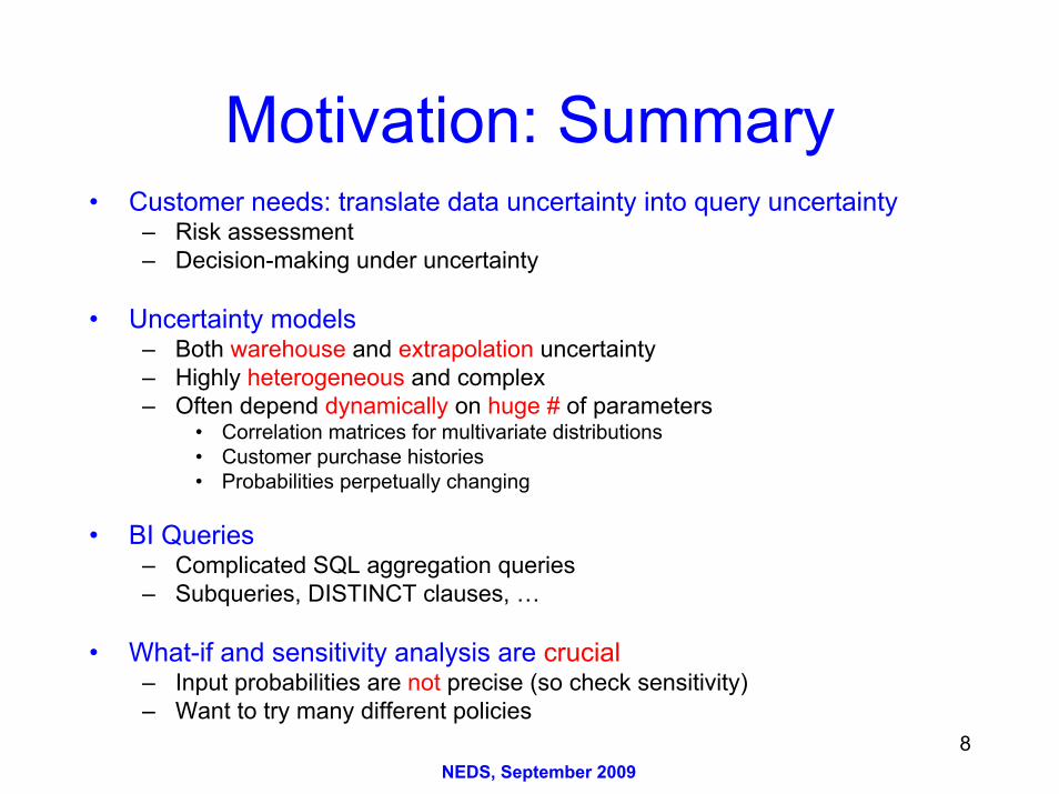
• Drawbacks– Hard-wired uncertainty model– Hard to fit data into tuples– Hard to change probabilities– What-if analysis is hard– Exact analysis (PTIME) only for very
simple queries, data, output stats– Exact methods have trouble with
aggregation queries
10NEDS, September 2009
Outline
• Motivation • MCDB: Monte Carlo Database System• MC3
• Related projects• Future directions
11NEDS, September 2009
The MCDB System
Q(D) = Select SUM(sales)
AS t_salesSchema
VG FunctionsParameter
Tables
Random DB = D
Monte CarloGenerator
d1
d2
:dn
Estimator
i.i.d. samples from possible-worlds
dist’n
E [ t_sales ]Var [ t_sales ]q.01 [ t_sales ]
HistogramError bounds
Inference
ˆˆ
ˆQ(d1)Q(d2)
:Q(dn)
i.i.d. samples from query-result
dist’n
12NEDS, September 2009
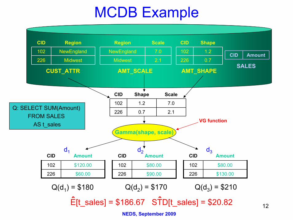
MCDB Example
Q: SELECT SUM(Amount) FROM SALES
AS t_sales
CID Region
102 NewEngland
226 Midwest
CUST_ATTR
CID Shape
102 1.2
226 0.7
AMT_SHAPE
Region Scale
NewEngland 7.0
Midwest 2.1
AMT_SCALE
CID Amount
102 $120.00
226 $60.00
Gamma(shape, scale)
CID Amount
CID Shape Scale
102 1.2 7.0
2.1226 0.7
SALES
CID Amount
102 $80.00
226 $90.00
CID Amount
102 $80.00
226 $130.00
d1 d2
VG function
d3
Q(d1) = $180 Q(d2) = $170 Q(d3) = $210
E[t_sales] = $186.67 STD[t_sales] = $20.82ˆ ˆ
13NEDS, September 2009
Advantages of MCDB
• Flexible and extensible uncertainty model– Can capture extended relational models (Trio, MayBMS, Mystiq,…)– Can capture arbitrarily complex correlations, continuous data– Can capture dynamic, highly parameterized distributions– Can bring complex stochastic models to data (no extraction needed)
• Encapsulates complexity– Once expert has written VG function, naïve user can run queries
• Can handle arbitrary SQL queries
• What-if analysis, sensitivity analysis, data updates are easy
14NEDS, September 2009
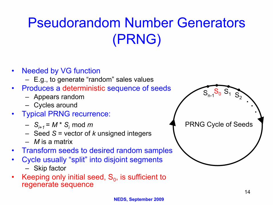
Pseudorandom Number Generators (PRNG)
• Needed by VG function– E.g., to generate “random” sales values
• Produces a deterministic sequence of seeds– Appears random– Cycles around
• Typical PRNG recurrence:– Si+1 = M * Si mod m– Seed S = vector of k unsigned integers– M is a matrix
• Transform seeds to desired random samples• Cycle usually “split” into disjoint segments
– Skip factor• Keeping only initial seed, S0, is sufficient to
regenerate sequence
Sn-1S0 S2
S1
PRNG Cycle of Seeds
. ..
15NEDS, September 2009
VG FunctionsValue WeightSan Jose 0.66
San Francisco 0.34 DiscreteChoice()parameter table
Pseudorandom #seed
• Used to generate instances of values in random tables– Parameter tables are standard relational tables (can index, etc.)– Library of standard functions: DiscreteChoice, Normal, Poisson, …– Can define custom functions (similar to UDFs)
ValueSan Jose
output table(instance)
16NEDS, September 2009
VG Functions and Correlation
ID1 ID2 Cov1
1
2
1 1.23
2 0.17
2 2.45
MDNormal()
Pseudorandom #seed
ID Mean1
2
3.68
4.75
V1 V21.21 2.13
ID Val1
2
1.21
2.13
or
Correlatedcolumns
Correlatedrows
17NEDS, September 2009
Schema Syntax: ExampleCREATE TABLE RAND_CUST (CID, GENDER, MONEY, LIVES_IN) ASFOR EACH d in CUSTWITH MONEY AS Gamma((SELECT n.SHAPE FROM MONEY_SHAPE n WHERE n.CID = d.CID),(SELECT sc.SCALE FROM MONEY_SCALE sc WHERE sc.REGION =
d.REGION),(SELECT SHIFT FROM MONEY_SHIFT))WITH LIVES_IN AS DiscreteChoice ((SELECT c.NAME, c.PROBFROM CITIES cWHERE c.REGION = d.REGION)
)SELECT d.CID, d.GENDER, m.VALUE, l.VALUEFROM MONEY m, LIVES_IN l
18NEDS, September 2009
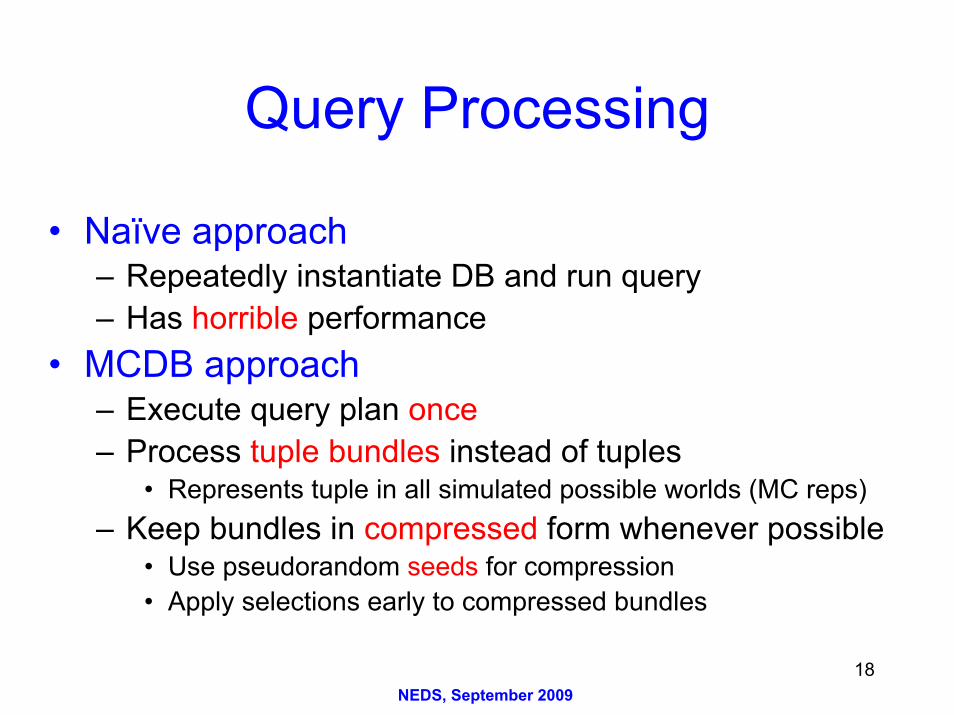
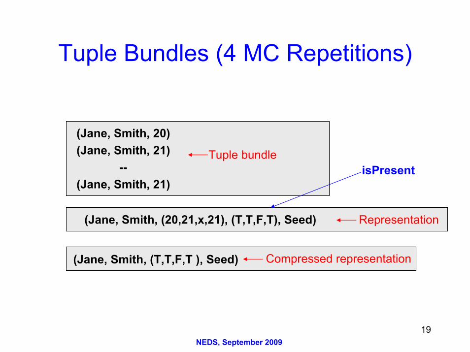
Query Processing
• Naïve approach– Repeatedly instantiate DB and run query– Has horrible performance
• MCDB approach– Execute query plan once– Process tuple bundles instead of tuples
• Represents tuple in all simulated possible worlds (MC reps)– Keep bundles in compressed form whenever possible
• Use pseudorandom seeds for compression• Apply selections early to compressed bundles
FROM OutputTable)SELECT Mu AS Mean, SQRT(Var) AS Stdev,
1.96*SQRT(Var)/SQRT(1000) AS CIHWFROM Stats
Distincttuple values
Frac. replications where
value appears(vs bit vector)
WITH CumDistFn(TotSales, Cum, PrevCum) AS (SELECT TotSales,
SUM(Frac) OVER (ORDER BY TotSalesROWS BETWEEN UNBOUNDED PRECEDING AND CURRENT ROW),
SUM(Frac) OVER (ORDER BY TotSalesROWS BETWEEN UNBOUNDED PRECEDING AND 1 PRECEDING)
FROM OutputTable)SELECT Val FROM CumDistFnWHERE Cum >= 0.5 AND PrevCum < 0.5SQL queries
23NEDS, September 2009
Experimental Queries
• Q1: Next year’s revenue gain from Japanese products– Assuming current trends hold– Each order duplicated Poisson # of times– Poisson mean = (this year)/(last year) for customer
• Q2: Order Delays– From placement to delivery– Fitted Gamma distribution for each delay type (for each part)
• Q3: What if we had used cheapest supplier?– TPC-H only has current prices– Prior prices generated by backwards random walk with drift
• Q4: Change in profits with 5% price increase– Bayesian model of customer demand– Based on all customers orders at current price
• Exploit massive parallelism of MCDB computations– Extend domain of applicability
• Faster path to market?– Forward-looking architecture
• Handle semi-structured, nested data– E.g., web-click example: Petabytes of log file data
• Local expertise/interest in map-reduce– Learning experience for interesting analytical problem– MCDB computations often CPU-intensive– Ease of prototyping
28NEDS, September 2009
Technical Issues
• How to represent bundles?• How to specify map-reduce jobs?• How to parallelize?• How to seed tuple bundles?
• Inter-tuple parallelism– Partition tuple bundles among nodes– Natural fit with Map-Reduce– Good when many bundles or cheap VG functions
• Intra-tuple parallelism– Split up tuple bundles
• Break Monte Carlo replications into chunks– Apply inter-tuple parallelism methods to chunks– Good when few tuples with
• Expensive VG functions and/or• Many MC replications
Tuple 1: (r1,…,r1000)
Tuple 2: (r1,…,r1000)…
Tuple 1: (r1,…,r500)
Tuple 1: (r501,…,r1000)
…
Tuple 2: (r1,…,r500)
Tuple 2: (r501,…,r1000)
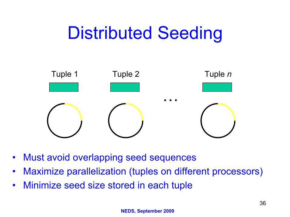
36NEDS, September 2009
Distributed Seeding
• Must avoid overlapping seed sequences• Maximize parallelization (tuples on different processors)• Minimize seed size stored in each tuple
…Tuple 1 Tuple 2 Tuple n
37NEDS, September 2009
Skip-Ahead Method• Well512a generator: period = 2512
• Assume inter-tuple parallelism (for simplicity)• Assume that we know (or have good upper bound for)
– # of bundles seeded per node (= b)– # of seeds per VG function call (= c)– # MC reps (= n)
Tuple j at node i:
Tuple j at node i: Makem = b × i + j
skips of length c × nto get to starting point
{cid: 102, shape: 1.2, scale: 7.0}
{cid: 102, shape: 1.2, scale: 7.0, seed: [i, j] }Actually, only O(log m)
skips needed:pre-computeSkip factors
Seeding
Instantiation
38NEDS, September 2009
Multi-PRNG Method• When # of seeds per VG function call is unknown• When skip-ahead for huge PRNG is hard to implement• Collisions possible, but probability < 10-17
Seeding at node i Instantiation of tuple j
G1
G2
bundle j
bundle j
G3
G4
16 ints
4 ints
6 ints
(small)
s0
(huge)
Shared by All nodes
6 ints x [# bundlesat nodes 0 to (i-1)]
(medium)
(medium)
39NEDS, September 2009
Scale-up Results:Inter-Tuple Parallelism
• Implemented two nontrivial queries from MCDB paper– Jaql: Map-Reduce plan = original MCDB plan– Good scalability with inter-tuple parallelism
0 1 2 3 4 5 6 7 8 9 10600
850
1100
1350
1600
1850
Number of Servers
Run
ning
Tim
e (s
)
Q4Q1
40NEDS, September 2009
Speed-up Results:Intra-Tuple Parallelism
• Implemented two call-option queries (Euro and Asian)– Euro option: expensive VG function, good speed-up– Asian option: cheap VG function, speed-up curve flattens
• Sequential merging of chunks starts to dominate– Moral: choose appropriate parallelization scheme
0 4 8 16 24 32 40 48 56 64 72 80048
16
24
32
40
48
56
64
72
80
Number of Cores
Spe
edup
Ideal SpeedupEuropean OptionAsian Option
41NEDS, September 2009
Outline
• Motivation• MCDB• MC3
• Related projects• Future directions
42NEDS, September 2009
Related Projects• RAQA: Resolution-aware query
answering for Business Intelligence[Sismanis et al., ICDE09]
– Uncertainty due to entity resolution– OLAP querying (roll-up, drill-down)– Bounds on query answers– Implemented via SQL queries– Conservative approach
• ProbIE: Probabilistic info extraction[Michelakis et al., SIGMOD09]
– For rule-based IE system (e.g., SystemT)– Provides confidence #’s for base/derived
annotations– Based on “rule history”, lower-level results– MaxEnt-based learning approach
City State Strict range Status
San Francisco CA [$30,$230] guaranteed
San Jose CA [$70,$200] non-guaranteed
State Strict range Status
CA [$230,$230] guaranteed
Sum(Sales) group by City,State
Sum(Sales) group by State
Annotator rulesLabeled training dataRule features
probIE
Annotation probability
Statisticalmodel
Text
Annotator
Annotation +Rule history
Learning phase
Deploymentphase
43NEDS, September 2009
Outline
• Motivation• MCDB• MC3
• Related projects• Future directions
44NEDS, September 2009
An End-to-End ERP Scenario
Requirements formechanics and parts
(safety margin)
Automobile problem reports (text)
My S-Class slipped out of gear …
ProbIE
My S-Class slipped out of gear …
Tire Problem (0.2)
Transmission problem (0.9)
ProbabilisticBI querying
SELECT COUNT(REPORTS)
WHERE P_TYPE = ‘transmission’
45NEDS, September 2009
Future Directions• Performance
– Query optimizer• E.g., push down inference & instantiation,
• Can analyze arbitrary dynamic customer segments when determining effect of changing EBay pages
Click data for allEBay customers
Global Markov modeldistribution (Dirichelet prior)
Data for onecustomer
Individual Markov modeldistribution (posterior)
x32
p1
p4
p3
p2
x13
x14x34
x24
y32
p1
p4
p3
p2
y13
y14y34
y24
50NEDS, September 2009
Logistics Under Uncertainty• Retailer: ship from warehouses to outlets today or tomorrow?• Deterministic tables
• Random tables
• Queries:
• Issues:– Complicated statistical models for purchase quantity (how to integrate in DB?)– Uncertainty (random tables) depend dynamically on huge number of parameters
• Probabilities sum to 1 in each region– MONEY_SHIFT (SHIFT)– MONEY_SCALE (REGION, SCALE)– MONEY_SHAPE (CID, SHAPE)
Normalizedstorage
1 row, 1 column
53NEDS, September 2009
Schema Syntax: Example 2
CREATE TABLE RAND_CUST (CID, GENDER, MONEY, LIVES_IN) ASFOR EACH d in CUSTWITH MLI AS MyJointDistribution(…)SELECT d.CID, d.GENDER, MLI.V1, MLI.V2FROM MLI
MLI has 1 row, 2 columns
• Suppose MONEY and LIVES_IN are correlated
54NEDS, September 2009
Schema Syntax: Example 3• Correlated sensors
– Sensors in same “sensor group” are correlated (multivariate normal)• Parameter table schemas
– S_PARAMS (ID, LAT, LONG, GID)– MEANS (ID, MEAN)– COVARS (ID1, ID2, COV)
CREATE TABLE SENSORS (ID, LAT, LONG, TEMP) ASFOR EACH g in (SELECT DISTINCT GID FROM S_PARAMS)WITH TEMP AS MDNormal (
(SELECT m.ID, m.MEAN FROM MEANS m S_PARAMS ssWHERE m.ID = ss.ID AND ss.GID = g.GID),(SELECT c.ID1, c.ID2, c.COV FROM COVARS c, S_PARAMS ssWHERE c.ID1 = ss.ID AND ss.GID = g.GID)
)SELECT s.ID, s.LAT, s.LONG, t.VALUEFROM S_PARAMS s, TEMP t WHERE s.ID = t.ID
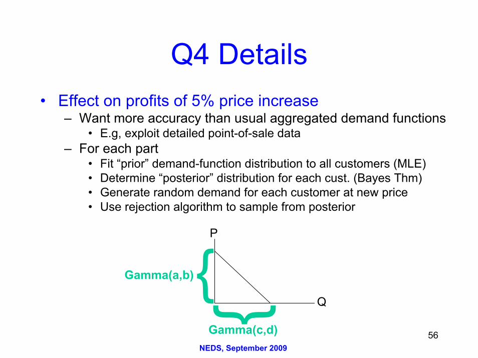
Q4 Details• Effect on profits of 5% price increase
– Want more accuracy than usual aggregated demand functions• E.g, exploit detailed point-of-sale data
– For each part• Fit “prior” demand-function distribution to all customers (MLE)• Determine “posterior” distribution for each cust. (Bayes Thm)• Generate random demand for each customer at new price• Use rejection algorithm to sample from posterior
P
Q{Gamma(a,b)
Gamma(c,d)
57NEDS, September 2009
Nested-Data Experiments
• TPC-H schema is used• Two different ways to nest data
– Nest lineitem table under orders table– Nest lineitem table under partsupp table
• Modified version of Q4 from MCDB paper– Compare MC3 execution time to flat scheme– First nesting scheme: running time is slower– Second nesting scheme: running time is faster
• Only uncertain “leaf attributes” are supported
58NEDS, September 2009
Probabilistic Information Extraction in a Rule-Based System
PP1: <Person><“can be reached at”><PhoneNumber>PP2: <“call”><Person><0-2 tokens><PhoneNumber>PP3: [<Person><PhoneNumber>]sentence
+ Consolidation ruleConsolidate(“Joe Smith”, “Mr. Joe Smith”) = “Mr. Joe Smith”
Derivedannotator
Baseannotator
Baseannotator
Motivation: System T Hand-crafted rules for specific domain:
59NEDS, September 2009
Annotations
Goal: Attach probabilities to annotations in a principled, scalable manner
60NEDS, September 2009
Quantifying this uncertainty is critical as
• Extracted facts can then be queried using probabilistic databases
• Confidence numbers can be used by information integration and search applications
• It helps in improving the recall of annotators!!
61NEDS, September 2009
Our approach
• Propose a probabilistic framework for handling uncertainty in rule-based IE– Each annotation is associated with a confidence
• the probability that the annotation is correct– Probability is obtained by augmenting each annotator with
a statistical model• Design considerations
– Applicable to grammar and declarative rule-based IE systems
– Scale to annotators with a large number of (correlated) rules
– Support incremental improvements in accuracy of probability estimates
• as rules, data, or constraints are added
62NEDS, September 2009
Rule Histories and Features
Please call Heather Choate at
span
P1 P2 P3r = ( 0, 1 , 1)
P1: <Salutation><CapitalizedWord><CapitalizedWord> P2: <First Name Dictionary><Last Name Dictionary>P3: <CapitalizedWord><CapitalizedWord>
Rule history
• Rule features– Qualitative correlations and anti-correlations– Ex: “Rules P1 and P2 tend to occur together”
• Rule history
63NEDS, September 2009
ProbIE Framework(Base Annotator)
Annotator rulesLabeled training data
Rule featuresprobIE
Annotation probability
Statisticalmodel
Text AnnotatorConsolidated span +
Rule history
Learning phase
Extraction (deployment) phase
64NEDS, September 2009
Probability Model of Uncertainty• Binary random variables associated with text and annotator
– A(s) = 1 iff span s is actually a Person– K(s) = 1 iff span s is annotated as a Person by consolidator– R(s) = (R1(s),R2(s),…,Rk(s)) is stochastic rule history on span s
• Ri(s) = 1 iff ith rule holds at least once on span s
• Annotation probability:
q(r) = P(A(s) = 1 | R(s) = r, K(s) = 1)
• Indirect approach (estimate a prob dist’n rather than many small probs)– Estimate
p0(r) = P(R(s) = r | A(s) = 0, K(s) = 1)
p1(r) = P(R(s) = r | A(s) = 1, K(s) = 1) u
= P(A(s) = 1 | K(s) = 1)
– is easy to estimate empirically– Serious data-sparsity problem for p0 and p1: 2k possible histories, little training data– Solution: Fit a parametric model
1
1 0
p (r)q(r)p (r) (1 )p (r)
π=π + − π
65NEDS, September 2009
A Parametric Model• Parametric exponential model for p1 (model for p0 is similar):
– Recall: p1(r) = P(R(s) = r | A(s) = 1, K(s) = 1) with R(s) = (R1(s),…,Rk(s))– From features to constraints
where constants a3, a2,7, etc. computed from training data– Approximate p1 by “simplest” (maximum entropy) distribution satisfying constraints– Equivalent to maximum-likelihood fit of parameter vector for exponential distribution
– Use improved iterative scaling (IIS) to fit from training data
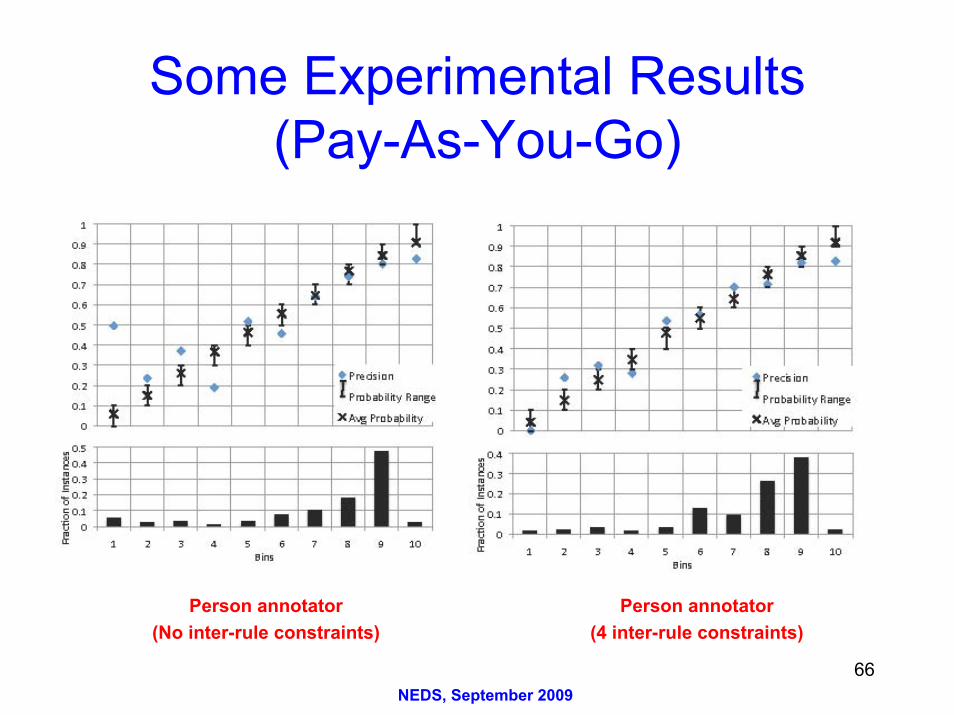
• Model-decomposition methods for IIS scalability to many rules and constraints
• Augment training data to handle constraints with 0 right-hand side
• Methodology extends to derived annotators such as PersonPhone


![DeepSqueeze: Deep Semantic Compression for Tabular Datacs.brown.edu/people/acrotty/pubs/3318464.3389734.pdfdata, columnar compression techniques [12] (e.g., dictionary encoding, run-length](https://static.documents.pub/doc/80x56/5fe6894069cde76c8771dfa5/deepsqueeze-deep-semantic-compression-for-tabular-data-columnar-compression-techniques.jpg)


