5. DETERMINATION OF THE RELATIONSHIPS OF ELECTRICAL RESISTIVITY, SOUND VELOCITY, AND DENSITY/POROSITY OF SEDIMENT AND ROCK BY LABORATORY TECHNIQUES AND WELL LOGS FROM DEEP SEA DRILLING PROJECT SITES 415 AND 416 OFF THE COAST OF MOROCCO Robert E. Boyce, Deep Sea Drilling Project, Scripps Institution of Oceanography, La Jolla, California ABSTRACT Comparisons of compressional-sound velocity and its relationship to wet-bulk density from well-log data with those of laboratory data, from depths of 113 meters to 273 meters below sea floor in Miocene nannofossil marl and chalk, indicate that the porosities of laboratory samples are about 5 porosity units greater than those of in situ sediments (or on the logs). This is in agreement with predictions by Hamilton (1976) for porosity rebound with the release of overburden pressure. The electrical-resistivity relationship with porosity agrees well with the Archie (1942) type relationship. The models, in decreas- ing order of agreement are: Boyce (1968), Archie (1942), Kermabon et al. (1969), Winsauer et al. (1952), and Maxwell (1904). In general, acoustic anisotropy increases with age and depth. Anisotropy is typically 0 to 5 per cent (maximum of 14%) faster parallel to bedding in Tertiary sediments, from 0 to 661 meters below the sea floor, and typically 0 to 30 per cent in mainly Mesozoic sedimentary rock, from 661 to 1624 meters. Acoustic anisotropy is particularly significant (0.4 km/s or greater) when velocities are from 2.0 to 4.2 km/s. INTRODUCTION This paper is concerned with the physical-property relationships enumerated below, using samples and well logs from Sites 415 and 416, off the coast of Morocco (Figure 1): 1. We will study the electrical formation factor and porosity relationships for soft sediments. These are sparse- ly reported in the literature yet are essential to the prop- er interpretation of electric logs; 2. We will undertake one of the first systematic studies of acoustic anisotropy for terrigenous sediments and rocks and its relationship to density and porosity. This information is valuable for the correct interpreta- tion of gravity, seismic-reflection and -refraction, and Sonobuoy data; 3. We will test the theory that in situ porosities, for uncemented sediments with significant overburden pres- sure, are lower than those determined in the laboratory without overburden pressure. This is important where laboratory density and porosity values are used as in- dexes to other in situ physical properties, sedimentation rates, etc.; and 4. We will also attempt to calculate in situ interval velocities of the geologic section penetrated at Sites 415 and 416. These values are needed when attempting to correlate the stratigraphic data obtained from the drill holes with seismic profiles. The comparison of laboratory-measured compres- sional-sound velocity and wet-bulk density with the ve- locity and density measured in situ from the Schlumber- ger well logs (see site chapters, this volume) will only be for Hole 415, as this hole provided the only successful density-log data on Leg 50. The data are from Miocene hemipelagic nannofossil marl and chalk, from depths of 113 meters and 273 meters below the sea floor. The main purpose of this study is to examine the porosity in- crease or rebound as sedimentary samples are released from the overburden pressure (weight, in sea water, of overlying sediment grains). Porosity rebound has been predicted through laboratory consolidation studies by Laughton (1957) and Hamilton (1959, 1964, 1965, 1976). The data from Leg 50 now offer the opportunity to test these predictions by comparing in situ logging measurements of density and velocity with laboratory measurements. The relationship of the electrical formation factor (ratio of the electrical resistivity of the sediment to that of the interstitial water) to porosity is significant in the interpretation of the electric well logs in terms of poros- ity; its investigation is all the more important because only a few published studies of modern marine sedi- ments exist (Boyce, 1968; Kermabon et al., 1969). If the porosities derived from the density and electric logs do not correspond, within the limits of experimental error, the following causes (singly or in combination) are indi- cated: (1) conductive metallic minerals, (2) anomalies in the salinities of interstitial water, (3) an anomalous tem- perature, and (4) a large amount of minerals with very high or low grain density. 305
Transcript
5. DETERMINATION OF THE RELATIONSHIPS OF ELECTRICAL RESISTIVITY,SOUND VELOCITY, AND DENSITY/POROSITY OF SEDIMENT AND ROCK
BY LABORATORY TECHNIQUES AND WELL LOGS FROM DEEP SEA DRILLING PROJECTSITES 415 AND 416 OFF THE COAST OF MOROCCO
Robert E. Boyce, Deep Sea Drilling Project, Scripps Institution of Oceanography, La Jolla, California
ABSTRACT
Comparisons of compressional-sound velocity and its relationshipto wet-bulk density from well-log data with those of laboratory data,from depths of 113 meters to 273 meters below sea floor in Miocenenannofossil marl and chalk, indicate that the porosities of laboratorysamples are about 5 porosity units greater than those of in situsediments (or on the logs). This is in agreement with predictions byHamilton (1976) for porosity rebound with the release of overburdenpressure. The electrical-resistivity relationship with porosity agreeswell with the Archie (1942) type relationship. The models, in decreas-ing order of agreement are: Boyce (1968), Archie (1942), Kermabonet al. (1969), Winsauer et al. (1952), and Maxwell (1904). In general,acoustic anisotropy increases with age and depth. Anisotropy istypically 0 to 5 per cent (maximum of 14%) faster parallel to beddingin Tertiary sediments, from 0 to 661 meters below the sea floor, andtypically 0 to 30 per cent in mainly Mesozoic sedimentary rock, from661 to 1624 meters. Acoustic anisotropy is particularly significant(0.4 km/s or greater) when velocities are from 2.0 to 4.2 km/s.
INTRODUCTION
This paper is concerned with the physical-propertyrelationships enumerated below, using samples and welllogs from Sites 415 and 416, off the coast of Morocco(Figure 1):
1. We will study the electrical formation factor andporosity relationships for soft sediments. These are sparse-ly reported in the literature yet are essential to the prop-er interpretation of electric logs;
2. We will undertake one of the first systematicstudies of acoustic anisotropy for terrigenous sedimentsand rocks and its relationship to density and porosity.This information is valuable for the correct interpreta-tion of gravity, seismic-reflection and -refraction, andSonobuoy data;
3. We will test the theory that in situ porosities, foruncemented sediments with significant overburden pres-sure, are lower than those determined in the laboratorywithout overburden pressure. This is important wherelaboratory density and porosity values are used as in-dexes to other in situ physical properties, sedimentationrates, etc.; and
4. We will also attempt to calculate in situ intervalvelocities of the geologic section penetrated at Sites 415and 416. These values are needed when attempting tocorrelate the stratigraphic data obtained from the drillholes with seismic profiles.
The comparison of laboratory-measured compres-sional-sound velocity and wet-bulk density with the ve-
locity and density measured in situ from the Schlumber-ger well logs (see site chapters, this volume) will only befor Hole 415, as this hole provided the only successfuldensity-log data on Leg 50. The data are from Miocenehemipelagic nannofossil marl and chalk, from depths of113 meters and 273 meters below the sea floor. Themain purpose of this study is to examine the porosity in-crease or rebound as sedimentary samples are releasedfrom the overburden pressure (weight, in sea water, ofoverlying sediment grains). Porosity rebound has beenpredicted through laboratory consolidation studies byLaughton (1957) and Hamilton (1959, 1964, 1965,1976). The data from Leg 50 now offer the opportunityto test these predictions by comparing in situ loggingmeasurements of density and velocity with laboratorymeasurements.
The relationship of the electrical formation factor(ratio of the electrical resistivity of the sediment to thatof the interstitial water) to porosity is significant in theinterpretation of the electric well logs in terms of poros-ity; its investigation is all the more important becauseonly a few published studies of modern marine sedi-ments exist (Boyce, 1968; Kermabon et al., 1969). If theporosities derived from the density and electric logs donot correspond, within the limits of experimental error,the following causes (singly or in combination) are indi-cated: (1) conductive metallic minerals, (2) anomalies inthe salinities of interstitial water, (3) an anomalous tem-perature, and (4) a large amount of minerals with veryhigh or low grain density.
305
R. E. BOYCE
40°N
AFRICA
Agadir SubmarineCanyon
500 Kmat lat. 20°N
30°W 25° 20° 15° 10° 5°
Figure 1. Index map showing locations of DSDP Sites 370, 415, and 416.
The oil companies have mainly studied formationfactor-porosity relationships of consolidated sedimentsor rock, and their empirical formulas (Winsauer et al.,1952; and others) may therefore not be directly appli-cable to soft, deep-sea sediments. Archie (1942) devel-oped an equation applicable to "clean" sandstone (wellsorted, without clay), but it may not accurately predictporosities for sediment incorporating a major fractionof clay-type minerals such as occur in the Leg 50 hemi-pelagic sediments.
Maxwell's (1904) equation constitutes a theoreticalapproach for spheres in suspension, which should pro-vide a lower limit of porosity. However, most sedimentsor rocks are not accurately represented by such a simplemodel, since they generally have irregularly shapedgrains. Conducting ions must therefore travel a longeraverage path and so will have a greater resistivity andformation factor than those derived from the Maxwellequation for spherical particles.
DATA, DEFINITIONS, AND METHODSThe sediment classification is discussed in the Ex-
planatory Notes (this volume). Wet-bulk density isdefined as the ratio of weight of the water-saturated sed-iment or rock sample to its volume, expressed asg/cm3.Water content is the ratio of the weight of seawater in the sample to the weight of the saturated sam-ple, and is expressed as a percentage. Porosity is theratio of the pore volume in a sample to the volume ofthe saturated sample, and is also expressed as a percen-tage. Acoustic impedance is defined as the product ofthe velocity and wet-bulk density, and is expressed as(g 105)/(cm2-s). All the equations, derivations, andtechniques are discussed in detail in Boyce (thisvolume).
With respect to sampling, we generally waited at least4 hours after the core was brought on deck to allow it to
reach room temperature. We then cut and removed anundisturbed (visible, undistorted bedding), water-satu-rated, compressional-sound-velocity sample, about 2.5cm thick. The sample was carefully smoothed with asharp knife or file. Velocities were measured to within±2 per cent accuracy with the Hamilton Frame veloc-imeter (Boyce, 1976a, and this volume), perpendicularand parallel to bedding. Immediately afterward, its wet-bulk density was measured to within ±2 or 3 per centprecision with the Gamma Ray Attenuation PorosityEvaluator (GRAPE) (Evans, 1965) as modified in Boyce(1976a, and this volume), using special 2-minute gam-ma-ray counts. Then, the wet-water content of a sub-sample was determined by weighing the sample both wetand after drying 24 hours at 110 °C. The weight of evap-orated water was corrected for salt (45%0) to give theweight of sea water (Boyce, 1976a, and this volume;Hamilton, 1971). The estimated precision is ±2.5 percent (absolute). Porosity (precision of ±6%) is deter-mined from the product of the wet-water content andwet-bulk density, divided by the density of the intersti-tial water (1.032 g/cm3). The acoustic impedance is ob-tained from the product of the vertical velocity and thewet-bulk density. The laboratory results have been tabu-lated in the site chapters (this volume).
In situ sound velocity and wet-bulk density wereobtained from the Schlumberger Ltd. well logs: Forma-tion Compensated Density (FDC), Bore Hole Compen-sated Sonic (BHC), and Dual Induction-Laterolog-8(DIL). They are discussed in Appendix II (Boyce, thisvolume) and the well-log data in analog form are pre-sented in the site chapters (this volume).
Electrical Resistivity
The electrical resistivity of any material is defined asthe resistance, in ohms, between opposite faces of a unitcube of that material. If the resistance of a conducting
306
PHYSICAL PROPERTIES AND WELL LOGS
cube with a length L and cross-sectional area A is r, thenthe resistivity Ro is
= rA/L = ohm-m (1)
Electrical conduction through saturated sediment iscomplicated by a framework that generally consists ofnonconducting mineral grains. If the sediment consistsof nonconducting minerals, the electrical conduction isprimarily through the interstitial water, whose conduc-tivity varies with temperature, pressure, and salinity(Home, 1965; Home and Courant, 1964; Home andFry singer, 1963; Thomas et al., 1934). However, con-duction through the fluid can be modified significantlyif metallic minerals are present with appreciable conduc-tivity, or clay-type minerals that exchange or withdrawions from the interstitial water (de Witte, 1950a,b; Pat-node and Wyllie, 1950; Keller, 1951; Berg, 1952; Win-sauer and McCardell, 1953; Wyllie, 1955). Charged col-loidal particles and exchanged ions are not necessarilyremoved from the sediment when the interstitial water issampled; therefore, they do not contribute to what isnormally thought of as the water salinity (Keller, 1951;Howell, 1953).
The formation factor, F, is the ratio of electricalresistivity of the saturated sediment, Ro, to the resistivi-ty of the interstitial water, Rw, at the same temperatureand pressure (Archie, 1942):
F = Ro
/R
w (2)
The formation factor has been related to porosity andfluid salinity of rocks or sediments by Archie (1942,1947), Winsauer et al. (1952), and others (Table 1).Where the mineral composition of the sediment forms anonconductive matrix and the interstitial water conduc-tivity is high, /MS considered to be the "true" formationfactor, which, with increasing salinity of the interstitialwater, approaches a constant value for a given porosityand rock sample (Patnode and Wyllie, 1950; Keller andFrischkecht, 1966).
Where, on the other hand, sediments contain miner-als that are conductors, this ratio is considered to be an"apparent" formation factor, and is lower than the"true" formation factor of sediments, for a given set ofporosity, textural, and cementation characteristics. The"apparent" formation factor approaches a constantvalue with different salinities, at a given porosity, onlyif the conductivity of the interstitial water is muchgreater than that of the conducting minerals (Berg,1952; Howell, 1953; Wyllie and Southwick, 1954;Wyllie, 1955).
The variation of apparent formation factor withinterstitial-water resistivity may be in part related to thedistribution of conducting grains in a sample. Wyllieand Southwick (1954) developed a model showing thatthe connected conducting grains are conductors in par-allel and isolated conducting grains are conductors inseries with the interstitial fluid. If the interstitial fluid isa good conductor, all the conducting grains contributeto the overall conduction of the rock matrix. If the in-
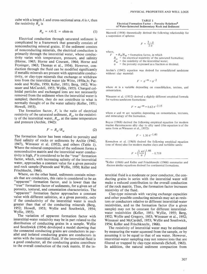
Maxwell (1904) theoretically derived the following relationship fora suspension of spheres:
F =3 -
where,F - Ro/Rw = formation factor, in which
Ro = the electrical resistivity of the saturated formation;Rw - the resistivity of the interstitial water;Φ - the porosity expressed as a fraction or decimal.
Archie's (1942) equation was derived for consolidated sandstonewithout clay material:
F =
where m is a variable depending on consolidation, texture, andcementation.
Winsauer et al. (1952) derived a slightly different empirical formulafor various sandstone formations:
F = aΦ'm = 0.62é>-2•15
where a and m are variables depending on cementation, textures,and mineralogy of the formation.
Boyce (1968) derived the following empirical equation for modernmarine diatomaceous silty clay to silty sand (this equation is of thesame form as Winsauer et al., 1952):
F = 1.30 θ~ 1 - 4 5
Kermabon et al. (1969) derived the following empirical equation(one of three) also for modern marine clays and turbidite sands:
l 4 51 4 6
-0.719
aKeller (1966) and Keller and Frischknecht (1966) summarize anddiscuss similar equations derived for continental formations.
terstitial fluid is a moderate or poor conductor, the con-ducting grains in series with the interstitial water willmake a reduced contribution to the overall conductionof the rock matrix. Thus, the formation factor increasesresistivity of the fluid.
Clay-type minerals with varying exchange capacitiesand other possible conducting minerals may act as resis-tors or conductors relative to different interstitial-waterresistivities, and so the formation factor (for a givensample) may not be constant for different interstitial-water resistivities (Keller, 1951; Wyllie, 1955; Berg,1952; Wyllie and Gregory, 1953; Winsauer et al., 1952;Winsauer and McCardell, 1953; Wyllie and Southwick,1954; Keller and Frischknecht, 1966).
The resistivity of interstitial water may be estimatedby measuring the water squeezed from the sample, or byassuming it to be equal to that of sea water. However,interstitial-water sampling may not remove ions that arefiltered or trapped by clay-type minerals (Scholl, 1963).In addition, the natural sediment compaction from
307
R. E. BOYCE
overburden pressure may trap or filter various ions asthe fluid migrates. Thus the interstitial fluid may have adifferent chemical composition from that of the originalinterstitial sea water (Siever et al. 1961; Siever et al.,1965). Therefore, the electrical resistivity of the intersti-tial water determined, for example, by using data ofThomas et al. (1934) may be in error, because these in-vestigators assumed a chemical composition like that ofseawater.
Fresh sediment may be anisotropic with respect toelectrical resistivity (Bedcher, 1965), but consolidatedsediments and rock are anisotropic. Resistivity parallelto bedding is typically lower than that perpendicular tobedding (Keller, 1966; Keller and Frischknecht, 1966).
The shapes of the individual mineral grains also playa part: the more angular grains create a greater pathlength through the sediment and thus a higher resistivityand higher formation factor for a given porosity (Wyllieand Gregory, 1953). The resistivity is further affected bygrain-size distribution, particularly for clay-type min-erals. A lesser grain size gives a greater surface area withan ion-exchange capacity and thus increases the numberof ionic-cloud conductors in a given sample. To a lesserextent this is also true of non-clay-type minerals, such asquartz and feldspar (Keller and Frischknecht, 1966).
Sound Velocity
Compressional-sound velocity in isotropic materialhas been defined (Wood, 1941; Bullen, 1947; Birch,1961; Hamilton, 1970) as:
V =1(3)
9b
where V is the compressional velocity,
pb is the wet-bulk density in g/cm3, where9b = Pw<t> + 0 ~Φ) Pg> i n which 0 is thefractional porosity of the sediment orrock and the subscripts b, g, and w, rep-resent the wet-bulk density, grain density,and water density, respectively,
k is the incompressibility or bulk modulus,and
µ is the shear (rigidity) modulus.
Where samples are anisotropic, k and µ may haveunique values for the corresponding vertical and hori-zontal directions. See Laughton (1957) for discussionsof anisotropy.
Compressional velocity of sediments and rocks hasbeen related to the sediment components by Wood(1941), Wyllie et al. (1956), and Nafe and Drake (1957),whose equations are listed in Table 2 and will be dis-cussed later. Velocity is related to mineralogical compo-sition, fluid content, temperature, pressure, grain size,texture, cementation, direction with respect to beddingor foliation, and alteration, as summarized in Press(1966).
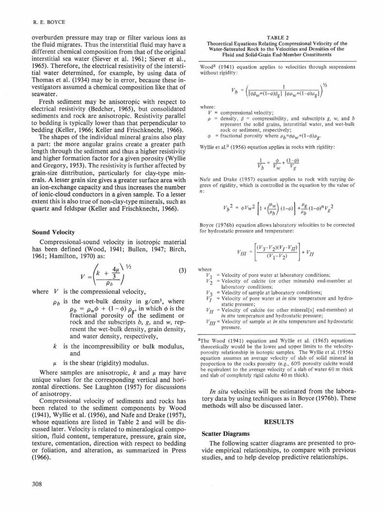
TABLE 2Theoretical Equations Relating Compressional Velocity of theWater-Saturated Rock to the Velocities and Densities of the
Fluid and Solid-Grain End-Member Constituents
Wooda (1941) equation applies to velocities through suspensionswithout rigidity:
Vu =1
3w+(l-Φ)ßg] [ΦPw+(l-Φ)Pg
where:V = compressional velocity;p = density, ß = compressibility, and subscripts g, w, and b
represent the solid grains, interstitial water, and wet-bulkrock or sediment, respectively;
Φ - fractional porosity where pb=Φpw+(l-Φ)p>
Wyllie et al.a (1956) equation applies in rocks with rigidity:
J_= 0 , d-0)
Nafe and Drake (1957) equation applies to rock with varying de-grees of rigidity, which is controlled in the equation by the value of
Vb
2 =
Boyce (1976b) equation allows laboratory velocities to be correctedfor hydrostatic pressure and temperature:
777(V3-V2×VrVff)
+ VII
whereVΛ = Velocity of pore water at laboratory conditions;Vy - Velocity of calcite (or other minerals) end-member at
laboratory conditions;Kj = Velocity of sample at laboratory conditions;Vj = Velocity of pore water at in situ temperature and hydro-
static pressure;VTT = Velocity of calcite (or other mineral [s] end-member) at
in situ temperature and hydrostatic pressure;VTTT = Velocity of sample at in situ temperature and hydrostatic
pressure.
aThe Wood (1941) equation and Wyllie et al. (1965) equationstheoretically would be the lower and upper limits to the velocity-porosity relationship in isotopic samples. The Wyllie et al. (1956)equation assumes an average velocity of slab of solid mineral inproportion to the rocks porosity (e.g., 60% porosity calcite wouldbe equivalent to the average velocity of a slab of water 60 m thickand slab of completely rigid calcite 40 m thick).
In situ velocities will be estimated from the labora-tory data by using techniques as in Boyce (1976b). Thesemethods will also be discussed later.
RESULTS
Scatter Diagrams
The following scatter diagrams are presented to pro-vide empirical relationships, to compare with previousstudies, and to help develop predictive relationships.
308
PHYSICAL PROPERTIES AND WELL LOGS
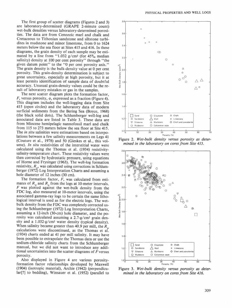
The first group of scatter diagrams (Figures 2 and 3)are laboratory-determined (GRAPE 2-minute count)wet-bulk densities versus laboratory-determined porosi-ties. The data are from Cenozoic marl and chalk andCretaceous to Tithonian sandstone and siltstone turbi-dites in mudstone and minor limestone, from 0 to 1624meters below the sea floor at Sites 415 and 416. In thesediagrams, the grain density of each sample may be esti-mated by a line from "1.032 g/cm3 (for 45%0 mediansalinity) density at 100 per cent porosity" through "thegiven datum point" to the "0 per cent porosity axis."The grain density is the bulk-density value at 0 per centporosity. This grain-density determination is subject togreat uncertainty, especially at high porosity, but it atleast permits identification of sample data of doubtfulaccuracy. Unusual grain-density values could be the re-sult of laboratory mistakes or gas in the samples.
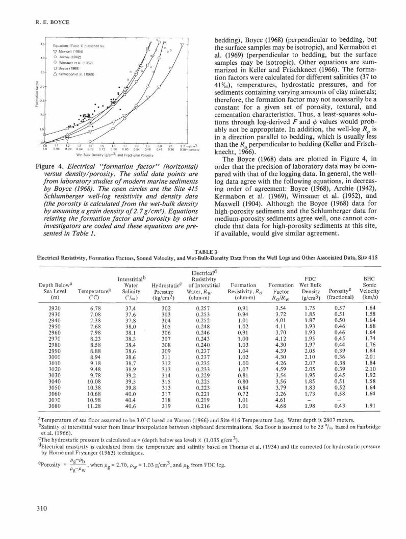
The next scatter diagram plots the formation factor,F, versus porosity, </>, expressed as a fraction (Figure 4).This diagram includes the well-logging data from Site415 (open circles) and the laboratory data of modernsurficial sediments from the Bering Sea (Boyce, 1968)(the black solid dots). The Schlumberger well-log andassociated data are listed in Table 3. These data arefrom Miocene hemipelagic nannofossil marl and chalkfrom 115 to 273 meters below the sea floor at Site 415.The in situ salinities were estimations based on interpo-lations between a few salinity measurements on Legs 41(Couture et al., 1978) and 50 (Gieskes et al., this vol-ume). In situ resistivities of the interstitial water werecalculated using the Thomas et al. (1934) resistivity-salinity-temperature chart. These resistivity values werethen corrected by hydrostatic pressure, using equationsof Home and Frysinger (1963). The well-log formationresistivity, Ro, was calculated using corrections in Schlum-berger (1972) Log Interpretation Charts and assuming ahole diameter of 12 inches (30 cm).
The formation factor, F, was calculated from esti-mates of Rw and Rq from the logs at 10-meter intervals.F was plotted against the wet-bulk density from theFDC log, also measured at 10-meter intervals, using theassociated gamma-ray logs to be certain the same litho-logical interval is used as for the electric logs. The wet-bulk density from the FDC was completely corrected us-ing the Schlumberger (1972) Log Interpretation Charts,assuming a 12-inch (30-cm) hole diameter, and the po-rosity was calculated assuming a 2.7-g/cm3 grain den-sity and a 1.032-g/cm3 water density (typical density).When salinity became greater than 40.9 per mill, the Rcalculations were discontinued, as the Thomas et aL(1934) charts ended at 41 per mill salinity. It may havebeen possible to extrapolate the Thomas data or use thesodium-chloride salinity charts from the Schlumbergermanual, but we did not want to introduce any addi-tional uncertainties into the scatter diagrams of F versusporosity.
Also displayed in Figure 4 are various porosity-formation factor relationships developed by Maxwell(1904) (isotropic material), Archie (1942) (perpendicu-lar[?] to bedding), Winsauer et al. (1952) (parallel to
<x>
o
Δ
o
Δ Δ
Δ°
oV
o
Sand
Sandstone
Siltstone
Mudstone
0
ΔΔ
o
Clayston
Marl
Marlston
Calcareo
e
e
us
O
0
oooze
Chalk
Limesto
Chert ar
ne
d porcelanite
Porosity (%)
Figure 2. Wet-bulk density versus porosity as deter-mined in the laboratory on cores from Site 415.
O
π
D
V
O
Sand
Sandstone
Siltstone
Mudstone
0
ΔΔ
o
Claystone
Marl
Marlstone
Calcareous ooze
O
0
o
Chalk
Limestone
Chert and porcelanite
Porosity
Figure 3. Wet-bulk density versus porosity as deter-mined in the laboratory on cores from Site 416.
309
R. E. BOYCE
Equations (Table 1) published by
V Maxwell (1904)
O Archie (1942)
O Winsaueret al. (1952)
G Boyce (1968)
Δ Kermabon et al. (1969)
0.78 0.72 0.66 0.60 0.54 0.48 0.4?
Wet Bulk Density (g/cm3) and Fractional Porosity
Figure 4. Electrical "formation factor" (horizontal)versus density/porosity. The solid data points arefrom laboratory studies of modern marine sedimentsby Boyce (1968). The open circles are the Site 415Schlumberger well-log resistivity and density data(the porosity is calculated from the wet-bulk densityby assuming a grain density of 2.7 g/cmi). Equationsrelating the formation factor and porosity by otherinvestigators are coded and these equations are pre-sented in Table 1.
bedding), Boyce (1968) (perpendicular to bedding, butthe surface samples may be isotropic), and Kermabon etal. (1969) (perpendicular to bedding, but the surfacesamples may be isotropic). Other equations are sum-marized in Keller and Frischknect (1966). The forma-tion factors were calculated for different salinities (37 to41 ‰), temperatures, hydrostatic pressures, and forsediments containing varying amounts of clay minerals;therefore, the formation factor may not necessarily be aconstant for a given set of porosity, textural, andcementation characteristics. Thus, a least-squares solu-tions through log-derived F and Φ values would prob-ably not be appropriate. In addition, the well-log Ro isin a direction parallel to bedding, which is usually lessthan the Ro perpendicular to bedding (Keller and Frisch-knecht, 1966).
The Boyce (1968) data are plotted in Figure 4, inorder that the precision of laboratory data may be com-pared with that of the logging data. In general, the well-log data agree with the following equations, in decreas-ing order of agreement: Boyce (1968), Archie (1942),Kermabon et al. (1969), Winsauer et al. (1952), andMaxwell (1904). Although the Boyce (1968) data forhigh-porosity sediments and the Schlumberger data formedium-porosity sediments agree well, one cannot con-clude that data for high-porosity sediments at this site,if available, would give similar agreement.
TABLE 3Electrical Resistivity, Formation Factors, Sound Velocity, and Wet-Bulk-Density Data From the Well Logs and Other Associated Data, Site 415
aTemperature of sea floor assumed to be 3.0°C based on Warren (1966) and Site 416 Temperature Log. Water depth is 2807 meters."Salinity of interstitial water from linear interpolation between shipboard determinations. Sea floor is assumed to be 35 %o based on Fairbridge
et al. (1966).cThe hydrostatic pressure is calculated as = (depth below sea level) × (1.035 g/cm3)."Electrical resistivity is calculated from the temperature and salinity based on Thomas et al. (1934) and the corrected for hydrostatic pressureby Home and Frysinger (1963) techniques.
ePorosity = , when p g = 2.70, p w = 1.03 g/cmá, and p b from FDC log.
310
PHYSICAL PROPERTIES AND WELL LOGS
The primary importance of Figure 4 is to demon-strate the relationship of the Schlumberger logging datato various F-<f> equations, so that the latter may be usedin determining the porosity from the electric-log data,and in estimating the accuracy of the results.
Figure 5 displays the formation factor versus velocityfrom the Schlumberger logs from Sites 415 and 416, forCenozoic hemipelagic nannofossil marl and chalk from100 to 450 meters below the sea floor at Sites 415 and416. There is no precise relationship for these high-porosity sediments in which the sound velocity does notvary greatly with porosity, but F does have a distinctrelationship to porosity. In addition, Ro is parallel tobedding, which is usually less than Ro normal to bed-ding (Keller and Frischknecht, 1966), while the velocityis perpendicular to bedding, which is normally less thanthat parallel to the bedding. (See Table 3 and 4.)
Acoustic anisotropy is important for estimating ver-tical velocities (for seismic-reflection profiles) from thehorizontal velocities determined by refraction techniques,and the oblique velocities determined by Sonobuoy tech-niques.
Acoustic anisotropy in sedimentary rock may becreated by some combination of the following variablesas summarized in Press (1966): (1) alternating layerswith high- or low-velocity materials; (2) tabular miner-als that are aligned with bedding, thus creating fewergaps in a direction parallel to bedding; (3) the presenceof minerals with acoustic anisotropy, whose high-velocity axis may be aligned with the bedding plane; and(4) foliation parallel to bedding.
Figure 6 shows acoustic anisotropy for Cenozoic hem-ipelagic nannofossil marls and chalk, from 0 to 661 me-ters below the sea floor, and mainly Cretaceous to Tith-onian sandstone and siltstone turbidites in mudstoneand minor limestone from 661 to 1624 meters below thesea floor. In general, the anisotropy is small (0-5% istypical, with a maximum of 15%) for Cenozoic hemipe-lagic sediments with velocities less than about 2 km/s.Acoustic anisotropy of the Cretaceos-Jurassic sedimen-tary rocks, which have velocities between about 2.0 and4.2 km/s, is about 0.4 km/s, more in the horizontalthan in the vertical plane. Some samples have an abso-lute anisotropy as great as 1.0 km/s. The relative acous-tic anisotropy ranges from 0 to 30 per cent, 5 to 20 percent being typical. The mudstones, which have velocitiesof 2.0 to 3.0 km/s, tend to have the greatest anisotropy,as compared with the higher-velocity (3 to 4.2 km/s)sandstones, siltstones, and limestones. Where the sand-stone, siltstone, and limestone have velocities greaterthan about 4.2 km/s, the acoustic anisotropy becomesmuch less significant, as the sample is more thoroughlycemented.
Based on data from the Cenozoic to Tithonian sedi-ments and rocks at Sites 415 and 416, the scatter dia-grams of horizontal and vertical velocity versus wet-theoretical equations (listed in Table 2), which utilizedhere for simplicity a calcium-carbonate matrix (6.45km/s; 2.72 g/cm3) saturated with sea water (1.53 km/s;1.025 g/cm3). Wood's (1941) equation assumes a sus-
6> Δ Δ °o o
o o Q̂ o oo O o o
oΔ Δ ΔA, Δ
Δ Δo
Formation factor
Figure 5. Vertical velocity versus (horizontal) electricalformation factor for Site 415 (triangles) and Site 416(circles) from the well-log data.
ππV
o
.Sand
Sandstone
Siltstone
Mudstone
oΔΔ
o
Claystone
Marl
Marlstone
Calcareous ooze
O
o
o
Chalk
Limestone
Chert andporcelanite
1.5 2.0 3.0 4.0
Horizontal velocity (km/s)
Figure 6. Laboratory horizontal velocity versus labora-tory vertical velocity, which are coded for lithologicaltype. Data are from Sites 415 and 416.
bulk density (Figure 7) and porosity (Figure 8) representone of the first systematic studies of terrigenous sedi-ments to introduce anisotropy into these relationships.The latter are important for the interpretation of gravityand seismic data in terms of subsurface structures andfor well-log analysts who may be required to estimateporosity from a sonic log.
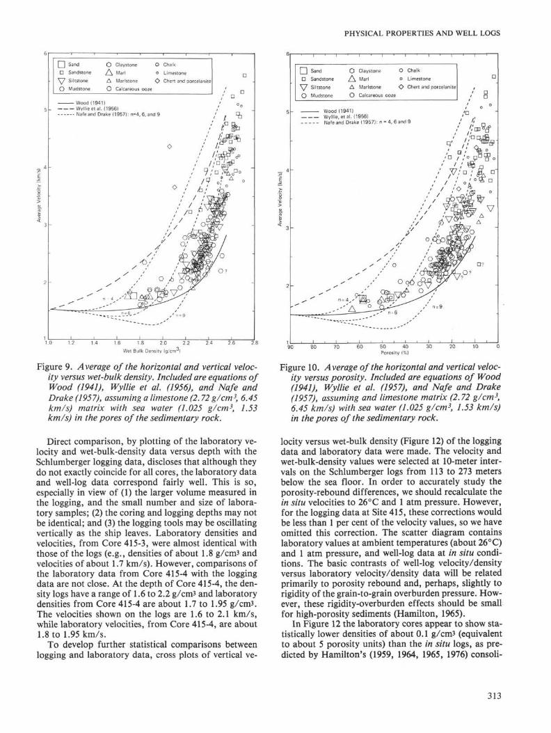
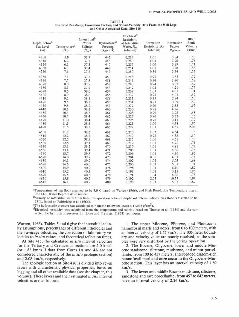
The average of the horizontal and vertical velocity isplotted against wet-bulk density and porosity in Figures9 and 10, respectively. These figures illustrate the Wood(1941), Wyllie et al. (1956), and Nafe and Drake (1957)
311
R. E. BOYCE
Q SandD Sandstone
V Siltstone
O Mudstone
Open Symbols =
Solid Symbols =
0ΔΔ
oHorizo
Claystone
Marl
Marlstone
Calcareous ooze
ital Velocity
Vertical Velocity
O
o
o
Chalk
Limestone
Chert and porcelanite
1.0 1.2 1.6 1.8 2.0 2.2 2.4 2.6 2.8
Wet Bulk Density (g/cm3)
Figure 7. Laboratory horizontal and vertical velocitiesversus laboratory wet-bulk density, from Sites 415and 416.
theoretical equations (listed in Table 2), which utilizehere for simplicity a calcium-carbonate matrix (6.45km/s; 2.72 g/cm3) saturated with sea water (1.53 km/s;1.025 g/cm3). Wood's (1941) equation assumes a sus-pension of spheres without rigidity and theoretically ap-plies best to soft, unconsolidated sediment. This equa-tion would tend to be the lower velocity limit. The Wyl-lie et al. (1956) equation assumes (1) complete rigidity ofthe carbonate matrix and (2) that the model is similar tosound traveling perpendicularly through a solid slab ofcalcite and slab of water. The ratio of the thicknesses ofthe water and the calcite slabs is the same proportion asthe porosity of the sample. This equation should theo-retically be the upper velocity limit. The Nafe and Drakeequation is shown for n values of 4, 6, and 9. No singlevalue of n fits all the data. For some of its values, theNafe and Drake (1957) equation velocities may be toohigh (greater than those from the Wyllie et al. equation),or too low (lower than those from the Wood equation).
Acoustic impedance versus vertical velocity is plottedin Figure 11 for the Cenozoic to Tithonian sedimentsand rocks from Sites 415 and 416 and approximates alinear relationship. Normally the plot segregates differ-ent mineralogies into separate lines representing differ-ent bulk elasticity for rock types such as basalt, elastics,limestone, and chert (Boyce, 1976b). However, in Fig-ure 11, a single line is developed for Leg 50 clastic sedi-
Q SandD Sandstone
V Siltstone
O Mudstone
Open Symbols =
Solid Symbols =
0 Claystone
Δ MarlΔ Marlstone
O Calcareous ooze
Horizontal Velocity
Vertical Velocity
O
o
o
Chalk
Limestone
Chert and porcelanite
80 70 60 50 40 30 20 10 0
Porosity (%)
Figure 8. Laboratory-determined horizontal and verti-cal velocity versus porosity, from Sites 415 and 416.
ments, sedimentary rock, and limestone. Different min-eralogies do not display different lines for carbonatesand terrigenous elastics, as in Boyce (1976b), becausethe quartz-feldspar-clay elastics are cemented by calcite.
Comparison of Laboratory Velocity/Density toIn Situ Velocity/Density
In attempting to calculate in situ velocities from labo-tory velocities, it is important to correct the latter forthe porosity rebound a sample undergoes when it is re-moved from deep within the sea floor, thereby releasingthe overburden pressure (as discussed by Hamilton,1965, 1976). According to Hamilton (1976), it amountsto up to 8 per cent porosity units, depending on thelithology of the laboratory-uncemented sample and onthe depth at which the sample was buried below the seafloor.
Leg 50 laboratory data and well-logging data offer anopportunity to make a very cursory study of this prob-lem, albeit for only a very limited range of conditionsand only at Site 415, which is the only site of Leg 50where the density log was successful. At this site we ob-tained good Schlumberger logs for wet-bulk density andvelocity in Miocene hemipelagic sediments from 113 to273 meters below the sea floor. A serious limitation isthat we only had three cores in this depth interval forcomparison with the logging (Table 4).
312
PHYSICAL PROPERTIES AND WELL LOGS
_ 4
V.
>
I
I
πD
Vo
Sand
Sandstone
Siltstone
Mudstone
0ΔΔ
o
Claystone
Marl
Marlstone
Calcareous ooze
O
o
o
Chalk
Limestone
Chert and porcelaniteD
a
Wyll ieetal . (1956)Nafe and Drake (1957): n=4, 6, and 9
1.0 1.2 1.4 1.6 1.8 2.0 2.2 2.4 2.6 2.8
Wet Bulk Density (g/cm3)
Figure 9. Average of the horizontal and vertical veloc-ity versus wet-bulk density. Included are equations ofWood (1941), Wyllie et al. (1956), and Nafe andDrake (1957), assuming a limestone (2.72 g/cm3, 6.45km/s) matrix with sea water (1.025 g/cm3, 1.53km/s) in the pores of the sedimentary rock.
Direct comparison, by plotting of the laboratory ve-locity and wet-bulk-density data versus depth with theSchlumberger logging data, discloses that although theydo not exactly coincide for all cores, the laboratory dataand well-log data correspond fairly well. This is so,especially in view of (1) the larger volume measured inthe logging, and the small number and size of labora-tory samples; (2) the coring and logging depths may notbe identical; and (3) the logging tools may be oscillatingvertically as the ship leaves. Laboratory densities andvelocities, from Core 415-3, were almost identical withthose of the logs (e.g., densities of about 1.8 g/cm3 andvelocities of about 1.7 km/s). However, comparisons ofthe laboratory data from Core 415-4 with the loggingdata are not close. At the depth of Core 415-4, the den-sity logs have a range of 1.6 to 2.2 g/cm3 and laboratorydensities from Core 415-4 are about 1.7 to 1.95 g/cm3.The velocities shown on the logs are 1.6 to 2.1 km/s,while laboratory velocities, from Core 415-4, are about1.8 to 1.95 km/s.
To develop further statistical comparisons betweenlogging and laboratory data, cross plots of vertical ve-
Dα
Vo
Sand
Sandstone
Siltstone
Mudstone
0
ΔΔ
o
Claystone
Marl
Marlstone
Calcareous
O
0
oooze
Chalk
Limestone
Chert and porcelanite
Wood (1941)Wyllie, e t a l . (1956)Nafe and Drake (1957): n = 4, 6 and 9
/ n = 9
50 40Porosity (%)
Figure 10. Average of the horizontal and vertical veloc-ity versus porosity. Included are equations of Wood(1941), Wyllie et al. (1957), and Nafe and Drake(1957), assuming and limestone matrix (2.72 g/cm3,6.45 km/s) with sea water (1.025 g/cm3, 1.53 km/s)in the pores of the sedimentary rock.
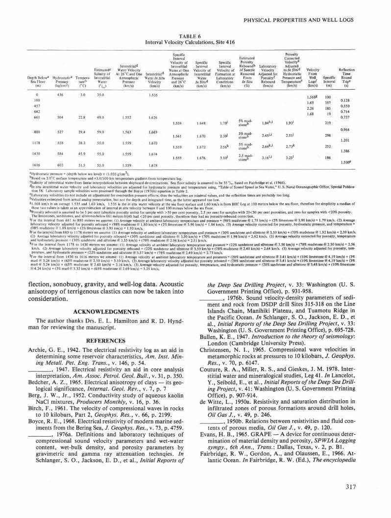
locity versus wet-bulk density (Figure 12) of the loggingdata and laboratory data were made. The velocity andwet-bulk-density values were selected at 10-meter inter-vals on the Schlumberger logs from 113 to 273 metersbelow the sea floor. In order to accurately study theporosity-rebound differences, we should recalculate thein situ velocities to 26°C and 1 atm pressure. However,for the logging data at Site 415, these corrections wouldbe less than 1 per cent of the velocity values, so we haveomitted this correction. The scatter diagram containslaboratory values at ambient temperatures (about 26 °C)and 1 atm pressure, and well-log data at in situ condi-tions. The basic contrasts of well-log velocity/densityversus laboratory velocity/density data will be relatedprimarily to porosity rebound and, perhaps, slightly torigidity of the grain-to-grain overburden pressure. How-ever, these rigidity-overburden effects should be smallfor high-porosity sediments (Hamilton, 1965).
In Figure 12 the laboratory cores appear to show sta-tistically lower densities of about 0.1 g/cm3 (equivalentto about 5 porosity units) than the in situ logs, as pre-dicted by Hamilton's (1959, 1964, 1965, 1976) consoli-
313
R. E. BOYCE
DD
V
o
Sand
Sandstone
Siltstone
Mudstone
0
ΔΔ
o
Claystone
Marl
Marlstone
Calcareous ooze
O
0
o
Chalk
Limestone
Chert and porcelanite
lmpedanc4(g.10b)/(crr/s)j
Figure 11. Laboratory-determined vertical velocity ver-sus acoustic impedance, from Sites 415 and 416.
dation rebound curves. Hamilton's (1976) data show arebound of about 2 to 5 per cent in porosity to be ex-pected from uncemented (30-60% porosity) sedimentsas the overburden pressure is released for samples from113 to 273 meters beneath the sea floor. Future testingat other sites is needed to ensure that the same litholo-gies are being studied and that the velocity logs are notactually biased on the low side. The sonic log has a shal-low depth of investigation and it could be measuring ve-locities of drill-disturbed formation or drilling muds.
IN SITU VELOCITY
Corrections to Laboratory Velocities
As discussed by Hamilton (1965), in order to calcu-late in situ from laboratory velocities we must correctfor: (1) rigidity created by grain-to-grain overburdenpressure, (2) hydrostatic pressure and temperature, and(3) porosity rebound as the overburden pressure is re-leased.
The first of these corrections will be insignificant forhigh-pososity sediment (Hamilton, 1965). However, after
the sediment consolidates some amount, perhaps up to30 per cent porosity, an overburden pressure-rigiditycorrection becomes important, whose quantity howeveris unknown. Therefore, Leg 50 data will not be cor-rected for rigidity created by overburden pressure; thus,in situ velocities corrected from laboratory data will betoo small.
The in situ temperature and hydrostatic-pressure cor-rection can be done most effectively using the Boyce(1976b) equation, listed in Table 2. For simplicity, wewill assume a calcite-and-seawater system. At labora-tory conditions, the limestone matrix has a Voigt-Reussaverage velocity of 6.45 km/s (2.72 g/cm3 density)(Christensen, 1965) and 35 per mill seawater has a veloc-ity of 1.53 km/s (1.025 g/cm3 density) ("Table of SoundSpeed In Seawater," U. S. Naval Oceanographic Of-fice, Special Publication 58; Press, 1966).
A porosity rebound of 5 per cent (5 porosity units)will be assumed for porosities greater than 30 per cent.Naturally, the porosity rebound will decrease from 5 percent at about 300 meters below the sea floor to zero atthe sea floor (Hamilton, 1976). However, the velocity/porosity relationship of sediments with high porositiesand low velocities is not unique or precise, and a largechange in porosity will have only a relatively smallchange in velocity. Therefore, the error of the 5 per centporosity will have a relatively small effect on the veloc-ity. Between 20 and 30 per cent porosity, a 2.5 per centporosity (absolute porosity units) rebound will be as-sumed, and between 0 and 20 per cent porosity, a zeroporosity rebound will be assumed.
Porosity corrections to sound velocity may be esti-mated using scatter diagrams of vertical velocity versusporosity. The measured velocity/porosity plotted pointis migrated to the in situ porosity value (and porosity-corrected velocity), in a direction approximately parallelto lines representing the velocity/porosity relationshipsof the Wood (1941) equation and the Wyllie at al. (1956)equation.
In situ calculated velocities for Leg 50 will haveundergone (1) the above porosity correction, followedby (2) the hydrostatic-pressure and temperature correc-tions.
Interval-Velocity Calculations
At Sites 415 and 416 interval velocities are estimated.They are only rough estimates, because of the hetero-geneity of lithology and the thin, alternating sequences.For each characteristic stratigraphic interval it was nec-essary to estimate percentages of a given lithology andthe average velocities for the interval. The latter werecorrected to the in situ condition, which includes correc-tions for porosity rebound, salinity of interstitial water,hydrostatic pressure, and temperatures. These correc-tions are minimal, as no adjustment is made for the ef-fect of overburden pressure on grain-to-grain rigidity. Atemperature gradient of +3.0°C per 100 meters belowthe sea floor was assumed (based on the temperature logat Site 416), and the surface temperature was estimatedat 3.0°C (based on the temperature log at Site 416 and
314
PHYSICAL PROPERTIES AND WELL LOGS
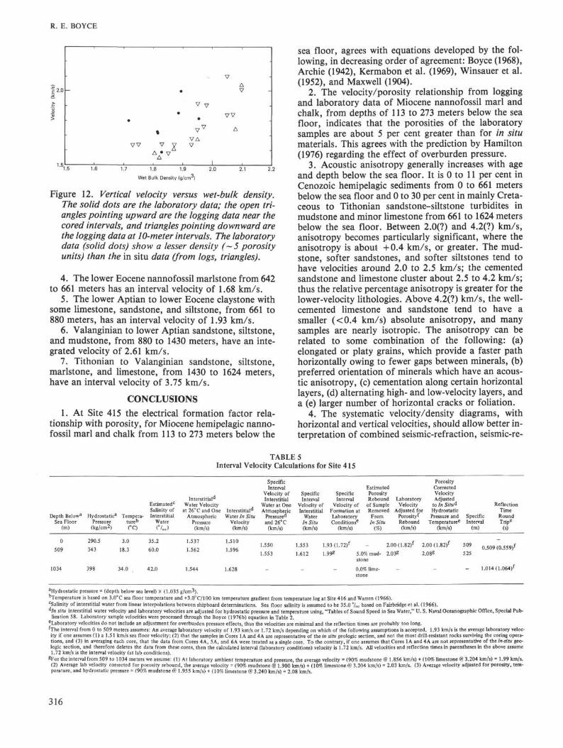
TABLE 4Electrical Resistivity, Formation Factors, and Sound-Velocity Data From the Well Logs
aTemperature of sea floor assumed to be 3.0°C based on Warren (1966), and High Resolution Temperature Log atSite 416. Water Depth = 4193 meters.
"Salinity of interstitial water from linear interpolation between shipboard determinations. Sea floor is assumed to be35%o based on Fairbridge et al. (1966).
^ h e hydrostatic pressure was calculated as = (depth below sea level) X (1.035 g/cm^).Electrical resistivity was calculated from the temperature and salinity based on Thomas et al. (1934) and the cor-rected for hydrostatic pressure by Home and Frysinger (1963) techniques.
Warren, 1966). Tables 5 and 6 give the interstitial-salin-ity assumptions, percentages of different lithologies andtheir average velocities, the correction of laboratory ve-locities to in situ values, and theoretical reflection times.
At Site 415, the calculated in situ interval velocitiesfor the Tertiary and Cretaceous sections are 2.0 km/s(or 1.82 km/s if data from Cores 1A and 4A are notconsidered characteristic of the in situ geologic section)and 2.08 km/s, respectively.
The geologic section at Site 416 is divided into sevenlayers with characteristic physical properties, based onlogging and all other available data (see site chapter, thisvolume). These layers and their estimated in situ intervalvelocities are as follows:
1. The upper Miocene, Pliocene, and Pleistocenenannofossil marls and oozes, from 0 to 100 meters, withan interval velocity of 1.57 km/s. The 100-meter bound-ary and velocity value are poorly resolved, as the sam-ples were very disturbed by the coring operation.
2. The Eocene, Oligocene, lower and middle Mio-cene sandstone, siltstone, mudstone, and minor porcel-lanite, from 100 to 457 meters. Interbedded diatom-richnannofossil marl and ooze occur in the Oligocene-Mio-cene section. This layer has an interval velocity of 1.69km/s.
3. The lower and middle Eocene mudstone, siltstone,sandstone and rare porcellanite, from 457 to 642 meters,have an interval velocity of 2.26 km/s.
315
R. E. BOYCE
2.0
1 B
-
V V
%
V
ΔΔ
•
xV
V
V
VΔV
V
V
I
V
v v
Δ
ΔV
_ J1.5 1.6 1.7 1.8 1.9 2.0 2.1 2.2
Wet Bulk Density (g/cm3)
Figure 12. Vertical velocity versus wet-bulk density.The solid dots are the laboratory data; the open tri-angles pointing upward are the logging data near thecored intervals, and triangles pointing downward arethe logging data at 10-meter intervals. The laboratorydata (solid dots) show a lesser density (~5 porosityunits) than the in situ data (from logs, triangles).
4. The lower Eocene nannofossil marlstone from 642to 661 meters has an interval velocity of 1.68 km/s.
5. The lower Aptian to lower Eocene claystone withsome limestone, sandstone, and siltstone, from 661 to880 meters, has an interval velocity of 1.93 km/s.
6. Valanginian to lower Aptian sandstone, siltstone,and mudstone, from 880 to 1430 meters, have an inte-grated velocity of 2.61 km/s.
7. Tithonian to Valanginian sandstone, siltstone,marlstone, and limestone, from 1430 to 1624 meters,have an interval velocity of 3.75 km/s.
CONCLUSIONS
1. At Site 415 the electrical formation factor rela-tionship with porosity, for Miocene hemipelagic nanno-fossil marl and chalk from 113 to 273 meters below the
sea floor, agrees with equations developed by the fol-lowing, in decreasing order of agreement: Boyce (1968),Archie (1942), Kermabon et al. (1969), Winsauer et al.(1952), and Maxwell (1904).
2. The velocity/porosity relationship from loggingand laboratory data of Miocene nannofossil marl andchalk, from depths of 113 to 273 meters below the seafloor, indicates that the porosities of the laboratorysamples are about 5 per cent greater than for in situmaterials. This agrees with the prediction by Hamilton(1976) regarding the effect of overburden pressure.
3. Acoustic anisotropy generally increases with ageand depth below the sea floor. It is 0 to 11 per cent inCenozoic hemipelagic sediments from 0 to 661 metersbelow the sea floor and 0 to 30 per cent in mainly Creta-ceous to Tithonian sandstone-siltstone turbidites inmudstone and minor limestone from 661 to 1624 metersbelow the sea floor. Between 2.0(?) and 4.2(?) km/s,anisotropy becomes particularly significant, where theanisotropy is about +0.4 km/s, or greater. The mud-stone, softer sandstones, and softer siltstones tend tohave velocities around 2.0 to 2.5 km/s; the cementedsandstone and limestone cluster about 2.5 to 4.2 km/s;thus the relative percentage anisotropy is greater for thelower-velocity lithologies. Above 4.2(?) km/s, the well-cemented limestone and sandstone tend to have asmaller (<0.4 km/s) absolute anisotropy, and manysamples are nearly isotropic. The anisotropy can berelated to some combination of the following: (a)elongated or platy grains, which provide a faster pathhorizontally owing to fewer gaps between minerals, (b)preferred orientation of minerals which have an acous-tic anisotropy, (c) cementation along certain horizontallayers, (d) alternating high- and low-velocity layers, anda (e) larger number of horizontal cracks or foliation.
4. The systematic velocity/density diagrams, withhorizontal and vertical velocities, should allow better in-terpretation of combined seismic-refraction, seismic-re-
Depth Belowa
Sea Floor(m)
0
509
1034
Hydrostatic3
Pressure(kg/cm2)
290.5
343
398
1 Tempera-ture13
CO
3.0
18.3
34.0
Estimated0
Salinity ofInterstitial
Water
C O
35.2
60.0
42.0
TABLE 5Interval Velocity Calculations for Site 415
Interstitial11
Water Velocityat 26°CandOne
AtmosphericPressure(km/s)
1.537
1.562
1.544
Interstitial0
Water In SituVelocity
(km/s)
1.510
1.596
1.628
SpecificInterval
Velocity ofInterstitial
Water at OneAtmospheric
Pressure^and 26°C
(km/s)
1.550
1.553
_
SpecificInterval
Velocity ofInterstitial
WaterIn Situ(km/s)
SpecificInterval
Velocity ofFormation atLaboratoryConditions6
(km/s)
1.553 1.93(1.72)f
1.612 1.
_
EstimatedPorosityRebound
of SampleRemoved
FromIn Situ
(%)
Laborator>Velocity
PorosityCorrectedVelocityAdjusted
to In Situd
Adjusted for HydrostaticPorosityfRebound(km/s)
2.00(1.82) f
99ß 5.0% mud- 2.03&stone
0.0% lime-stone
Pressure andTemperaturee
(km/s)
2.00(1.82)f
2.08«
_
ReflectionTime
Specific RoundInterval Tripe
(m) (s)
5 0 9 0.509 (0.559)f
525
1.014 (1.064)f
aHydrostatic pressure = (depth below sea level) X (1.035 g/cm^).bTemperature is based on 3.0°C sea floor temperature and +3.0°C/100 km temperature gradient from temperature log at Site 416 and Warren (1966).cSalinity of interstitial water from linear interpolations between shipboard determinations. Sea floor salinity is assumed to be 35.0 %° based on Fairbridge et al. (1966)."/« situ interstitial water velocity and laboratory velocities are adjusted for hydrostatic pressure and temperature using, "Tables of Sound Speed in Sea Water," U. S. Naval Oceanographic Office, Special Pub-lication 58. Laboratory sample velocities were processed through the Boyce (1976b) equation in Table 2.
laboratory velocities do not include an adjustment for overburden pressure effects, thus the velocities are minimal and the reflection times are probably too long.fThe interval from 0 to 509 meters assumes: An average laboratory velocity of 1.93 km/s or 1.72 km/s depending on which of the following assumptions is accepted. 1.93 km/s is the average laboratory veloc-ity if one assumes (1) a 1.51 km/s sea floor velocity; (2) that the samples in Cores 1A and 4A are representative of the in situ geologic section, and not the most drill-resistant rocks surviving the coring opera-tions, and (3) in averaging each core, that the data from Cores 4A, 5A, and 6A were treated as a single core. To the contrary, if one assumes that Cores 1A and 4A are not representative of the in-situ geo-logic section, and therefore deletes the data from these cores, then the calculated interval (laboratory conditions) velocity is 1.72 km/s. All velocities and reflection times in parentheses in the above assume1.72 km/s is the interval velocity (at lab conditions).
SFor the interval from 509 to 1034 meters we assume: (1) At laboratory ambient temperature and pressure, the average velocity = (90% mudstone @ 1.856 km/s) + (10% limestone @ 3.204 km/s) = 1.99 km/s.(2) Average lab velocity corrected for porosity rebound, the average velocity = (90% mudstone @ 1.900 km/s) + (10% limestone @ 3.204 km/s) 2.03 km/s. (3) Average velocity adjusted for porosity, tem-perature, and hydrostatic pressure = (90% mudstone @ 1.955 km/s) + (10% limestone @ 3.240 km/s) • 2.08 km/s.
316
PHYSICAL PROPERTIES AND WELL LOGS
TABLE 6Interval Velocity Calculations, Site 416
Depth BelowSea Floor
(m)
HydrostaticPressure(kg/cm 2)
Salinity ofTempera- Interstitial
tureb
COWater
Interstitiald
Water VelocityAt26°CandOne lnterstitiald
Atmospheric Water In SituPressure Velocity(km/s) (km/s)
SpecificInterval
Velocity ofInterstitial
Water at OneAtmospheric
Pressureand 26°C
(km/s)
SpecificInterval
Velocity ofInterstitial
WaterIn Situd
(km/s)
SpecificInterval
Velocity ofFormation atLaboratoryConditions
(km/s)
PorosityEstimatedPorosity
Rebound"of SampleRemoved
FromIn Situ
(%)
LaboratoryVelocity
Adjusted forPorosityfRebound(km/s)
CorrectedVelocitye
Adjustedto In Sitùá
HydrostaticPressure and
Temperaturee
(km/s)
VelocityFromWellLogsf
(km/s)
ReflectionTime
Specific RoundInterval Tripe
(m) (s)
0
100
457
642
661
880
1178
1430
1616
3.0 35.0
22.8 49.0
1.535
527
558
584
603
29,4
38.3
45.9
51.5
59.0
55.0
55.0
55.0
1.552
1.563
1.559
1.559
1.559
1.5688
1.69
2.26
1.68
100
357
185
19
0.128
0.550
0.714
0.737
1,669
1.670
1.674
1.678
1.561
1.559
1.559
1.670
1.672
1.676
2.39J
2.56k
3.101
5% mudstone"
5% mud-stone"
stone"
2.5 mud-stone11
1.84"-'
2.45J j
2.64k•>
1.931
2.51J
2 . 7 3 k
3.25
aHydrostatic pressure = (depth below sea level) × (1.035 g/cm3).bBased on 3.0°C surface temperature and +3.0/100 km temperature gradient from temperature log.cSalinity of interstitial water from linear interpolations between shipboard determinations. Sea floor salinity is assumed to be 35 7°o based on Fairbridge et al. (1966).d/rt situ interstitial water velocity and laboratory velocities are adjusted for hydrostatic pressure and temperature using, "Table of Sound Speed in Sea Water," U. S. Naval Oceanographic Office, Special Publica-
tion 58. Laboratory sample velocities were processed through the Boyce (1976b) equation in Table 2.laboratory velocities do not include an adjustment for overburden pressure effects; thus the velocities are minimal values, and the reflection times are probably too long.'Velocities estimated from actual analog presentation, but not the depth and integrated time, as the latter appeared too low.§1.568 km/s is an average 1.5.35 and 1.60 km/s. 1.535 is the in situ water velocity at the sea floor surface and 1.60 km/s is from BHC Log at 100 meters below the sea floor, therefore for simplicity a median ofthese two values is taken as an approximation of interval in situ velocity between 0 and 100 meters below the sea floor.
"Porosity rebound is assumed to be 5 per cent (absolute porosity units) for sample with >30 per cent porosity, 2.5 per cent for samples with 20<30 per cent porosities, and zero for samples with <20% porosity.The limestones, sandstones, and siltstones below 661 meters depth had <20 per cent porosity, therefore they had no porosity-rebound correction.
'For the interval from 661 to 880 meters we assume: (1) Average velocity at ambient laboratory temperature and pressure = (98% mudstone @ 1.75 km/s) + (2% limestone @ 3.90 km/s) = 1.79 km/s. (2) Averagelaboratory velocity adjusted for porosity rebound = (98% mudstone @ 1.80 km/s) + (2% limestone @ 3.90 km/s) = 1.84 km/s. (3) Average velocity corrected for porosity, hydrostatic pressure, and temperature =(98% mudstone @ 1.89 km/s) + (2% limestone @ 3.95 km/s) = 1.93 km/s.
JFor the interval from 880 to 1178 meters we assume: (1) Average velocity at ambient laboratory temperature and pressure = (30% sandstone and siltstone @ 3.50 km/s) + (70% mudstone @ 1.92 km/s) = 2.39 km/s.(2) Average laboratory velocity adjusted for porosity rebound = (30% sandstone and siltstone @ 3.50 km/s) + (70% mudstone @ 1.98 km/s) = 2.42 km/s. (3) Average velocity corrected for porosity, temperatureand hydrostatic pressure = (30% sandstone and siltstone @ 3.55 km/s) + (70% mudstone @ 2.06 km/s) = 2.51 km/s.
kFor the interval from 1178 to 1430 meters we assume: (1) Average velocity at ambient laboratory temperature and pressure = (22% sandstone and siltstone @ 3.50 km/s) + (78% mudstone @ 2.30 km/s) = 2.56km/s. (2) Average laboratory velocity adjusted for porosity rebound = (22% sandstone and siltstone @ 3.50 km/s) + (78% mudstone @ 2.40 km/s) = 2.64 km/s. (3) Average velocity adjusted for porosity, tem-perature, and hydrostatic pressure = (22% sandstone and siltstone @ 3.57 km/s) + (78% mudstone @ 2.49 km/s) = 2.73 km/s.
'For the interval from 1430 to 1616 meters we assume: (1) Average velocity at ambient laboratory temperature and pressures = (28% sandstone and siltstone @ 3.41 km/s) + (10% limestone @ 4.19 km/s) + (3%marl @ 3.24 km/s) + (65% mudstone @ 2.50 km/s) = 3.10 km/s. (2) Average laboratory velocity adjusted for porosity rebound = (28% sandstone and siltstone @ 3.41 km/s) + (10% limestone @ 4.19 km/s) + (3%marl @ 3.24 km/s) + (65% mudstone @ 2.60 km/s) = 3.16 km/s. (3) Average velocity adjusted for porosity, temperature, and hydrostatic pressure = (28% sandstone and siltstone @ 3.48 km/s) + (10% limestone@ 4.24 km/s) + (3% marl @ 3.32 km/s) + (65% mudstone @ 2.69 km/s) = 3.25 km/s.
flection, Sonobuoy, gravity, and well-log data. Acousticanisotropy of terrigenous elastics can now be taken intoconsideration.
ACKNOWLEDGMENTS
The author thanks Drs. E. L. Hamilton and R. D. Hynd-man for reviewing the manuscript.
REFERENCESArchie, G. E., 1942. The electrical resistivity log as an aid in
determining some reservoir characteristics, Am. Inst. Min-ing Metall. Pet. Eng. Trans., v. 146, p. 54.
, 1947. Electrical resistivity an aid in core analysisinterpretation, Am. Assoc. Petrol. Geol. Bull., v. 31, p. 350.
Bedcher, A. Z., 1965. Electrical anisotropy of clays — its geo-logical significance, Internat. Geol. Rev., v. 7, p. 7
Berg, J. W., Jr., 1952. Conductivity study of aqueous kaolinNaCl mixtures, Producers Monthly, v. 16, p. 36.
Birch, F., 1961. The velocity of compressional waves in rocksto 10 kilobars, Part 2, Geophys. Res., v. 66, p. 2199.
Boyce, R. E., 1968. Electrical resistivity of modern marine sed-iments from the Bering Sea, /. Geophys. Res., v. 73, p. 4759.
, 1976a. Definitions and laboratory techniques ofcompressional sound velocity parameters and wet-watercontent, wet-bulk density, and porosity parameters bygravimetric and gamma ray attenuation technqies. InSchlanger, S. O., Jackson, E. D., et al., Initial Reports of
the Deep Sea Drilling Project, v. 33: Washington (U. S.Government Printing Office), p. 931-958.
., 1976b. Sound velocity-density parameters of sedi-ment and rock from DSDP drill Sites 315-318 on the LineIslands Chain, Manihiki Plateau, and Tuamotu Ridge inthe Pacific Ocean. In Schlanger, S. O., Jackson, E. D., etal., Initial Reports of the Deep Sea Drilling Project, v. 33:Washington (U. S. Government Printing Office), p. 695-728.
Bullen, K. E., 1947. Introduction to the theory of seismology.London (Cambridge University Press).
Christensen, N. I., 1965. Compressional wave velocities inmetamorphic rocks at pressures to 10 kilobars, J. Geophys.Res., v. 70, p. 6147.
Couture, R. A., Miller, R. S., and Gieskes, J. M. 1978. Inter-stitial water and mineralogical studies, Leg 41. In Lancelot,Y., Seibold, E., et al., Initial Reports of the Deep Sea Drill-ing Project, v. 41: Washington (U. S. Government PrintingOffice), p. 907-914.
de Witte, L., 1950a. Resistivity and saturation distribution ininfiltrated zones of porous formations around drill holes,Oil Gas J., v. 49, p. 246.
, 1950b. Relations between resistivities and fluid con-tents of porous media, Oil Gas J., v. 49, p. 120.
Evans, H. B., 1965. GRAPE — A device for continuous deter-mination of material density and porosity, SPWIA Loggingsympy., 6th Ann., Trans.: Dallas, Texas, v. 2, p. Bl.
Fairbridge, R. W., Gordon, A., and Olaussen, E., 1966. At-lantic Ocean. In Fairbridge, R. W. (Ed.), The encyclopedia
317
R. E. BOYCE
of oceanography: New York (Reinhold Publishing Corp.),v. 1, p. 56.
Greene, E. S., 1962. Principles of physics: Englewood Cliffs,N. J. (Prentics Hall Inc.).
Hamilton, E. L., 1959. Thickness and consolidation of deepsea sediments, Geol. Soc. Am. Bull., v. 70, p. 1399.
, 1964. Consolidation characteristics and relatedproperties of sediments from experiental Mohole (Guada-lupe site), /. Geophys. Res., v. 69, p. 4257.
1965. Sound speed and related physical propertiesof sediments from experimental Mohole (Guadalupe site),Geophysics, v. 30, p. 257.
, 1970. Reflection coefficients and bottom losses atnormal incidence computed from Pacific sediment proper-ties, Geophysics, v. 35, p. 995.
, 1971. Prediction of in situ acoustic and elastic prop-erties of marine sediments, /. Geophys., v. 36, p. 266.
_, 1976. Variations of density and porosity with depthin deep-sea sediments, J. Sediment. Petrol., v. 46, p. 280.
Home, R. A., 1965. The physical chemistry and structure ofsea water, Water Resources Res., Second quarter, v. 1,p. 263.
Home, R. A. and Courant, R. A., 1964. Application ofWalden's rule to the electrical conduction of sea water, /.Geophys. Res., v. 69, p. 1971
Home, R. A. and Frysinger, G. R., 1963. The effect of pres-sure on the electrical conductivity of sea water, /. Geophys.Res., v. 68, p. 1967.
Howell, B. F., Jr., 1953. Electrical conduction in fluid satu-rated rocks, Part I, World Oil, v. 136, p. 113.
Keller, G. V., 1951. The role of clays in the electrical conductiv-ity of the Bradford Sand, Producers Monthly, v. 15, p. 23.
, 1966. Electrical Properties of Rock and Minerals. InClark, S. P. (Ed.), Handbook of physical constants: NewYork (Geol. Soc. Amer., Mem. 97), p. 553.
Keller, G. V. and Frischknecht, F. C , 1966. Electrical meth-ods in geophysical prospecting: New York (PergamonPress).
Kermabon, A., Gehin, C , and Blavier, P., 1969. A deep-seaelectrical resistivity probe for measuring porosity and densi-ty of unconsolidated sediments, Geophysics, v. 34, p. 554.
Laughton, A. S., 1957. Sound propagation in compactedocean sediments, Geophysics, v. 22, p. 233.
Maxwell, J. C , 1904. Electricity and magnetism: Oxford(Clarendon Press), v. 1, 3rd ed.
Nafe, J. E. and Drake, C. L., 1957. Variation with depth inshallow and deep water marine sediments of porosity den-sity and the velocities of compressional and shear waves,Geophysics, v. 22, p. 523.
, 1963. Physical properties of marine sediments. InHill, M. N. (Ed.), The sea: New York (Interscience), v. 3,p. 749.
Patnode, H. W. and Wyllie, M. R. J., 1950. The presence ofconductive solids in reservoir rocks as a factor in electric loginterpretation, /. Petrol. Tech., v. 2, p. 42.
Press, F., 1966. Seismic Velocities. In Clarks, S. P. (Ed.),Handbook of physical constants: New York (Geol. Soc.Am. Memoir 97), p. 195.
Schlumberger Ltd., 1972. Log interpretation charts: New York(Schlumberger Ltd.).
Scholl, D. W., 1963. Techniques for removing interstitialwater from coarse grained sediments for chemical analyses,Sedimentology, v. 2, p. 156.
Siever, R., Garrels, R. M., Kanwisher, J., and Berner, R. A.,1961. Interstitial waters of Recent marine muds off CapeBode, Science, v. 134, p. 1071.
Siever, R., Kevin, C. B., and Berner, R. A., 1965. Composi-tion of interstitial waters of modern sediments, /. Geol.,v. 73, p. 39.
Thomas, B. D., Thompson, T. G., and Utterback, C. L.,1934. The electrical conductivity of sea water, Conseil, In-ternat. Explor. Mer., v. 9, p. 28.
Warren, B., 1966. Oceanography, physical In Fairbridge, R.W. (Ed.), The encyclopedia of oceanography: New York(Reinhold Publishing Corp.), v. 1, p. 56.
Winsauer, W. O. and McCardell, W. M., 1953. Ionic double-layer conductivity in reservoir rock, Am. Inst. MiningMe tall. Petrol. Eng. Trans., v. 198, p. 129.
Winsauer, W. O., Shearin, H. M., Jr., Masson, P. H., andWilliams, M., 1952. Resistivity of brine-saturated sands inrelations to pore geometry, Am. Assoc. Petrol. Geol. Bull.,v. 36, p. 253.
Wood, A. B., 1941. A Textbook of sound: New York (Mac-Millan).
Wyllie, M. R. J., 1955. Role of clay in well-long interpretationon clays and clay technology, July, 1952, Cal. Div. MinesBull., v. 169, p. 282.
Wyllie, M. R. J. and Gregory, A. R., 1953. Formation factorsof unconsolidated porous media: influence of particleshape and effect of cementation, /. Petrol. Tech., v. 198,p. 103.
Wyllie, M. R. J. and Southwick, P. F., 1954. An experimentalinvestigation of the S. P. and resistivity phenomena in dirtysands, J. Petrol. Tech., v. 6, p. 44.
Wyllie, M. R. J., Gregory, H. R., and Gardner, L. W., 1956.Elastic waves in heterogeneous and porous media, Geo-physics, v. 21, p. 41.