SoundPLAN noise Update News 7 - Whidbey Telecom · Update News 7.4 March 2015 4 Overview of the...

SoundPLAN noise

Update News 7.4

SoundPLAN GmbH

March 2015

Update News 7.4

March 2015

Contents i

Contents

New developments in SP 7.4 - noise 3

Highlights 3

Overview of the Changes 4

Details of innovations and changes 19 Directivity library 19 Properties Industrial building 22 Import photo points with GPS data 25

Wind Turbine 25 Variables in formulas for Spreadsheet and file operations 26 Calculate Sound Power from Measured Data 27 Define emissions via formulas 29

Output of geo-referenced bitmaps 34 Rotated bitmaps 35 Drawing Grid Maps- and Meshed Maps in geometry bitmap 35

Implemented calculation standards 36

Update News 7.4

March 2015

Highlights 3

New developments in SP 7.4 - noise

Highlights 2D- and 3D-directivity are completely re-designed

Buildings and industrial buildings can now float and allow noise to pass underneath

The industrial building was re-designed

Highlights in various modules:

Roads and railway: Emission calculation now integrated into the property dialog screen

Import of picture locations with GPS information

Calculate the sound power level from measurement points

The version 7.4 also has many changes for the air pollution modeling that are described in their own separate update text.

Update News 7.4

March 2015

4 Overview of the Changes

Overview of the Changes General

o Revised hardware recommendations: As the pre-calculation in the calculation core (calculation of emissions, searching DGM triangles, preparing buildings …) are not (yet) designed to make use of multiple core processors, processors with a very high operating frequency (or with turbo boost) will yield the highest throughput of the entire system. For this reason the clock speed at the moment is for SoundPLAN more important than the number of cores in a processor.

o The „decisive floor“ entry in the object settings for buildings is obsolete and was purged in Geo-database, Result tables, Spreadsheet and the Graphics. In den Result Tables you can filter instead for the „HIGHEST LIMIT EXCEEDANCE PER FACADE“.

o With Distribute Updates you can now also distribute Libraries, System Libraries, System Files and the Manuals/Help Files. Click on the list to activate what you want to distribute. Distribute Updates will remember for each SoundPLAN version the path that is used to save these files. In a logbook warnings and errors of the installation of the update will be displayed with red color (for example if a computer was running while attempting to distribute the update.

Geo-Database

o Re-design of the Industrial Building. The Overview:

- The diffusion parameter Cd can now be entered flexibly for single broadband entries (ISO 12354).

- The source geometry can attain multiple different configurations, typical example „Door Open“ - „Door Closed“.

- Embedded point and line sources can be directly assigned to the source derived from the facade if the exact geometrical form (location) is not known or not relevant. For this it is now possible to enter a point or line source and assign it to the area. This additional source is used to calculate the total emission from the area source (for levels defined as per square meter or for calculations Hallin/Hallout).

- Industrial buildings now can have the marker to be “floating”, i.e. detached from the ground where noise can pass underneath unimpeded. In one of the next small updates it is planned to also make the industrial building radiate noise through the bottom if the marker “floating” has been set. With this feature it will be possible to model boxes with compressors in an industrial rack where all sides, including the bottom radiate noise.

- The Lmax can now also be processed for sources embedded in the facade of an industrial building.

For a detailed description see page 22.

o New object type and calculation method „Wind energy turbines “, see page 25.

o The Emission dialog for roads and railway sources have moved into a separate tab in the main attribute definitions instead of a button that opens a separate window. The main advantage is that you now can click through the different emission definitions with traffic volume, speeds and surface dependent additions.

Update News 7.4

March 2015


As soon as the box EMISSION CALCULATED is checked in the tab Emission / Station, the emission calculation is presented as a tab of its own (Exception: Road standards based on the „old“ emission calculation (for example RLS-90*** in old projects). For these the emission calculation is presented as a separate dialog.

o In the selection of road cross-sections the new standard road cross-sections for Germany (RAL 2012, RAA 2008) are incorporated.

o The separate definition of the lane width for the left and right is now possible even for roads with a single emission band.

Enter the lane width left and right of the master alignment string. For old projects, half the total lane width is assigned to the left and to the right lane.

o Modeling of bridges has changed:

In case you have to model bridges for multiple single lane roads or multiple railways, SP 7.4 expects the bridge definition for each lane or track. The individual bridges should overlap if it is one bridge in the model.

With this change the program avoids problems that occur when roads cross each other and the terrain is „confused“ what road is representing the terrain and what is detached and thus on the bridge.

o The parameters to incorporate the railway axis into the DGM are now available in the railway attribute entry.

By default the terrain is assumed to be 60 cm below the rail head; elevation points along the track (by default 1.8 meters left and 1.8 meters right of the track alignment) are not used in the calculation of the DGM triangulation.

o The procedures entering groups for industrial sources and parking lots is now more transparent:

o For industrial sources with an assigned directivity, the definition of the directivity is now more understandable. Especially for the 3D directivity it is much easier. The main radiation direction can be adjusted with a mouse click (Ctrl+left mouse button).

o Industrial sources can be absolute or relative in their Z component of the coordinate. Which one of the definitions a particular source is set to, is now visible

Update News 7.4

March 2015


in the top frame of the sources attribute definition. You will see either (ABSOLUTE

HEIGHT) or (RELATIVE HEIGHT).

In addition to the passive presentation you will also find the control for TERRAIN

REFERENCE in the first tab of the so the source definition.

o Floating buildings and industrial buildings: With the click box BUILDING FLOATS ABOVE

GROUND (NOISE CAN PASS UNDERNEATH) the base of the building is not connected to the ground.

For the calculation only the screening is regarded not the reflections between the ground and the bottom of the buildings! If you want to regard the reflections between the ground and the bottom of the buildings correctly, you need to simulate the interaction with an Indoor Noise Calculation and manually generate an area source at the bottom of the building and assign it the sound power that is equal to the reflected noise components between the ground and bottom of the building. Please also observe that any floating structure will significantly increase the calculation time. For that reason floating objects should be used sparingly for detail calculations.

With this switch several new modeling options become possible:

- Buildings where higher floors are bigger than the ground floor

- Modelling of passageways under buildings and entries to courtyards

- Buildings that have different usages, floor heights and reflection losses

- Industrial buildings with multiple floors (parking garages)

- Aggregates in (compressors, engines…) in containers on industrial racks (the noise radiation of the bottom of the box will be available shortly)

In order to allow receivers in stacked buildings to be labeled continuously, the label for the lowest floor was amended.

Update News 7.4

March 2015


o Improvements in the Attribute Explorer:

- Right mouse button on the header: REMOVE COLUMN PERMANENTLY.

- All selectable properties are available as selection lists (for example the text alignment.

- Texts from selection lists can be used in formulas.

- Color, font, text style and alignment of Geotexts are easily selectable.

- New statistics function "Count" which sums up the number of different properties in a column.

- Number of selected rows in the status bar.

- The column type (text, float …) is shown as hint when you move the cursor over the column header.

- Search + Replace (F4) in text columns.

o Calculating receivers in the Geo-Database: The first call to this facility will open the calculation settings so that you can check them.

When you calculate receivers from the Geo-Database next time, the parameters from the last run will be used, check or modify them by clicking

on the wheel symbol.

The logbook for the calculation is opened with a button, when hints, warnings and errors were found in the calculation. They are highlighted in cursive fonts, blue for hints, red-normal for warnings and red-bold for errors.

o Preflight and logbook are redesigned. Open the geometry check with TOOLS ->

PREFLIGHT. The logbook will open automatically.

The logbook is no longer on top of the Geo-Database canvas and can now be moved at will, even to a secondary screen. When clicking on a warning or an error message, the coordinate(s) where the warning/error was detected will be marked with circles. By double clicking the object zooms to its max size for a complete display.

With a right mouse click you can select what Preflight shall note in the logbook. Errors always will be shown, hints and warnings are optional.

o Generating new own graphics object types was simplified. Click on the symbol EDIT

OBJECT TYPES in the dialog EDIT -> GRAPHICS OBJECT TYPE.

Update News 7.4

March 2015


o GEO-TOOLS -> MORE BUILDING TOOLS -> SELECT BUILDINGS BY SPREADSHEET. With this Geo-Tool you can use a Boolean column from the spreadsheet to assign buildings and receivers a criterion to mark/unmark the object (if the Boolean value is true, the object is marked). Buildings marked this way can for example be moved to a different Geofile or can be assigned a different graphics object type.

o GEOTOOLS -> MORE BUILDING TOOLS -> TRANSFER AREA USAGE TO BUILDINGS. With this Geo-Tool the zoning definition from objects of the object type "usage areas" is transferred to the appropriate attribute of the marked building objects.

Mark the area usages and all buildings that you want to define the area usage attribute. If no buildings are marked, all buildings contained in a usage area will have the attribute set.

o GEOTOOLS -> MORE GEOMETRY TOOLS ->UNITE AREAS. Generates a hull around all marked areas (regardless of the object type) to generate a bigger area containing all marked sub areas. This can be used for example to use areas of city boroughs to generate a calculation area. Holes (areas not part of a marked area but totally encapsulated) and overlapping areas are ignored. The resulting area is of the type of general area and can then be converted into any other type.

o The algorithm of the Geo-Tool CONNECT OBJECTS was re-worked and improved. The name of the object is deleted if multiple objects are concatenated with the function.

o SPLIT OBJECTS. For road and railway objects the mile post is transferred if the first road/railway had the value for the mile post set.

o GEOTOOLS -> EVALUATE OBJECT HEIGHT FROM TOP EDGE now can be applied for industrial buildings, too. For buildings and industrial buildings choose the appropriate reference to the ground:

o TOOLS -> CREATE GEOTEXTS FROM ATTRIBUTES. With this tool you can generate texts from any object. Mark the objects for which you wish to generate descriptive texts from the attributes.

If needed, select a different object type and the attribute. Under options choose the TEXT HEIGHT in [m] (world coordinates). For area type objects all other options are grayed out, the reference point for the text is always the center of the area. For line type objects choose the VERTICAL ALLIGNMENT of the geo texts along the line, depending on the data entry direction. Another option is to have a vertical displacement (MOVE VERTICAL). For point type objects the texts by default will be placed to the right of the object, the vertical alignment is centered. For point objects the placement can be set with VERTICAL ALIGNMENT, or with MOVE HORIZONTAL /

VERTICAL.

Update News 7.4

March 2015


The newly generated geometry texts „know" the object and the attribute they were generated from. If you generate a new geometry text for the same object and attribute, the previous text is deleted.

o Rotating objects was improved. Mark the objects you want to rotate and activate VIEW -> SHOW DIALOG "EDIT SELECTED OBJECTS" (Shift+Ctrl+R).

You can either enter the rotation angle in DEGREES [°] via the keyboard or use the arrows next to the entry field to get to the desired angle. The field INC sets the increment for the angle field. Enter 0° to reset the rotation. You can leave the window open parallel to the normal data entry window. (The rotation with Ctrl + left mouse button on the group center marker is also still an option for the rotation.)

o Data imported to the project with „Import -> SoundPLAN“ are selected so that they can be recognized and more directly processed.

Imported data are placed centered in the active view. This way you can import a discount store and place it centered into the piece of property so that additional correction of the location is minimal.

o When importing road and railway Geo-files and no road or railway data is present in the project, the road/railway library will be imported. If roads and railway lines are already present, the existing libraries will not be overwritten. A message will inform you that it is possible to have discrepancy between the road/railway type definitions. Please check your emission calculation in this case.

o For the DXF-Export you now can choose if you want to export the data into a separate layer per geo-file or per object type.

o Shape import for 3D-buildings as triangles was modified so that the 3D-buildings can be imported more quickly. It is no longer a requirement to have level ground under the building. SoundPLAN now uses all triangles projected to the terrain surface to generate a continuous hull. For this reason now even balconies are part of the buildings floor plan.

If not further detailed settings are made, the lowest z-coordinate of the building will be used defining the elevation of the lowest floor slab. Often there is an extra column in the dbf-file defining the floor elevation. A more accurate model can be made when you assign the field h1 to this value (before doing this, check the data in the dbf file).

o Import of Photos with GPS data, see page 25.

Calculation Core

o When a calculation is finished, the Calculation Core no longer moves to the foreground of the desktop, instead you will see a status message with the relevant information.

o For the settings of the tolerance in the calculation settings, 0.1 is now the smallest value. The settings for the group level became obsolete. When you activate the

Update News 7.4

March 2015


generation of detail result tables, the tolerance is automatically set to „tolerance for every source contribution" to avoid situations where the level of a contribution changes when a source is amended or taken out.

o Up to and including version 7.3 for most of the standards calculations were performed on rounded third octave band frequencies. Due to the extension to low frequencies and a harmonization SoundPLAN version 7.4 switches to frequencies calculated by band numbers.

Hereby applies for the frequency f [Hz] = 10 ^ (0.1*b), with band number b.

b 13 14 15 16 17 18 19 20 21 22 23 24 25 26

Nominalfrequenz 20 25 31 40 50 63 80 100 125 160 200 250 315 400

10^(0.1*b) 19.95 25.12 31.62 39.81 50.12 63.10 79.43 100.00 125.89 158.49 199.53 251.19 316.23 398.11

b 27 28 29 30 31 32 33 34 35 36 37 38 39 40

Nominalfrequenz 500 630 800 1000 1250 1600 2000 2500 3150 4000 5000 6300 8000 10000

10^(0.1*b) 501.19 630.96 794.33 1000.00 1258.93 1584.89 1995.26 2511.89 3162.28 3981.07 5011.87 6309.57 7943.28 10000.00

This has effects especially on air absorption and on weighting filters dB(A)..dB(D) and may lead to slight deviations in the results compared to previous versions of SoundPLAN. The weighting filters have been calculated from complex transfer functions and tabularized with three decimals.

o If the presentation of the Facade Noise Map does not present the facades or does not fill the building, often this is due to the fact that buildings have been copied and thus the building ID from the Façade Noise Map no longer matches the building ID of the geometry from the situation or Geofile. To rectify this problem, open the calculation core, right click on the calculation run in question and select the action RESET BUILDING ID from the menu. After the confirmation, all building IDs in the Facade Noise Map will be reset to the value found in the building geometry.

o Extract DGM via an area: When a DGM for the entire project is already present and you want to restrict the DGM to cover only a portion of the entire DGM, you can clip the DGM. In the Geo-Database define an area (calculation area or general area) and save it in a Geo-file of its own.

In the Calculation Core select the calculation type CLIP DGM from the category GEOMETRY.

Enter the Geofile with the area functioning as the clipping template and the existing DGM and in the bottom of the definition box the number for the part DGM to be created. Additionally you can enter the size of a buffer around the selected clip area so that the elevation supply for the part area is assured.

o Now it is possible to calculate the Lmax for vertical area sources.

o The Schall 03-2012 was implemented and is now available if you select the standard Schall 03-2012.

For the emission calculation there are 2 libraries to your disposal:

Schall03-2012: Vehicle categories

Schall03-2012: Train setup

In the system-train setup you find various standard passenger trains that are compiled from the vehicle categories defined by the German Rail environmental center (BUZ=Bahnumweltzentrum).

Update News 7.4

March 2015


In praxis (for Germany) the trains will be available in the form of train schedule data sheets from BUZ. These settings are subject to change when the time table changes between summer schedule and winter schedule.

In accordance to the standard the calculation must include the third order reflections; the train bonus no longer applies.

Distributed Computing

Via a timer you can activate PCs for certain time periods (PCs that for example at night would be idling).

Library

o The frequency range in the Emission library has been amended to cover lower frequencies, the range is now (1Hz-20kHz).

The wave length is the only parameter for the screening, it can be calculated for any frequency. The air absorption in accordance to the ISO 9613 / 1 also can be calculated for any frequency.

Ground effect: For standards such as the Nord2000, the ground effect is calculated explicitly as a function of the frequency, therefore the ground effect is valid for any frequency. For standards based on the ISO 9613 or CONCAWE where the ground effect is only defined for certain octave middle frequencies, the value of the lowest defined freqency is used, because the ground effect changes only insignificantly below this lowest octave band.

o The CLF Import (Common Loudspeaker Format) is now incorporated into the emissions library. The frequencies of the loudspeaker are imported and a directivity element (with the same name) is generated for the directivity library.

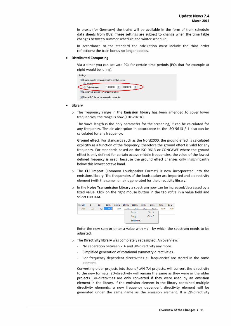
o In the Noise Transmission Library a spectrum now can be increased/decreased by a fixed value. Click on the right mouse button in the tab value in a value field and select EDIT SUM.

Enter the new sum or enter a value with + / - by which the spectrum needs to be adjusted.

o The Directivity library was completely redesigned. An overview:

- No separation between 2D- and 3D-directivity any more.

- Simplified generation of rotational symmetry directivities.

- For frequency dependent directivities all frequencies are stored in the same element.

Converting older projects into SoundPLAN 7.4 projects, will convert the directivity to the new formats. 2D-directivity will remain the same as they were in the older projects. 3D-diretivities are only converted if they were used by an emission element in the library. If the emission element in the library contained multiple directivity elements, a new frequency dependent directivity element will be generated under the same name as the emission element. If a 2D-directivity

Update News 7.4

March 2015


element was assigned to an emission element as a vertical directivity a new 3D-rotation symmetry directivity element will be generated. Detailed description on page 19ff.

o New library for Li(Calc) day history frequencies

When there are multiple sources present in an industrial building, each with a spectrum and a day history, each receiver in the factory hall has a frequency spectrum of its own that can vary by the hour. For Grid Noise Maps this is not relevant but it is for receivers close to the halls walls that are used to drive the Hallin/Hallout calculation. For the calculation of the indoors noise levels for the sake of calculating transmission through the wall and calculating the propagation into the environment, these data are now stored in the Li(Calc) day histogram spectra library. This lib contains the day history frequencies as a calculation result of an indoor simulation.

Up until now the results were hosted in the normal emission library, which sometimes clattered the library. With the new day history frequency library the structure is clear and the noise levels outside are correct in their representation of the day histories of individual sources indoors.

o The Library printouts were redesigned.

o Sort according to element name or element number is now possible in all libraries by clicking on the column header.

Result Tables

o In the single receiver table you now can apply filters to show either the highest exceedance (excess noise level above the noise limit) for each façade or the highest noise level. With the right mouse button activate SELECT FILTER and select the HIGHEST

LIMIT EXCEEDANCE PER FACADE or the HIGHEST LEVEL PER FACADE.

Right mouse button -> SELECT FILTER respective SHOW ALL you toggle the view.

These filters previously were connected to the „decisive floor“. For older tables the exceedance of the noise limit is calculated automatically and the previous selection is overwritten.

o Transfer column setup, table layout, page format and headers / footers in one step from the active result to all other open results with FILE -> TRANSFER TABLE SETTINGS TO

OPEN RESULTS.

It is therefore sensible to first design all tables of one result as desired, then load further results and transfer the table settings.

Update News 7.4

March 2015


Spreadsheet

o Extended formulas with variables, see page 26

o [Noise Mapping Toolbox] It is now possible to import multiple variants of an inhabitant or area statistics into a single area table.

To interconnect multiple statistics, select the column type TABLE -> ADD COLUMN -> INTERVAL. To compare the effectiveness of different noise control measures, the difference between the intervals is not a good decision criterion by itself. In addition it is recommended to calculate the sum of the noise effected persons for each variant. Enter the formula SUMXstatisticsscolumn (no blanks permitted) in a value column.

Graphics

o For the presentation of geo-referenced bitmaps in combination with area type results you can opt to set the object type to TRANSPARENT and SCHADED for the result type and to NORMAL for the geometry bitmap. This combination was found to work best with PDF drivers that previously had problems with superimposed maps.

A description of how to print geo-referenced bitmaps you can read from page 34.

o For the presentation of the Facade Noise Map it is now possible to present the object number of the processed building as a Building reference in addition to the receiver points.

In the map object types of the Facade Noise Map activate the sub-object-type BUILDING REFERENCE POINT.

Update News 7.4

March 2015


Select if the reference point shall be positioned IN THE BUILDING or on a line PERPENDICULAR TO THE FIRST FACADE or THE BISECTING LINE BETWEEN THE FIRST AD THE LAST

FACADE. For the last 2 options define the DISTANCE between the building reference point and the building corner and additionally the LINE WIDTH. The building corner can be marked with an ARROW. The building reference point can be drawn in different ways depending on the sub object type for buildings with / without noise limit violation.

Via the delivered template "Spreadsheet with building reference.ntt" for the spreadsheet you can connect the graphical presentation to the receivers in the table.

o The Legend was re-worked: Sub objects (for example in tunnels or the central reservation), for which no extra data are available, are no longer written into the legend.

When using templates, the legend often contains elements that are not present in the sheet. You now find a button to mark all elements not included

in the sheet.

With Ctrl + left click on a legend entry the entry is marked / respective unmarked. This is useful for example if noise protection walls are present in the project but the current sheet does not have a noise protection wall in the visible area.

All marked legend entries can then be deleted commonly with the DELETE

BUTTON.

Improvements of the legend for plan object types:

Activating / deactivating the legend text in the map object types will insert/delete them in the legend immediately.

o Changes in the Object type files:

When you have two object type files open, you can use Drag&Drop or the button TAKE OVER LAYOUT to copy the layout of a selected (one or multiple)

object type to a secondary object type file. The layout is only copied if the type is already present in the secondary layout type file. If you want to copy the layout even for layout types that do not have an equivalent in the secondary layout type file, you need to hold the Shift key while dragging the layout types to the second file. In this case the new object types will be generated in the secondary layout type file.

If only a single object type file is opened, the layout of marked object types will be transferred to the object type file of the next higher hierarchy (from map to project or from project to the global settings).

Update News 7.4

March 2015


Transferring the layout of object types to other sheets in the project: Open the sheet tree (F6). Open the map object type file that you want to use as the master, click on individual object types or entire branches (using the Shift and Ctrl keys) to mark them. Now click on all sheets in the sheet tree that you want to transfer the layout to.

The layout of the object type road and all object types in the branch „Environment“ are to be transferred to the marked sheets on the left

With the button TAKE OVER IN SHEET TREE, the layout is transferred to the object types of the sheets if the object type is included in the particular sheet.

o In the map object types all objects not used or not included in the legend will be displayed gray and cursive.

With the red DELETE CROSS these obsolete object types can be deleted from the plan object types (except for sub-objects such as central reservation and

bridges).

o Receivers and point sources now have an additional option in the 3D Graphics to draw a line from the point type object to the ground. This allows a better understanding of the position in space. To activate this feature, go to the object types tab 3 D Graphics and activate LINE TO GROUND.

Update News 7.4

March 2015


o The object tpyes define inserted noise sources on an industrial building as sub-object types of the industrial building so that these sources can be displayed in different colors.

o Printing preview and printing was improved. If the borders are exceeding the printable area, the printed part will be centered on the sheet rather than cut only on the right and the bottom area. The non-printable area is hatched with red lines in the print preview.

o If a DGM in the graphic is supposed to be shown with elevation contours, you now can different legend entries for main, middle and intermediate intervals.

o With the grid and contour line export you can transform the coordinates into another coordinate and reference system.

Update News 7.4

March 2015


Tools Noise Mapping Tools

o The tile manager and the selection of individual tiles were improved. In the tile manager extra information about the results of individual tiles is visualized:

With a quick glimpse you can see if a tile was not calculated because there were no receivers in the tile or because no sources were found in the defined search radius. Tiles with errors are also quickly identified as they were started but did not finish their calculation.

In the selection of the tiles to be calculated a dialog opens that shows the status of the selected tiles.

A quick way to manage the tiles is to mark all tiles with Ctrl+A and then use the dialog to pass over all tiles already done with the calculation.

o With a tiled calculation, the entire calculation is not necessarily aborted when one tile reports an error. The Calculation Core goes to the next tile. Tiles with errors are marked as „unfinished“ in red and can be identified easily. With the tile selection, these started but not finished tiles can be directly overwritten or re-calculated.

o Under VIEW -> OVERVIEW OF THE TILE CALCULATION RESULTS use the arrow keys to step through all already calculated results, alternatively click on an individual tab. This is possible even if multiple run files from different projects are open. Because the calculation stops at the end of a tile the overview window closes automatically after a certain time.

Expert Industry Noise

o The source contribution list on the right now contains a search function (Ctrl+F)

o Calculation of the sound power from measurement points, see page 27.

Update News 7.4

March 2015


o Calculation of the sound power from technical parameters using user defined formulas. Pipes and interconnected systems of pipes can pass the internal sound power from object to object and calculate the breakout with formulas, see page 29.

Noise Allotment

o ÖAL 41 implemented: This standard is based on the German DIN 45691, however there are different identifiers and labels used (LW“ for the emissions contingents), and there are no additional contingents.

Aircraft Noise

o Update of the import of radar tracks

o The handbook and the online help have been reworked

Update News 7.4

March 2015

Details of innovations and changes 19

Details of innovations and changes

Directivity library

The directivity library stores horizontal, rotational symmetry 3D and full-3D-directivities. The directivity elements are assigned to a source via the emission library. Broadband sources with only a mean frequency and those with an emission spectrum can be associated with directivities.

Enter directivity

Under the tab settings select the directivity type, the rate of angular increment and the frequency resolution.

If all angles and values are available in the selected angular step size (5° or 10°) enter them in or copy them to the tab values in angle step. If angles and values are provided in another step sizes you can have the program interpolate the values for 5° or 10° steps from the available values. To interpolate, open the tab raw data and process them under this tab.

Add new lines by clicking on the red plus sign or generate multiple angles/values with help of the WIZARD.

Update News 7.4

March 2015

20 Details of innovations and changes

Enter the STEP SIZE of the pairs to be generated and if needed an OFFSET of the first pair against the 0°.

Depending on the directivity type that you have selected, enter the values for the angles Phi and/or Theta. For frequency dependent directivities you need one value for each frequency. The pairs are entered in a way that for each direction where values are known the angle and the level difference to the neutral in dB is entered in the table. The raw data are immediately converted into the requested angular steps. The raw data are still saved so that it is possible later on to understand the relationship of the raw information and the derived directivity pattern.

Interpolation

Under the tab diagram you find three different spline functions for the interpolation.

The tension factors respective the Fourier order can be set between 1 and 30, it will influence the smoothness of the spline. The tensions factor/Fourier order 1 is equivalent to the cubic spline. The interpolation line is marked in color.

0° is the axis of the noise sources. For the assignment of sources to the facades it is the normal to the building's facade pointing away from the building.

Double or quadruple symmetry

Certain symmetries (quadruple and double) the program will recognize automatically if data are only made available for angles between 0° and 90° or between 0° and 180°.

Data entry example for double symmetry

angle delta [dB] 30 5 60 5 90 4 120 3 150 2 180 1

Data entry example for quad symmetry

angle delta [dB] 20 5 40 3 60 1 80 -1 90 -2

Change to the tab Diagram – the values will be filled in for all quadrants.

3D-directivity

The full-3D-directivity most of the time will be describing a loudspeaker or a signal horn and the directivity pattern most often can be imported from the manufacturers data.

In case you want to compile your own 3D-directivity, SoundPLAN has a wizard to generate the values for phi and theta.

Update News 7.4

March 2015


3D-presentation under the tab Diagram

For rotational symmetry and full-3D-directivity under the tab Diagram you find the cross section and additionally a 3D-representation for each frequency available.

With the left mouse button you can rotate the 3D-view into the horizontal shift+left mouse button rotates around the vertical axis and Ctrl+ left mouse button has all degrees of movement active.

With the right mouse button toggle between the displays:

AS SPHERE shows the values of the directivity as a color coded sphere. The coloring indicates the addition to the average that makes up the directivity. The display tools SHOW RASTER, SHOW CIRCLES and PLANES help with the checking of the data for the directivity.

Assignment of directivity to sources

In the emission library the directivity is assigned to a spectrum, via the spectrum this directivity then is assigned to the sources.

Under the tab directivity in the source properties you need to give the source an orientation for the main direction. Use the pictures to horizontally rotate the source and the set the tilt towards the horizon. A rotation around the X'-axis should be relevant only in very rare cases.

Update News 7.4

March 2015


Click with Ctrl+left mouse button on one of the pictograms to set the rotation with a single mouse click, with the right mouse button freely rotate the directivity. Additionally a direct entry of the numerical rotation angle is possible. For frequency dependent directivities it is possible to assign the main directions for a specific frequency as some of them are more pronounced than others and the main angles matter the most for the directivity with the biggest differences.

When you activate the properties of the source in the Geo-Database canvas, the main direction is presented.

Properties Industrial building

The properties of the industrial building entry are split into 3 sections. In the top section you enter the facades on the left, inserted sources such as doors and windows are visible in a tree hierarchy. In the middle you see the plan view of the industrial building in dark blue, additionally facade sources and inserted sources are displayed in red, the element highlighted in the tree of sources is highlighted with turquoise color. On the right side you see a projection of the selected façade; here you can insert additional point, line and area sources.

In the middle area the left side shows general settings of the source such as name or the group it belongs to, on the right side there is a table with the coordinates of the source relative to the lower left hand side of the facade. This should allow you to edit the coordinates of the inserted source manually.

The lower area contains the core of the object settings with the definition of the emission, the corrections, standard deviation and the max noise level are entered. On the right hand side the spectral data and day histogram are visualized. If a directivity is associated with a source it can be selected and viewed on the second tab.

Update News 7.4

March 2015


Emission definition

Select how the emission shall be defined.

Select LW, if you want to enter the sound power directly. The sound power can either be entered as a mean frequency in the left field or selected as a spectrum from the library. The spectrum can contain the final values or can be used as a reference spectrum which will be converted into a full spectrum with the sum level that the spectrum is supposed to represent. In this case all levels of the reference spectrum are only relative levels.

With the entry as a mean frequency select the desired mean frequency in the filed CF/RANGE [HZ]. In general the LW REFERENCE is set to "Lw/m,m²" (the sound power is referenced to a meter/ square meter of the source)

As soon as you select an emission spectrum from the library, the first spectrum in the field is presented and the frequency sum (total sound power over all frequencies) from the library is entered. If you change the frequency sum, all values of the spectrum will automatically adjust up or down.

Select L'W = Li+Cd-R as the entry type to calculate the L“w from the interior noise level and the noise transmission through the wall. You can enter the interior noise level and the noise transmission as a single value (equation 7b of the VDI 2571) or as a spectrum from the library. If Li and R have different ranges of definition, only the frequencies that are part of the Li and the R will be used. It is recommended that the frequency range in the library should be adjusted.

Update News 7.4

March 2015


With L'W = Li(CALC)+Cd-R the interior noise level of the industrial building is calculated with the module Indoor Factory Noise. The calculation saves the spectral data in the Li(Calc) day histogram spectra library. This means that when you calculate the interior levels the definition of the Li in the industrial building is only complete after a Hallout (in->out) calculation is done.

In addition enter the diffusion parameter Cd. According to EN DIN 12354 this term is dependent on the room properties and on the surface properties of the inner side of the building.

Situation Cd in dB

Relatively small, uniform rooms (diffuse field) in front of reflective surface -6

Relatively small uniform rooms (diffuse field) in front of absorptive surface -3

Big flat or long halls, many sound sources (average industrial building) in front of reflective surface

-5

Industrial building, few dominant and directed emitting sources in front of reflective surface

-3

Industrial building, few dominant and directed emitting sources in front of absorptive surface

0

In the equation 7a of the German VDI 2571 the diffusion term Cd is -6.

The correction for D-OMEGA WALL is automatically set for the surfaces of the industrial building to 3 dB. In case you use a directivity from the library it is assumed that the half spherical propagation is set via the directivity and D-Omega Wall is set to 0. The directivity is selected in an additional tab and already has the main direction of the sources set to the surface normal of the wall, see „Assignment of directivity to sources“ (page 21).

It is also possible to assign a day history to the sound power radiated from the building.

Multiple emission definitions

An emission definition for the environmental noise (not the noise inside the factory building) can be assigned up to 3 emission definitions, to model different configurations of the source for example to simulate the different breakout for „door open“ - „door closed“ correctly with the correct amount of time where the door is open versus closed and with a different transmission loss.

Procedures with a calculated in factory noise level

Use the red plus sign to generate a new state of the source, the geometry remains unchanged but the source description will allow the change of the transmission

index R. Each source has a day history where each state of the source needs to be assigned a percentage of the time this state will be active, the total needs to sum up to 100%. This means that when a gate is open 18 minutes of a certain hour, the time history for this state needs to be set to 30%, the closed state = 42 minutes will be the other 70%.

Procedures with an indoor level selected from the library

With the red plus-symbol request a new source definition with a different noise transmission. The day history for this operation can only be resolved for the

number of hours when this source definition shall be active rather than the detailed information which hour had what source definition. For example a gate that is open between 9:00 and 12:00 but is closed the rest of the time. If the operations time of the factory is between 6:00 and 22:00, then the day history for the open gate from 9:00 to 12:00 is 100% open, for all other hours it is closed = 0%. The day history for the closed

Update News 7.4

March 2015


gate is 100% for 6:00 to 9:00 and from 12:00 to 22:00, the time from 9:00 to 12:00 the closed gate is active by 0%. This means that at night time where the noise limits are stricter, the closed gate is active and not the open gate, thus it is much quieter in the environment.

Up to 3 definitions per source are permitted.

Interpretation of inserted point and line sources as an area

Often the geometric form and exact location of a source is not determined at the time the noise study is made. To accommodate this, point and line sources can be assigned an area, this area will be subtracted from the higher instance source to correct the number of square meters this source is radiating noise. This is helping with sources that have the sound power defined as per meter, for example when calculating the noise breakout from the internal noise of the factory to the environmental noise.

Import photo points with GPS data

If the metadata of photos contain GPS data (coordinates and view direction), SoundPLAN can import them. The geometrical coordinates (in GPS coordinate system) are converted into the coordinate and reference system used in the project. This means that you need to have the project coordinate system established if you want to make use of this feature.

Open FILE -> IMPORT -> PHOTOS WITH GPS DATA. If no project coordinate system has been established, click on OK to open the coordinate system dialog. Select a photo (file) and define the Geofile where you want to store the photo. By default the photos are expected in the project sub folder \photo. If the photos are not already present in this location, select if you want to copy or move the photo to this location. The program always will import all photos contained in this folder.

Wind Turbine

Wind Turbines can be evaluated in accordance to the standards ISO 9613-2, ÖNORM ISO 9613-2 and IoA Windturbines.

Update News 7.4

March 2015


For the source of a wind turbine, place the source at the height of the hub. The wind turbines included in the system library already contain the height above the terrain from the manufacturer's data. This value is taken over to the source element as terrain following Delta h.

Under the tab Additional enter the diameter of the rotor (for the calculation in accordance to the IoA Windturbines respectively for the presentation).

To get a realistic visualization in 3D you can use the object type „Wind energy“ to set the direction of the rotor.

As a nice add-on, you can let the wind turbines rotate with Ctrl+T in the 3D View, (Ctrl+1 - Ctrl+9 will change the rpm of the wind turbine in 9 steps).

Variables in formulas for Spreadsheet and file operations

Now you can use your own variables in the Spreadsheet and the extended file operations of the graphics and the calculation core. This enables the user to make complex queries without the need to insert an auxiliary column.

Assign the variable a value using the operator „:=“. The value can be a constant or can be derived from a calculation. The definition of variables always start with the keyword „var“, commands must be made visible as a block with the commands „begin“ and „end“. Each command needs to be ended with a semicolon („;“).

Example: A column needs to show the higher noise exceedance (violation of the noise limit) for day or for night.

Update News 7.4

March 2015


var

dPGwT, dPGwN, dMax :float;

begin

dPGwT := x16-x14; // noise limit exceedance day

dPGwN := x17-x15; // noise limit exceedance night

if dPGwT > dPGwN

then dMax := dPGwT

else dMax := dPGwN;

// the result is written into the column where the formula is located:

if dMax > 0

then dMax

else 0;

end;

In the „var“ block define which data types correspond to the variables. Decide on the names of the variables; the data types are recognized by keywords.

With // you can mark the rest of the line as a comment that is not processed in the formula.

Keywords for data types:

float The declared variable is a floating point value

integer The declared variable is an integer value

boolean The declared variable is a logical value (true/false)

text The declared variable is a text

Advantages:

When columns are assigned variables, the formulas are much easier transferred to other columns / operations as only the initial assignment of the column numbers must be adjusted.

By using variables, even complex formulas are becoming readable. Complicated nested „if then else“-queries are more readable with auxiliary variables.

Calculate Sound Power from Measured Data

[Module Expert Industry] First import the spectrum measured at a measurement point into the emission library with FILE -> IMPORT.

Digitize or import the location (x,y) and height (z) of the measurement points. There is no upper restriction of the measurement points, but as a minimum, you need at

least as many measurement points as you have “unknown” sources that you want to evaluate. Select the object type measurement point from the Geo-Databases tool tab.

Update News 7.4

March 2015


In TOTAL NOISE assign the library element from the emission library that contains the measured spectrum of the respective measurement point. For the assessment of the cumulative error, the uncertainty is entered into the field STANDARD DEVIATION. Additionally you can enter a background noise level with corresponding standard deviation.

Digitalize the sources for which the sound power shall be assessed from the measurement locations. Open the emission library and enter a new emission element. Under the tab values select the option CALCULATE EMISSION FROM MEASUREMENT POINTS. Like normal you can enter HEIGHT ABOVE GROUND and DIRECTIVITY.

The fact that the sound power is calculated from measurement points is made visual with the symbol measurement point in the Graphics. The day history does not apply to these sources.

If multiple sources entered in the Geo-Database refer to the same library element that has the attribute „Calculate emission from measurement points“, the sources are considered the same and will have the same sound power over frequency.

Additionally you can enter other sources with known sound power, day histories entered for these sources are ignored. The influence of the “known” sources is applied to the measured noise levels at the measurement location.

Start the calculation of the sound power spectra with TOOLS -> CALCULATE SOURCE EMISSIONS

FROM MEASUREMENT POINTS. After the calculation a dialog opens with a full documentation of the results.

In the tab measurement points all measurement points with their measured spectra (Lp,meas), the extrapolated emission spectra (Lp,prog) and the difference between the measurements and the prognosis are listed.

Under the tab sources the emission spectrum is listed along with the uncertainty to all emission spectra. Sources with a known sound power are presented on a yellow background.

Update News 7.4

March 2015


If a frequency cannot be evaluated, the table will contain the value -1000 dB and no bar will be presented in the graphics.

If entered, the graphics will present the uncertainty in addition to the evaluated spectrum as a purple bar.

Click on SAVE EMISSIONS TO SOURCES, to save all sources that have the column SAVE enabled. When doing so, the emission spectra in the library will be updated. If you have assigned day histories to the sources that were ignored in the phase determining the sound power, they will be activated for the normal propagation calculations that you can now undertake with both the pre-set sources and the sources calculated from measurement points. The column SAVE is automatically activated if the mean dLw is smaller than 5 dB. If this value is exceeded, you as the user can still activate the sources at will.

With the button SETTINGS you can check the calculation parameters and if needed adjust for the next calculation.

Define emissions via formulas

[Expert Industry] It is possible to calculate the sound power of a point, line or area source with formulas from technical parameters. With these tools it is for example possible to calculate the internal noise level of a pipe consisting of compressors, silencers and regular pipe elements. The internal sound power and also the emitting noise can be calculated with formulas. This way it is possible to simulate the decay of the noise levels in a pipe with a disturbance onwards. The emission of a single line source changes as a function of the distance from the beginning of the line.

The formulas are entered in the emission library, the technical parameters are defined and set to default values. These values can be overwritten in the entry of the sources in the Geo-Database so that a general formula becomes specific to this case only with the entry of the source attributes.

Definition of Formulas in the Emission library

Under the tab value as usual select the type of spectrum (octave or third octave), the frequency range, the filter (dB, dB(A)..dB(D)) and the reference (Lw/unit, Lw/m,m²).

As a next step, select from the lower selection list SUM BY FORMULA or SPECTRUM BY FORMULA.

For the data entry type „SUM BY FORMULA“ under the tab value a spectral distribution of the reference spectrum is needed that is then scaled up or down to fit the total sound power Lw that is calculated with parameters and formulas.

Update News 7.4

March 2015


For the data entry type „SPECTRUM BY FORMULA“ each value of the sound power spectrum (lwf) of the octave/third octave band is set with formulas and parameters.

After the selection of „spectrum by formula“ or „sum by formula“ the library has a new tab Formula where the parameters and formulas are entered.

Variables in the Formulas

A formula needs at least one variable but can contain multiple variables. There are three types of variables: Input variables, Output variables and Local variables.

The value of an input variable can either be assigned directly to the input variable or can be connected to an output variable of another source. With the connected input/output variables it is possible to pass data from one source object to another source object. This is useful for example for pipes where the internal sound power is passed along the pipe from object to object.

Output variables are values calculated by a formula and are passed on to the outside either as the sound power for a calculation or as input data for another source object.

Local variables are only used internally within a formula for example to break up a single formula that otherwise would become too complicated. These variables are not made available to the outside world.

For each variable type there are several pre-defined variables that contain information that was defined in other places.

The following pre-defined variables are available:

For input variables:

- Length of the line source

- Area of an area source

- Distance from the beginning of the source object (distance from start)

- Distance to the end of the source object (distance from end)

For output variables

- for „SUM BY FORMULA“ the total sound power Lw

- for „SPECTRUM BY FORMULA“ the sound power for each third octave / octave band Lwf

For local variables:

- for „SPECTRUM BY FORMULA“ the frequency f

Variables have

A NAME how they appear in the formula

A UNIT (except for local variables)

A TYPE:

o Float: real numbers with a decimal

o Integer: numbers without a decimal

o Emisspectrum: an emission spectrum ((frequency range depends on the settings in the tab „value“)

o Transspectrum: a transmission spectrum (frequency range depends on the settings in the tab „value“)

o Difspectrum: a difference spectrum (frequency range depends on the settings in the tab „value“)

A VALUE (or multiple values for local spectrum variables)

A DESCRIPTION for the documentation (except for local variables)

Update News 7.4

March 2015


The formula interpreter can handle multiple lines of formulas but each formula must have a „;“ at the end of the formula. A value is assigned to a variable with the operator „:=“.

Data entry example 1

The sound power of a fan depends on the flow rate Q [m³/s] and the pressure difference P [Pa]:

Lw = 10*log(Q) + 20*log(P) + 40

Entry in the emission library

Request a new library element in the emission library and give it the name "Fan". Under the tab value set the boundary parameters. Select the data entry type SUM BY FORMULA.

Open the tab Formula.

Add the new input variables Q and P by clicking on the field ADD USER VARIABLES in the tab input variables. Define the names, the units, types (here float) and default value and the description. As the variable is also accessible in the source definition, the default value is not this important, the value will be set in the source definition of the Geo-Database when the source is entered.

Open the tab Output variable; the pre-define output variable Lw is automatically set.

Now enter the formula in the field FORMULA:

Lw := 10*log(Q) + 20*log(P) + 40;

Log is a pre-defined function (logarithm to the basis of 10). For a list of all available functions look at "Table of the formula commands" in the chapter "Spreadsheet".

Click on the button CALCULATE, as a result you will find that the tab Output variable now has the value of the calculate Lw in the slot labeled Lw.

In this case the variable Q has a default value of 10 and P the default of 1000.

From the formulas and parameters we see:

Lw = 10*log(Q) + 20*log(P) + 40 = 10 + 60 + 40 = 110

If the formula contains an error, the cursor will jump to the place in the formula where the error was found and will issue an error message.

Definition of the point source

Enter a new point source in the Geo-Database and assign the source the library element „fan“. As soon as you enter a spectrum with a formula, the source attributes will open a new tab with the label Formula.

Update News 7.4

March 2015


The input variables defined in the library element are presented but the values can be customized for the very case your source definition is describing, for example to adjust the volume stream of the fan.

The search distance for sources in the vicinity and the settings to concatenate input and output variables of multiple source objects are irrelevant for this example as the fan only consists of a single source object.

In the lower part all output variables with their calculated values are presented.

If you change the value of the input variable Q from the default value of 10 to 100, the output of the Lw changes from 110 dB to 120 dB.

Source entry example 2

Now let's review a more complex example: A line source with variable sound power where the sound power along a pipe decays.

Entries in the Emission library

Enter a new library element "Variable Lw" in the emission library and under the tab value define the boundary conditions: The emission spectrum is defined as Lw/m with the entry type SPECTRUM BY FORMULA. The frequency range is set to 63Hz-8kHz in dB(A).

Define the following variables:

Own input variables:

Name = IN1; Unit = dB; Type = Emisspectrum; Default value = 90; Description = Input spectrum

Predefined variables Input variables:

Name = D_s; default value = 0

Name = L; default value = 100

Predefined output variables:

Lwf: spectral emission level;

Own output variables:

Name = OUT1; Unit = dB; Type = Emisspectrum; Description = Emission spectrum at the end of the line source

Update News 7.4

March 2015


Own local variables:

Name = Alpha; Type = Difspectrum; Default value = 0,1 in each frequency band

Enter as a formula

Lwf:= IN1 - alpha * D_s;

OUT1:= IN1 - alpha * L;

The formula above will result in a continual decay of the sound power per meter from the beginning of the line source. At the beginning of the source D_s=0, therefore Lwf = IN1. At the end of the line source D_s=L therefore Lwf = OUT1.

With the default values we get for OUT1:

OUT1 = IN1 - alpha * L = 90 – 0.1 * 100 = 80

The formulas are evaluated for each frequency. The shown value for Lwf and OUT1 in the library are the values for the highest frequency.

Definition of the line sources

In the Geo-Database we now define two line sources "pipe 1" and "pipe 2". The last coordinate of pipe 1 is identical with the first coordinate of pipe 2. Both sources are assigned the emission spectrum "Variable Lw".

In the tab Formula the variable IN1 is entered for both sources from the library definition.

In the footer you will see an error message as the program expects a link:

This link first has to be defined.

For the source "pipe 1" the input variable IN1 is set as a link to the emission spectrum of the library. For this the column link type must be set to „Library “. Now you can select any emission spectrum that was not defined as a spectrum by formula.

If IN1 would be a transmission spectrum (Transspectrum) rather than the emission spectrum, all elements from the transmission library would be shown instead of the emission spectra.

As soon as the link is established the entry in the column "value" is ignored.

Update News 7.4

March 2015

34 Output of geo-referenced bitmaps

For "pipe 2" the variable for IN1 is set to the emission spectrum OUT1 from the last source. To do so the column link type is set to „source“. Now you can choose from all output variables of the correct type for all sources that are presented in the window SOURCES IN THE VICINITY. If the source you want to connect to is not found in the list, you may need to increase the SEARCH RANGE, however in our example we set the end coordinate of pipe 1 to identical coordinates as the beginning of pipe 2 and therefore will not have problems finding the connection between the pipes.

For pipe 2 the variable IN1 in the link is set to pipe 1.OUT1, therefore the pipe 2 is taking over the emission spectrum with the value of Lwf at the end of Q1.

For the calculation the sources pipe 1 and pipe 2 are automatically sub divided into smaller sections that are small enough that the difference of the Lw between the beginning and the end of a sub source are less than 1 dB.

Result in a grid noise calculation:

Output of geo-referenced bitmaps For the output of geo-referenced bitmaps you can choose between 3 different output modes:

Normal

Additive

Transparent

With the setting NORMAL the bitmap is shown area filling - objects that have a lower output sequence number and are already drawn bevor the bitmap, will be hidden by the bitmap.

For ADDITIV the colors of objects already drawn are mixed with that of the bitmap. Depending on the color model in the bitmap this can lead to sometimes erratic color results, especially for colored bitmaps but also in part with gray scale bitmaps. Additive should be used only in conjunction with black and white bitmaps or if bitmaps are rotated (see "Rotated bitmaps"). A black bitmap pixel covers the original pixel, a white pixel will leave the original pixel untouched.

TRANSPARENT does not result in an area of transparency, it only allows to present a single color with the attribute “transparent“. In SoundPLAN this color by default is set to white i.e. a white bitmap pixel will leave the original pixel untouched.

Transparent cannot be output on printers without help. Therefore SoundPLAN sets the print option „print plan as a bitmap“. This means that the entire plan is first converted into a bitmap or bitmap tiles. These bitmaps are sent to the printer in the normal mode or

Update News 7.4

March 2015

Output of geo-referenced bitmaps 35

saved in a PDF file. The maximal size of the bitmap / bitmap tile you can set in the SoundPLAN Manager under PROGRAM-OPTIONS -> SYSTEM -> MAXIMAL BITMAP SIZE IN PIXEL“.

Additive is possible by most printers. However, PDF-printers often ignore the mode „additive“ and are drawing the bitmap in the mode „normal“. In this case you can rescue the situation by setting the print option „print plan as a bitmap“. PDF-printers that do not simply ignore the „additive“ setting (for example the edocprinter), are not adding the colors but rather ignore the white pixels, so this is only working for black and white bitmaps.

Rotated bitmaps

Windows can only administer rectangular bitmaps that are aligned along the x-axis. Depending on the angle of rotation the program generates a bigger bitmap canvas and calculates the location in the new bitmap canvas pixel by pixel. The corners in the new canvas that are not filled with pixels from the original bitmap, are filled with white color. If you plan to have multiple adjacent bitmaps that are rotated, the new bigger bitmap canvas would overlap with other bitmaps if drawn in the normal mode. In these cases the only way is to have rotated bitmaps drawn in the additive or transparent mode.

Drawing Grid Maps- and Meshed Maps in geometry bitmap

You have the option to calculate the color value of Grid maps and Meshed Maps pixel by pixel in an already loaded bitmap. The prerequisite for this is that the geometry bitmap is exceeding the size of the calculation area, as this procedure would clip the grid or meshed map with the bitmap.

In the object type of grid and meshed maps you can find 2 options to calculate the color values of pixels:

transparent

shaded

For TRANSPARENT all pixels are calculated in a way that take the color of the SoundPLAN result map and add a bit of white color before adding the color value of the bitmap. This way the noise map is a bit pastel and the bitmap is bolder. The resulting map seems transparent. The best results seem to be attained if the contour lines are output with a higher sequence number than the noise map.

For SHADED the colors of the resulting noise map are presented darker than the original.

For both settings you can also select if the color component of the bitmap is to be used directly or first converted into a gray scale value.

Resulting map and geometry bitmap are only processed when necessary for example for the first drawing or when the settings or scale of the noise map are altered. This accelerates the output, especially for big grid maps. If for whatever reason the maps were altered but the changes are not shown, use the refresh button to force a re-processing of the map.

TRANSPARENT is a good option for full covering darker bitmaps such as aerial photography. SHADED is well suited for more symbolic maps that contain in addition to lines only pastel tones (e.g. light gray for constructed areas or light green for forest and meadow). As

Update News 7.4

March 2015

36 Implemented calculation standards

another option it is also possible to BRIGHTEN the bitmap or increase the CONTRAST, this is done with two sliders in the geometry bitmap object settings.

Transparent presentation of the contour areas –contour lines are drawn with a higher order on top of the areas

Shaded presentation of the contour areas

Implemented calculation standards A list of all calculation standards implemented and tested in SoundPLAN is delivered on the DVD and included in the online help.

Date post:	21-Jul-2018
Category:	Documents
Upload:	hoangbao
View:	213 times
Download:	0 times

SoundPLAN noise Update News 7 - Whidbey Telecom · Update News 7.4 March 2015 4 Overview of the...

Documents