Sources and Mechanisms of Cyclical Fluctuations in the Labor

Market ∗

Robert E. HallHoover Institution and Department of Economics,

Stanford UniversityNational Bureau of Economic Researchrehall@stanford.edu; website: Google “Robert Hall”

February 22, 2008

Abstract

I develop a model that accounts for the cyclical movements of hours and employmentin the U.S. over the past 60 years. The model pays close attention to evidence aboutpreferences for work and consumption. About a third of cyclical variations in totalhours of work per person are in hours per worker and the remainder in the employmentrate, workers per person. I show that reasonable volatility in the driving force anda reasonable elasticity of labor supply provide a believable account of the observedcyclical movements in hours per worker. I define and estimate an employment-ratefunction, analogous to the supply function for hours per worker. My work differs fromprevious attempts to place cyclical movements of total hours on a labor supply curveby its explicit treatment of unemployment in a framework parallel to the supply ofhours of work by the employed.

∗This research is part of the program on Economic Fluctuations and Growth of the NBER. I am grateful tothe editor and referees, numerous participants in seminars, the Montreal Conference on Advances in MatchingModels, the Rogerson-Shimer-Wright group at the 2006 and 2007 NBER Summer Institutes, and the 2006Minnesota Workshop on Macroeconomic Theory, and to Susanto Basu, Max Flototto, Felix Reichling, andHarald Uhlig for comments. A file containing the calculations is available at Stanford.edu/∼rehall

1

1 Introduction

I take up the challenge of accounting for volatility in the labor market, in hours per worker

and in the employment rate, without contradicting the evidence about the elasticity of labor

supply. Many contributions to the literature on aggregate labor-market volatility rest on

explicit or implicit assumptions of unreasonably high elasticities of labor supply. The model

of the paper describes labor supply in a broad sense, including unemployment. The model

integrates labor supply and consumption demand.

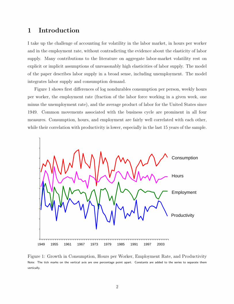
Figure 1 shows first differences of log nondurables consumption per person, weekly hours

per worker, the employment rate (fraction of the labor force working in a given week, one

minus the unemployment rate), and the average product of labor for the United States since

1949. Common movements associated with the business cycle are prominent in all four

measures. Consumption, hours, and employment are fairly well correlated with each other,

while their correlation with productivity is lower, especially in the last 15 years of the sample.

1949 1955 1961 1967 1973 1979 1985 1991 1997 2003

Consumption

Productivity

Employment

Hours

Figure 1: Growth in Consumption, Hours per Worker, Employment Rate, and ProductivityNote: The tick marks on the vertical axis are one percentage point apart. Constants are added to the series to separate them

vertically.

2

I take the driving force of the movements shown in the figure to be changes in the

marginal product of labor, arising from random changes in total factor productivity growth,

in the terms of trade, and in the prices of factors other than labor. I portray the movements

of hours per worker in terms of a standard labor supply schedule without extreme wage

elasticity.

Understanding the cyclical movements of consumption in this framework is a challenge.

With preferences additively separable in work and consumption, it is difficult to construct

a model on standard principles that generates a strong hours response—as seen in Figure

1—and a strong pro-cyclical consumption response. The approach I take is to invoke fairly

high complementarity between consumption and hours of work. High marginal productivity

induces households to substitute purchased consumption goods and services to replace the

diminished time at home resulting from longer hours of work.

The second big challenge is to understand the movements of the employment rate in this

framework. I do so by making job search an integral part of the model and a distinct use

of peoples’ time. In this area, the model draws on the Mortensen and Pissarides (1994)

theory of equilibrium unemployment. I develop an employment function that is in some

ways analogous to an hours supply function. But it does not depend solely on choices made

by workers. That is, job search is not just a use of time determined by individual choice in

response to a market wage. Rather, it is an equilibrium of interaction among jobseekers and

recruiting employers.

In broad summary, the model in this paper considers a worker in a family that maximizes

the expected discounted sum of future utility, which depends positively on the members’

levels of consumption and negatively on their hours of work. The worker has an hourly

marginal product w. I denote it w because it functions as the wage in the determination of

the worker’s hours. The family’s marginal utility of goods consumption, λ, set at the same

level for all members, describes the long-run or permanent level of well-being in the economy.

The marginal product w captures the deviation of current conditions from normal. When

w is higher than the level corresponding to current consumption, hours will be higher than

normal as workers take advantage of the temporarily exceptional benefit of working.

Given the state variables λ and w, hours of work per worker, h, is a function h(λ,w)

expressing the level that equates the marginal disutility of work to λw. Hours supply is

an increasing function of both λ and w. A companion function, ce(λ,w) describes the cor-

3

responding choice of consumption for employed family members. I view the increases in

consumption that occur when w is unusually high (that is, relative to λ) as resulting from

the positive response of consumption to w through the consumption-work complementar-

ity. In addition, the function cu(λ,w) describes the family’s choice of consumption for its

unemployed members—with consumption-hours complementarity, it will be lower than con-

sumption of the employed.

I consider a broad class of models where the employment rate is a function n(λ,w) of the

same two variables. The class includes the Mortensen and Pissarides (1994) (MP) model, the

basic statement of the theory of unemployment widely in use today. The employment rate

is an increasing function of both λ and w. Other members of the class of models differ from

the MP model by the principle governing the compensation paid to newly hired workers.

Some other members yield much higher responses of unemployment to the two driving forces

than is present in the MP model, but unemployment remains a function of the two driving

forces alone. Higher responses of unemployment are the result of more limited response of

compensation to driving forces. I note that the efficiency-wage model is a member of the

broader class—the efficiency-wage principle stabilizes compensation at the point needed to

prevent shirking.

In this paper, I do not consider the small procyclical movements of participation in the

labor force—Hall (forthcoming) documents these movements. The function

h(λ,w)n(λ,w). (1)

governs the total volatility of hours of work, apart from participation. When the marginal

product w rises temporarily above the level corresponding to λ, employment and hours rise,

creating a cyclical bulge in total hours per person. Recessions are times when the opposite

occurs.

I treat the state variables λ and w as unobserved latent variables. I take each of the four

indicators—consumption, hours, the employment rate, and productivity—as a function of the

two latent variables plus an idiosyncratic residual. The model falls short of identification.

I use information from extensive research on some of the coefficients to help identify the

remaining coefficients. I also use inequalities derived from the model to limit the ranges of

the coefficients. I embody the information in a prior distribution and compute the posterior

distribution of the parameters from the prior and the sample evidence shown in Figure 1.

The posterior distribution shows that the empirical employment function is much more

4

sensitive to λ and w than is its counterpart in the MP model. Although I treat this as an

empirical finding not associated with any specific theory of compensation determination, it

implies that compensation paid to newly hired workers is stickier than it would be with Nash

bargaining—unemployment rises in recessions because the marginal product of labor falls

relative to the compensation paid to newly hired workers, so employers cut their job-creation

efforts.

The model provides an internally consistent account of cyclical movements in the labor

market. It attains the goal of explaining the large observed cyclical volatility of labor input

without invoking an unrealistically high elasticity of labor supply. The main way that it

attains the goal is to explain the movements of unemployment as responses to the two

driving forces. Because most of the decline in labor input that occurs in a recession takes

the form of rising unemployment rather than reduced hours of those at work, the shift in

emphasis from the elasticity of labor supply to the elasticity of unemployment is appropriate.

This paper makes progress on the issues in Hall (1997). That paper had a similar factor

structure to this one, but did not include unemployment. It found unexplained movements

in total labor input that it labeled shifts in preferences. This paper interprets the same

movements as the result of changes in equilibrium unemployment and succeeds in matching

the observed data without invoking any shifts in preferences.

2 Insurance

The analysis in this paper makes the assumption that workers are insured against the per-

sonal risk of the labor market and that the insurance is actuarially fair. The insurance

makes payments based on outcomes outside the control of the worker that keep all workers’

marginal utility of consumption the same. This assumption—dating at least back to Merz

(1995)—results in enormous analytical simplification. In particular, it makes the Frisch sys-

tem of consumption demand and labor supply the ideal analytical framework. Absent the

assumption, the model is an approximation based on aggregating employed and unemployed

individuals, each with a personal state variable, wealth.

I do not believe that, in the U.S. economy, consumption during unemployment behaves

literally according to the model with full insurance against unemployment risk. But fam-

ilies and friends may provide partial insurance. I view the fully insured case as a good

and convenient approximation to the more complicated reality, where workers use savings

5

and partial insurance to keep consumption close to the levels that would maintain roughly

constant marginal utility. See Hall (2006) for evidence supporting the view that the fully

insured case is a good approximation for the response of workers to unemployment. I make

no claim that workers are insured against idiosyncratic permanent changes in their earnings

capacities, only that the transitory effects of unemployment can usefully be analyzed under

the assumption of insurance.

3 Dynamic Labor-Market Equilibrium

I now consider an economy with many identical families, each with a large number of mem-

bers. All workers face the same pay schedule and all members of all families have the same

preferences. The family insures its members against personal (but not aggregate) risks and

satisfies the Borch-Arrow condition for optimal insurance of equal marginal utility across

individuals. In each family, a fraction nt of workers are employed and the remaining 1− ntare searching. These fractions are outside the control of the family—they are features of

the labor market. In my calibration, a family never allocates any of its members to pure

leisure—it achieves higher family welfare by assigning all non-working members job search

and it never terminates the work of an employed member. Thus, as I noted earlier, I ne-

glect the small variations in labor-force participation that occur in the actual U.S. economy.

To generate realistically small movements of participation in the model I would need to

introduce heterogeneity in preferences or earning powers.

This section develops a model that generalizes the canonical model of Mortensen and

Pissarides (1994). I adopt the undirected search and matching functions of their model, but

replace the Nash bargain with a more general characterization of the determination of a

newly hired worker’s compensation. I also follow other authors in generalizing preferences

and incorporating choice over hours of work. I will refer to the result as the extended MP

model.

3.1 Search and matching

Employers post vacancies. Each period, the probability that a worker will become avail-

able to fill the vacancy is q. In tighter labor markets, vacancies are harder to fill and q is

lower. The MP model characterizes the tightness of the labor market in terms of the va-

cancy/unemployment ratio θ. The job-finding rate is an increasing and concave function φ(θ)

6

and the vacancy-filling rate is the decreasing function φ(θ)/θ. The model assumes a constant

exogenous rate of job destruction, s. Employment follows a two-state Markoff process with

stochastic equilibrium

n =φ(θ)

s+ φ(θ). (2)

Because the job-finding rate φ(θ) is high—more that 25 percent per month—the dynamics

of unemployment are rapid. Essentially nothing is lost by thinking about unemployment as

if it were at its stochastic equilibrium and treating it as a jump variable. I will adopt this

convention in the rest of the paper. I invert equation (2) to find θ(n) and take the job-filling

probability to be the decreasing function

q(n) = φ(θ(n))/θ(n). (3)

In a tighter labor market with higher employment rate n, the job-filling rate q(n) is lower.

As in the MP model, employers incur a cost γ at the beginning of a period to maintain

a vacancy for the period, with probability q(n) of filling the job at the end of the period.

3.2 The employment contract

Employers pay workers wt for each hour of work in period t. Employers collect an amount

yt from a new worker. Both workers and employers are price-takers with respect to wt, so

the employment contract embodies efficient two-part pricing. I discuss the determination

of yt shortly; it is a key feature of the model. For simplicity I develop the model as if yt

were collected at the beginning of the period, but the results would be identical if it were

spread over the period of employment and yt were the present value as of the beginning of

the period of the amount deducted from wtht by the employer.

3.3 Production and the firm’s decisions

The economy has a single kind of output, with production function

F (Ht, Kt, ηt). (4)

Here Ht = ntht is total hours of work, Kt is the capital stock, and η is a vector of random

disturbances.

Firms make three decisions: (1) the number of vacancies to try to fill each period, (2)

the hours to demand from the existing work force, and (3) the demand for capital.

7

(1) Under the standard employment contract, firms exactly break even from employing a

new worker during the worker’s tenure. They decide whether to recruit workers based upon

the immediate payoff,

q(nt)yt − γ. (5)

They invest γ in holding a vacancy open for the period and have a probability q(nt) of

gaining the payoff yt. Firms are large enough to absorb the fully diversifiable risk associated

with the probability of successful recruiting. Firms would create infinitely many vacancies

if the payoff were positive and zero if it were negative. Equilibrium requires that the payoff

to recruiting be zero:

q(n)y = γ. (6)

The employment rate that solves this zero-profit condition is a function n(y), which I call

the employment function.

(2) The number of employees at a firm is a state variable. The first-order condition,

∂F (nh,K)

∂H= wt, (7)

describes the firm’s demand for their hours.

(3) A capital services market allocates the available capital efficiently among firms in

proportion to their employment levels. The first-order condition,

∂F (nh,K)

∂K= rt, (8)

describes the firm’s demand for capital.

3.4 The family’s decisions

As in most research on choices over time, I assume that preferences are time-separable,

though I am mindful of Browning, Deaton and Irish’s (1985) admonition that “the fact

that additivity is an almost universal assumption in work on intertemporal choice does not

suggest that it is innocuous.” In particular, additivity fails in the case of habit.

The family orders levels of hours of employed members, ht, consumption of employed

members, ce,t, and consumption of unemployed members, cu,t, within a period by the utility

function,

ntU(ce,t, ht) + (1− nt)U(cu,t, 0) (9)

8

The family orders future uncertain paths by expected utility with discount factor δ. The

family solves the dynamic program,

V (Wt, ηt) = maxht,ce,t,cu,t

ntU(ce,t, ht) + (1− nt)U(cu,t, 0)+

E δV ((1 + rt)[Wt − ntce,t − (1− nt)cu,t]− φ(nt)(1− nt)yt + wtntht, ηt+1) (10)

Here V (Wt, ηt) is the family’s expected utility as of the beginning of period t and Wt is wealth.

The expectation is over the conditional distribution of ηt+1. The amount φ(nt)(1−nt) is the

flow of new hires of family members, each of which costs the family yt.

The family utility function may serve as a reduced form for a more complicated model

of family activities that includes home production.

3.5 Equilibrium

Let η(t) be the history of the random driving forces up to time t. An equilibrium in this

economy is a wage function w(η(t)), a return function r(η(t)), and an employment rate function

nt(η(t)) such that the supply of hours h(η(t)) and the supply of savings, W (η(t)), from the

family’s maximizing program in equation (10) equal the firm’s demands from equations (7)

and (8), and the recruiting profit in equation (5) is zero, for every η(t) in its support.

3.6 State variables

I let λt be the marginal utility of wealth (and also marginal utility of consumption):

λt =∂V

∂Wt

= δ(1 + rt) E∂V

∂Wt+1

(11)

I take λt and the hourly wage wt as the state variables of the economy relevant to labor-

market equilibrium. Both state variables are complicated functions of the underlying driving

forces η. In particular, λt embodies the entire forward-looking optimization of the household

based on its perceptions of future earnings.

3.7 Hours, consumption, and employment

The family’s first-order conditions for hours and the consumption levels of employed and

unemployed members are are:

Uh(ce,t, ht) = −λtwt (12)

9

Uc(ce,t, ht) = λt (13)

Uc(cu,t, 0) = λt (14)

These conditions define three functions, ce(λt, wt), h(λt, wt), and cu(λt) giving the consump-

tion and hours of the employed and the consumption of the unemployed. With consumption-

hours complementarity, cu < ce.

3.8 The compensation bargain

I am agnostic about the principles underlying the bargain—the only restriction is that the

bargained payment is a function y(λ,w) of the two state variables. One could interpret this

assumption as a Markoff property, the exclusion of any other endogenous state variable aris-

ing from the bargaining game between worker and employer. This exclusion has substance,

as it rules out a state variable that might capture the inertia of compensation. In the setup

of this paper, compensation can be sticky in the sense of being unresponsive to the state

of the labor market, but it cannot be sticky in the sense of being under the influence of a

slow-moving state variable other than λ and w. A bargaining theory that implies an endoge-

nous state variable that imparts inertia to compensation would be an exciting addition to

the post-MP literature, but it has yet to be developed.

I note that the Nash wage bargain is a member of the class of models where y is a

function of the two state variables alone. The reservation payment for the employer, having

encountered a worker, is zero—the employer is indifferent to hiring at that point and comes

out definitely ahead if the worker makes any positive payment. The family’s upper limit on

the payment is the amount of the increase in its value function from shifting a member from

unemployment to unemployment. From equation (10), that amount is

U(ce, h)− U(cu, 0) + λ(−ce + cu + wtht) (15)

in utility terms. This is the change in utility when a member moves from unemployment to

employment (a negative amount) plus the budgetary effect of the increase in consumption

spending (a negative consideration) plus the added earnings. In terms of purchasing power,

the reservation payment is

R(λ,w) =U(ce, h)− U(cu, 0)

λ− ce + cu + wtht. (16)

10

All of the terms in this expression are functions of λ or w or both. Let the Nash bargaining

weight of the job-seeker be ν. The Nash-bargain upfront payment is y(λ,w) = (1−ν)R(λ,w).

The employment function n(y(λt, wt)) can now be written n(λt, wt), so it joins consump-

tion and hours as functions of the two state variables, a property I will exploit shortly in the

empirical analysis.

3.9 Volatility

Volatility in the labor market occurs because of movements in the wage w(η(t)), arising from

the shifts in technology that ηt induces. These could be changes in productivity or in other

factors that appear in the technology as a reduced form, such as changes in the terms of

trade. The volatility of hours operates in the standard way—an increase in the wage raises

h(λ,w) through the direct effect of w but the resulting decline in λ, arising from the favorable

effect of a higher wage on wealth, lowers hours. Most volatility in the U.S. economy comes

from variations in the employment rate n(λ,w). Here again a higher wage raises employment

while the resulting higher wealth and lower value of λ lowers employment, but, according to

the evidence in this paper, employment is more sensitive to both variables than is the supply

of hours.

The response of the employment rate to changes in the driving forces depends directly

on the payment y(λ,w) that a newly hired worker makes to the employer—see equation

(6). The higher this payment, the tighter is the labor market, because employers recruit

new workers more aggressively when the payoff is higher. If the payment were fixed, the

employment rate would also be fixed. In fact, when the driving forces raise the wage w, the

employment rate rises, according to the evidence later in this paper. So an increase in the

wage induces an increase in the upfront payment, y. Because the payment is a deduction

from the worker’s total compensation, the positive response of the payment to w means that

compensation does not rise in proportion to the wage—it is sticky in that sense. If, as seems

likely, the upfront payment is amortized over the duration of a job, then the elasticity of the

compensation that workers receive with respect to the underlying wage w is less than one.

A higher w delivers more value from the employment relation to the employer and induces

greater recruiting effort and thus a tighter labor market with a higher employment rate n.

In this framework, I interpret Shimer (2005) as showing that the value of the upfront

payment y resulting from a Nash bargain with roughly equal bargaining weights has low

11

sensitivity to w and results in low volatility of the employment rate. At the other extreme, if

compensation to the worker—the present value of wh over the job less the upfront payment

y—were unresponsive to w, y would move in proportion to w. In this situation of completely

sticky compensation, recruiting effort would rise sharply with w and the volatility of the

employment rate would be high and procyclical. The finding of this paper, that the employ-

ment rate is quite sensitive to w, implies that newly hired workers let employers keep some

important part of an increase in w because the worker makes a higher upfront payment y.

In general, the finding of sensitivity of n(λ,w) to w implies some stickiness of compensation.

3.10 Models within the framework of this paper

Hall and Milgrom (forthcoming) develop an alternating-offer bargaining model and cali-

bration in which compensation is sufficiently insensitive to labor-market conditions that

productivity changes cause realistic changes in unemployment. Hagedorn and Manovskii

(forthcoming) generate similar responses with Nash bargaining by assuming low bargaining

power for the worker and high elasticity of labor supply.

The efficiency-wage model of unemployment volatility, as developed by Alexopoulos

(2004) also fits within the framework developed above. Her model omits explicit treatment

of the search and matching process, but the substance is the same. Under the efficiency-wage

principle, employers set compensation at the level needed to prevent short-run opportunism

among workers—their share of the employment surplus needs to be large enough to keep

them working effectively. When productivity rises, the benefits go mostly to employers, who

respond by recruiting harder and tightening the labor market.

3.11 The role of λ

The marginal utility of consumption, λ, enters the extended MP model by determining the

value of time at home in relation to the value of work. When λ is high, job-seekers are

more interested in finding work because they value time away from work less. Workers

have lower reservation levels of compensation as a result, and the compensation bargain is

more favorable to the employer. Thus employment is an increasing function of λ. See Hall

and Milgrom (forthcoming) for a discussion of the relation between the MP and related

models with full preferences (variable marginal rates of substitution between consumption

and hours) and the linear preferences that most of the MP literature assumes. In the model

12

with full preferences, λ plays the role of the fixed leisure premium z that Mortensen and

Pissarides and most of their followers assumed.

4 Unemployment Theories

What theories of employment and unemployment fit the paradigm of the extended MP

model, where the employment rate is a function of λ and w? I distinguish three broad

classes of theories.

First, the pure equilibrium model of employment launched by Rogerson (1988) places

workers at their points of indifference between work and non-work, so compensation just

offsets the disamenity of the loss of time at home. Labor supply is perfectly elastic at that

level of compensation. The employed are those who wind up in jobs at the labor demand

prevailing at that compensation.

Second, search-and-matching models—surveyed recently by Rogerson, Shimer and Wright

(2005)—divide the labor market into many sub-markets, each in equilibrium. Unemployment

arises because some workers are in markets where their marginal products do not cover the

disamenity of work. The canonical Mortensen and Pissarides (1994) model is a leading

example: Workers are either in autarky, unmatched with any employer, in which case they

have zero marginal product by assumption, or they are matched and are employed at a

marginal product above their indifference point. Job-seekers enjoy a capital gain upon finding

a job. Although most search-and-matching models assume fixity of hours, that assumption is

not essential and is straightforward to relax—Andolfatto (1996) was a pioneer on this point.

A key assumption of the MP model is that the firm’s demand for labor is perfectly elastic.

This assumption only makes sense if the labor market is at the point where the total supply

of hours equals the total demand for hours at the marginal product w.

Third, allocational sticky-wage models invoke a state variable, the sticky wage, that

controls the allocation of labor. Employers choose total labor input to set the marginal

product of labor to the sticky wage. In that case, the sticky wage is the marginal product,

w, as well. As far as I know, the literature lacks a detailed, rigorous account of the resulting

equilibrium in the labor market comparable to the MP model. One simple view is that

employed workers work h(λ,w) hours and that the number employed, n, is the total number

of hours demanded divided by h(λ,w). Unemployment of the rent-seeking type in Harris and

Todaro (1970) results whenever n falls short of the labor force. In that case, the unemployed

13

are those queued up for scarce jobs. The arguments of the employment function n(·) include

λ, w, and the other determinants of labor demand. But n depends negatively on λ because

a higher value results in more hours of work by the employed and thus fewer jobs. And n

depends negatively on w for a similar reason and because labor demand falls with w. Finally,

n depends on the other determinants of labor demand, such as the capital stock. Thus,

because they drop the key assumption of perfectly elastic labor demand, allocational sticky-

wage models have rather different implications for the employment function. In particular,

labor-market outcomes depend on more than the two variables λ and w.

In the class of models where employment depends just on λ and w, a value of w that is

high in relation to λ tightens the labor market and results in high employment. An important

implication of this property is that the response of unemployment to changes in w is stronger

when λ remains constant—a transitory change in w—than when the change is permanent

and λ changes as well. Pissarides (1987) made this point early in the development of the

MP literature, though without a full development of the underlying preferences. Blanchard

and Gali (2007) make the same point for the special case of separability between hours and

consumption, and with consumption entering as the log.

The equilibrium model plainly belongs to this class. In that model, labor supply is

perfectly elastic at a value of w dictated by λ. The employment function n(λ,w) is a

correspondence mapping the two variables into 1.0 if w is above the critical value, into the

unit interval at that value, and into zero below the value. On the other hand, allocational

sticky-wage models are not in the class because they require that employment shifts along

with the non-wage determinants of labor demand.

A quick summary of this discussion is that sticky-compensation models in the extended

MP class are consistent with the model in this paper, while sticky-wage models are not.

I will proceed on the assumption that a function n(λ,w) that gives the employment rate

n in an environment where marginal utility is λ and the marginal product is w is a reasonable

way to think about the employment rate. The next step is to measure the response of the

rate to the two determinants.

5 Research on Preferences

The empirical approach in this paper rests on using prior information about preferences from

research on individual behavior. This section relates the three functions h(λ,w), ce(λ,w),

14

and cu(λ) to that research.

Consider the standard intertemporal consumption-hours problem without unemploy-

ment,

max Et

∞∑τ=0

δτU(ct+τ , ht+τ ) (17)

subject to the budget constraint,

∞∑τ=0

(wt+τht+τ − pt+τct+τ ) = 0. (18)

Here pτ is the price of the consumption good. Both the wage wτ and the price pτ are quoted

in units of abstract purchasing power, as of time t—they are Arrow-Debreu prices.

I let C(λp, λw) be the Frisch consumption demand and H(λp, λw) be the Frisch supply

of hours per worker. See Browning, Deaton and Irish (1985) for a complete discussion of

Frisch systems in general. They satisfy, for consumption and hours at time zero,

Uc (C(λp0, λw0), H(λp0, λw0)) = λp0 (19)

and

Uh (C(λp0, λw0), H(λp0, λw0)) = −λw0 (20)

Here λ is the Lagrange multiplier for the budget constraint. Consumption in period t is

C(λtpt, λtwt) and similarly for hours. I will focus on time t and drop the time subscript in

what follows.

The Frisch functions have symmetric cross-price responses: C2 = −H1. They have three

basic first-order or slope properties:

• Intertemporal substitution in consumption, C1(λp, λw), the response of consumption to

changes in its price

• Frisch labor-supply response, H2(λp, λw), the response of hours to changes in the wage

• Consumption-hours cross effect, C2(λp, λw), the response of consumption to changes

in the wage (and the negative of the response of hours to the consumption price). The

expected property is that the cross effect is positive, implying substitutability between

consumption and hours of non-work or complementarity between consumption and

hours of work.

15

Each of these responses has generated a body of literature, which I will draw upon. In

addition, in the presence of uncertainty, the curvature of U controls risk aversion, the subject

of another literature.

Consumption and hours are Frisch complements if consumption rises when the wage

rises (work rises and non-work falls)—see Browning et al. (1985) for a discussion of the

relation between Frisch substitution and Slutsky-Hicks substitution. People consume more

when wages are high because they work more and consume less leisure. Browning et al.

(1985) show that the Hessian matrix of the Frisch demand functions is negative semi-definite.

Consequently, the derivatives satisfy the following constraint on the cross effect controlling

the strength of the complementarity:

C22 ≤ −C1H2. (21)

To understand the three basic properties of consumer-worker behavior listed earlier, I

draw primarily upon research at the household rather than the aggregate level. The first

property is risk aversion and intertemporal substitution in consumption. With additively

separable preferences across states and time periods, the coefficient of relative risk aversion

and the intertemporal elasticity of substitution are reciprocals of one another. But there

is no widely accepted definition of measure of substitution between pairs of commodities

when there are more than two of them. Chetty (2006) discusses two natural measures of

risk aversion when hours of work are also included in preferences. In one, hours are held

constant, while in the other, hours adjust when the random state becomes known. He notes

that risk aversion is always greater by the first measure than the second. The measures are

the same when consumption and hours are neither complements nor substitutes.

The Appendix summarizes the findings of recent research on the three key properties

of the Frisch consumption demand and labor supply system. The own-elasticities have

been studied extensively. The literature on measurement of the cross-elasticity is sparse,

but a substantial amount of research has been done on an equivalent issue, the decline in

consumption that occurs when a person moves from normal hours of work to zero because

of unemployment or retirement. I believe that a fair conclusion from the research is that a

person in the middle of the joint distribution of the three properties has a Frisch elasticity of

consumption demand of −0.5, a Frisch elasticity of hours supply of 0.9, and a Frisch cross-

elasticity of 0.3. I use informative priors for these parameters. I use much less informative

priors for parameters that have received less attention in past research—the elasticities of

16

the employment function with respect to λ and w, the variances of the stochastic elements,

and the correlation of λ and w.

To derive the relation between the Frisch functions and the corresponding functions used

in the extended MP model, I normalize the price as pt = 1. Thus in period t, values are

stated in terms of units of period-t output. Further, λt becomes marginal utility in period t

under this normalization. Then

c(λ,w) = C(λ, λw) (22)

and

h(λ,w) = H(λ, λw). (23)

Notice that the response of consumption to a change in marginal utility λ is:

c1 = C1 + wC2 (24)

and for hours:

h1 = −C2 + wH2. (25)

6 Latent Factor Model

Because the disturbances in the model stated in levels are nonstationary, I work in first

differences of logs, that is, rates of growth. I approximate the consumption demands, hours

supply, and employment functions as log-linear, with βc,c denoting the elasticity of consump-

tion with respect to its own price (the elasticity corresponding to the partial derivative c1

in the earlier discussion), βc,h the cross-elasticity of consumption demand and hours supply,

and βh,h the own-elasticity of hours supply. I further let βn,λ denote the elasticity of employ-

ment with respect to marginal utility λ and βn,w the elasticity with respect to the marginal

product w.

6.1 Hours and employment

The factor equation for hours is:

∆ log h = (−βc,h + βh,h)∆ log λ+ βh,h∆ logw + εh (26)

and for employment is:

∆ log n = βn,λ∆ log λ+ βn,w∆ logw + εn. (27)

17

Here βh,h and −βc,h are the Frisch own- and cross-elasticities of hours supply for employed

workers, βn,λ and βn,w are the elasticities of the employment function, and the εs are idiosyn-

cratic random components.

6.2 Consumption

The model disaggregates the population by the employed and unemployed, who consume ce

and cu respectively. Only average consumption c is observed. Observed consumption is the

average of the two levels, weighted by the employment and unemployment fractions:

c = nce + (1− n)cu. (28)

Taking first differences of the log-linearization in the variables, around the point n, ce, cu,

and c, I find

∆ log c =ce − cuc

n∆ log n+ ncec

∆ log ce + (1− n)cuc

∆ log cu. (29)

The consumption changes relate to latent factors as

∆ log ce = (βc,c + βc,h)∆ log λ+ βc,h∆ logw (30)

and

∆ log cu = βc,c∆ log λ. (31)

Substituting equations (30) and (31) into equation (29), I find, now including an idiosyncratic

disturbance εc,

∆ log c =ce − cuc

n∆ log n+ βc,c∆ log λ+ βc,hncec

(∆ logw + ∆ log λ) + εc. (32)

Finally, I substitute equation (27) for ∆ log n to get

∆ log c =

(βc,c + βc,h

cecn+ βn,λ

ce − cuc

n

)∆ log λ

+

(βc,h

cecn+ βn,w

ce − cuc

n

)∆ logw + εc +

ce − cuc

nεn. (33)

I use relatively recent data for the ratios cec

and cuc

. The accuracy of the log-linear

approximation rests on the constancy of these ratios over the sample period. The model

implies that an increase in w lowers λ more than in proportion—see Figure 2. Thus equations

(30) and (31) imply that the gap between ce and cu should close over time as w trends

18

upward. I do not incorporate this trend in the calculation for the following reason: The

model embodies a backward-bending uncompensated labor-supply function. In fact, hours

were fairly constant over the sample period. From the condition

Uc(cu, 0)

Uc(ce, h)= 1, (34)

it follows that with preferences where the marginal utility of consumption is homogeneous

of any degree, such as the non-separable preferences in Hall and Milgrom (forthcoming),

the ratio cu/ce remains constant if h remains constant. Thus the addition of any trend in

preferences, presumably reflecting a trend in home technology for which the preferences are

a reduced form, will deliver a constant cu/ce ratio at the same time that it delivers the right

trend in hours. The model as estimated ignores trends because it is based on the covariances

of the log first differences and does not consider the means.

6.3 Productivity

I measure productivity as the average product of labor, m = qh, where q is output per worker.

I let α be the elasticity of the production function with respect to labor input. From

w =∂F

∂H= α

q

h, (35)

I get the equation for the log-change in m:

∆ logm = ∆ logw −∆ logα. (36)

Notice that ∆ logα = 0 for a Cobb-Douglas technology. Finally, I define εm to include

−∆ logα and any other disturbances, such as measurement error, so the equation for m in

the model is

∆ logm = ∆ logw + εm. (37)

6.4 Intuition about estimation

Equation (37) suggests the use of ∆ log w = ∆ logm as the observed counterpart of the

latent factor ∆ logw. Given knowledge of the Frisch elasticity of hours supply, βh,h, and

of the cross-elasticity βc,h, data on hours provide an observable counterpart for the latent

factor ∆ log λ:

∆ log λ =1

βh,h − βc,h(∆ log h− βh,h∆ logw) (38)

19

Then, one could consider the coefficients from the regression of ∆ log n on ∆ log w and ∆ log λ

as estimates of the parameters βn,λ and βn,w. The procedure described in the next section is

a close cousin of this approach. It uses prior distributions on βh,h and βc,h, rather than taking

them as known, and it attends to the econometric issue of the correlation of the disturbance

in the estimating equation with the right-hand variables. But the basic approach is to infer

well-being, as measured by λ, from the observed choice of hours given the wage w, and then

to examine the response of the employment rate n to the two determinants, λ and w.

The regression of ∆ log c on ∆ log w and ∆ log λ would similarly provide estimates of the

compound coefficients of equation (33). The coefficient on ∆ log λ would estimate

βc,c + βc,hcecn+ βn,λ

ce − cuc

n. (39)

An estimate of βc,c could be extracted from this coefficient, because all the other elements

would be known at this stage. The coefficient on ∆ log w would estimate

βc,hcecn+ βn,w

ce − cuc

n. (40)

This coefficient involves no further unknown parameter, so it appears that its value could

help fix the values of the other parameters. But this appearance is false. The model is two

parameters short of identification, so in a classical setting, one would need to assume known

values for two of the parameters.

The estimation procedure I employ examines the response of consumption to the latent

value of ∆ log λ and interprets it as coming from three sources: (1) the direct substitution

response controlled by βc,c by the consumption of the employed and the unemployed, (2) the

cross effect controlled by βc,hcecn for the consumption of the employed only, and (3) the change

in consumption associated with the change in employment and the higher consumption of

the employed, controlled by βn,λce−cucn. Similarly, the estimation procedure interprets the

response of consumption to ∆ logw as coming from two sources: (1) the cross effect from the

wage on the consumption of the employed, controlled by βc,hcecn and (2) the consumption

change induced by employment change, controlled by βn,wce−cucn.

6.5 Statistical model

I assume that the idiosyncratic components, ε, are uncorrelated with λ and w. This assump-

tion is easiest to rationalize if the εs are measurement errors.

20

The model has 12 parameters: the 5 β slope coefficients, the variances and correlation of

the latent factors, σ2λ, σ

2w, and σλ,w, and the variances of the four idiosyncratic components,

σ2ε,c, σ

2ε,h, σ

2ε,n, and σ2

ε,m. The model implies 10 observed moments, the distinct elements of the

covariance matrix of the observables, the employment-adjusted log-change in consumption

and the log-changes of hours, employment, and productivity. It is further restricted by

non-negativity of the 6 variances, by the Cauchy inequality for the covariance,

σ2λ,w ≤ σ2

λσ2w, (41)

and by the concavity condition, equation (21).

Under the assumption that the random variables λ, w, εc, εh, εn, and εm are multivariate

normal, any parameter set that matches the sample moments achieves the maximum of the

likelihood function. The likelihood has a plateau of equal height for any set of parameters

with this property. The posterior distribution is governed by the prior everywhere on the

plateau. Stripped of an inessential constant, the log-likelihood function is

−T2

[log det Ω + tr

(Ω−1Ω

)]. (42)

Ω is the covariance matrix of the observables implied by the model and Ω is the sample

covariance matrix. On the plateau, Ω = Ω and the value of the log-likelihood is

−T2

(log det Ω + 4

). (43)

The prior distribution is discrete. It takes the 12 parameters to be independent of one

another. The marginal distribution of each parameter takes on equal values at four equally

spaced points. Thus the posterior distribution is defined on a lattice of 412 = 16.8 million

points. I calculate the exact marginals of the posterior distribution by summation over these

points.

6.6 Inferring the values of λ and w

I write the model in matrix form as

∆x = θλ∆ log λ+ θw∆ logw + ε. (44)

Here x is the vector of observed values of the logs of consumption, hours, employment, and

productivity. I infer λ as a linear combination, λ = a′x. I choose the weights a as the

coefficients of the projection of λ on x, using the moments implied by the parameter values

at the posterior mean. I calculate the inference of w, w, similarly.

21

Parameter Interpretation Mean Loweest value Highest value

β c,cFrisch own-price elasticity of consumption -0.50 -0.6 -0.4

β c,hFrisch cross-price elasticity of consumption 0.30 0.0 0.6

β h,hFrisch wage elasticity of hours 0.90 0.8 1.0

β n,λElasticity of employment with respect to λ 0.50 0.0 1.0

β n,wElasticity of employment with respect to w 1.00 0.0 2.0

σ2λ Variance of latent λ 2.15 0.3 4.0

σ2w Variance of latent w 2.15 0.3 4.0

ρ Correlation of λ and w -0.70 -0.9 -0.5

σ2c

Variance of consumption noise 1.00 0.5 1.5

σ2h Variance of hours noise 0.30 0.2 0.4

σ2n

Variance of employment noise 0.25 0.1 0.4

σ2m

Variance of productivity noise 0.75 0.3 1.2

Table 1: Priors

7 Prior Distributions

Table 1 shows the marginal prior distributions I use for the parameters. They are four-point

distributions for all parameters. The priors are highly informative when drawn from the

research summarized in Appendix A. They are less informative for parameters where earlier

work is either sparse or nonexistent, for the variances of the random elements, and for the

correlation of ∆ log λ and ∆ logw. I constrain the cross-elasticity βc,h to satisfy concavity

and the correlation of the latent factors to be greater than −1.

The ratio of unemployment consumption cu to employment consumption ce reflects the

same properties of preferences as does the Frisch cross-elasticity, βc,h. Accordingly, I take the

22

joint prior for the two parameters to have perfect correlation, with cu/ce = 0.75βc,w. The pro-

portionality factor 0.75 is derived from a parametric utility function that matches the means

of the priors of the Frisch elasticities—when the cross-elasticity is 0.20, the consumption

ratio is 0.85.

8 Data

To avoid complexities from durables purchases and measurement error in the consumption

of services, I use nondurables consumption as an indicator of consumption. I take the

quantity index for nondurables consumption from Table 1.1.3 of the U.S. National Income

and Product Accounts and population from Table 2.1. I take weekly hours per worker

from series LNU02033120, Bureau of Labor Statistics, Current Population Survey, and the

unemployment rate from series LNS14000000. I measure productivity as output per hour

of all persons, private business, BLS series PRS84006093. For further discussion of the

labor-market data, see Hall (forthcoming).

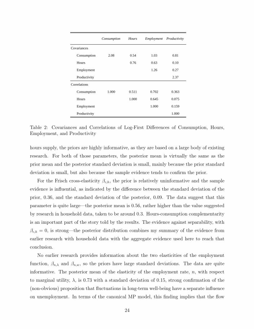
Table 2 shows the covariance and correlation matrixes of the log-differences of the four

series. Consumption is correlated positively with both hours and employment—it is quite

pro-cyclical. Consumption-hours complementarity can explain this fact. Not surprisingly,

hours and employment are quite positively correlated. Consumption has surprisingly high

volatility, a property not explained in this paper. Consumption also has by far the highest

correlation with productivity.

The variance of the employment rate is about 70 percent higher than the variance of

hours—the most important source for the added total hours of work in an expansion is the

reduction in unemployment. Hours and the employment rate are not very correlated with

productivity.

9 Results

Table 3 shows the means and standard deviations of the marginal prior and posterior distri-

butions of the 12 parameters of the model. In general, the decline in the standard deviation

from prior to posterior measures the information contributed by the sample evidence and

the difference between the prior and posterior means indicates the direction of the influence

of the evidence. For two key parameters, the Frisch own-elasticities of consumption and

23

Consumption Hours Employment Productivity

Covariances

Consumption 2.08 0.54 1.03 0.81

Hours 0.76 0.63 0.10

Employment 1.26 0.27

Productivity 2.37

Correlations

Consumption 1.000 0.511 0.702 0.363

Hours 1.000 0.645 0.075

Employment 1.000 0.159

Productivity 1.000

Table 2: Covariances and Correlations of Log-First Differences of Consumption, Hours,Employment, and Productivity

hours supply, the priors are highly informative, as they are based on a large body of existing

research. For both of those parameters, the posterior mean is virtually the same as the

prior mean and the posterior standard deviation is small, mainly because the prior standard

deviation is small, but also because the sample evidence tends to confirm the prior.

For the Frisch cross-elasticity βc,h, the prior is relatively uninformative and the sample

evidence is influential, as indicated by the difference between the standard deviation of the

prior, 0.36, and the standard deviation of the posterior, 0.09. The data suggest that this

parameter is quite large—the posterior mean is 0.56, rather higher than the value suggested

by research in household data, taken to be around 0.3. Hours-consumption complementarity

is an important part of the story told by the results. The evidence against separability, with

βc,h = 0, is strong—the posterior distribution combines my summary of the evidence from

earlier research with household data with the aggregate evidence used here to reach that

conclusion.

No earlier research provides information about the two elasticities of the employment

function, βn,λ and βn,w, so the priors have large standard deviations. The data are quite

informative. The posterior mean of the elasticity of the employment rate, n, with respect

to marginal utility, λ, is 0.73 with a standard deviation of 0.15, strong confirmation of the

(non-obvious) proposition that fluctuations in long-term well-being have a separate influence

on unemployment. In terms of the canonical MP model, this finding implies that the flow

24

Parameter Interpretation Prior meanPrior

standard deviation

Posterior mean

Posterior standard deviation

β c,cFrisch own-price elasticity of consumption -0.50 0.12 -0.49 0.07

β c,hFrisch cross-price elasticity of consumption 0.30 0.36 0.53 0.09

β h,hFrisch wage elasticity of hours 0.90 0.12 0.95 0.06

β n,λElasticity of employment with respect to λ 0.50 0.61 0.73 0.15

β n,wElasticity of employment with respect to w 1.00 1.21 1.60 0.33

σ2λ Variance of latent λ 2.15 2.24 3.58 0.72

σ2w Variance of latent w 2.15 2.24 1.14 0.57

ρ Correlation of λ and w -0.70 0.24 -0.72 0.13

σ2c

Variance of consumption noise 1.00 0.61 1.18 0.23

σ2h Variance of hours noise 0.30 0.12 0.35 0.05

σ2n

Variance of employment noise 0.25 0.18 0.25 0.11

σ2m

Variance of productivity noise 0.75 0.55 1.15 0.12

Table 3: Posterior Distribution

25

λ w

Consumption 0.31 1.13

Hours 0.42 0.95

Employment 0.73 1.60

Average product of labor 0.00 1.00

Table 4: Coefficients for Log-First Differences of Consumption, Hours, Employment, andProductivity on λ and w

benefit of not working, usually called z, is not a fixed parameter but rather an endogenous

variable. The posterior mean of the elasticity of n with respect to the marginal product of

labor, w, is 1.60 with a standard deviation of 0.33. All models in the MP tradition agree

that the employment rate responds positively to w, though they disagree on the magnitude.

The data appear to compel the view that the response is quite strong.

The priors are uninformative about the six variance parameters. These are stated as

variances of percentage changes (100 times log changes) of the variables. The data are

moderately successful in pinning down the variances of the two latent factors, λ and w, and

quite successful for the four variances of the noise components of the observed variables. The

prior on the correlation of the two latent factors favors a strong negative correlation of −0.7

and that data concur, so that the posterior mean is −0.72 with a standard deviation of 0.13

Table 4 shows the coefficients relating the observed variables to the latent variables λ

and w at the posterior means of the parameters. The coefficients for employment and for

the response of hours to w are the elasticities reported in Table 3 and those for productivity

are zero on λ and one on w. The more complicated relations are for consumption and for

the response of hours to λ, from equations (26) and (29).

The biggest surprise in Table 4 is the positive response of consumption to marginal utility

λ. Although one might think that marginal utility is a declining function of consumption,

theory does not require that property in a Frisch demand system. Recall from equation (29)

that the coefficient on λ in the consumption equation is

βc,c + βc,hcecn+ βn,λ

ce − cuc

n. (45)

The theoretical limit on the complementarity effect is, from equation (21),

βc,h ≤√−βc,cβn,w. (46)

26

From Table 3, the cross-elasticity is 0.53 while the square root is 0.68, comfortably larger.

The key point is that the coefficient of consumption on λ is not the own-price effect, which

is necessarily negative, but the own-price plus the cross-price effect, which can be positive if

complementarity is strong enough. Because of the aggregation of consumption across workers

and the unemployed, the complementarity effect has two components in equation (45). First,

a higher λ (lower well-being) raises the consumption of workers through the direct effect of

the complementarity, controlled by βc,h. Second, a higher λ increases the employment rate.

Because the employed consume more than the unemployed, average consumption rises on

this account as well. The second effect is controlled by βn,λ, whose posterior mean is 0.73.

Complementarity also explains the high response of consumption to the current marginal

product of labor, w. Again from equation (29), this response is

βc,hcecn+ βn,w

ce − cuc

n. (47)

The second term describes the stimulus to employment (decline in unemployment) that

accompanies an increase in w. The direct effect through βc,h is 0.53. The effect from

employment change is βn,w = 1.60 multiplied by the consumption-difference effect, which is

0.32.

The effect of λ on hours, 0.42, is correspondingly weak. The coefficient is −βc,h + βh,h.

Complementarity enters negatively, offsetting the relatively strong own-elasticity effect. An

increase in λ raises the price of consumption as it raises the reward to work. Because non-

work time is a substitute for consumption, people shift toward non-work when the price of

consumption rises.

The cross-elasticity βc,h plays an important role in explaining two features of the data

shown in Table 3—the generally high correlation of consumption with other cyclical vari-

ables and the particularly high correlation, relative to the hours and employment, between

consumption and productivity. Recall that productivity reveals the latent marginal product

w except for its own noise.

The sample evidence is also influential about the elasticities of employment with respect

to λ and w, a subject not previously investigated. The posterior reaches a sharp peak for the

w-elasticity at 1.4. Despite the model’s lack of identification and the uninformative priors

placed on these parameters (uniform from 0 to 1 for the first and from 0 to 2 for the second),

the other priors combine with the sample evidence to provide useful information.

27

Inferred λ Inferred w

Consumption -0.29 0.18

Hours 0.15 0.10

Employment 0.60 0.14

Average product of labor -0.76 0.37

Table 5: Coefficients for Inference of λ and w from Log-First Differences of Consumption,Hours, Employment, and Productivity

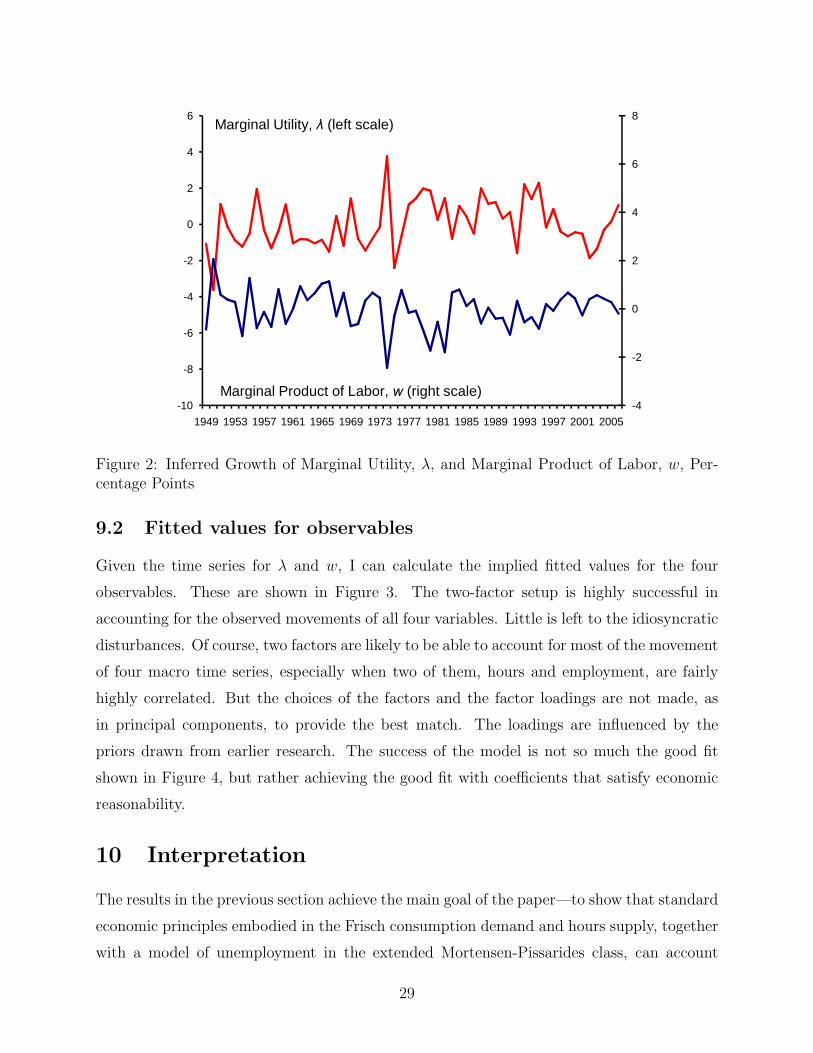
9.1 Implied values of marginal utility and marginal product

Table 5 shows the coefficients of the projection of the latent factors on the observed variables,

at the posterior means of the parameter values. As expected, the inference of marginal

utility puts negative weights on consumption and productivity—increases in them signal

improvements in well-being and thus lower values of marginal utility, λ. The inference puts

a positive weight on employment. The reason is shown in Table 4. An increase in λ raises

employment by more than it raises consumption and hours, relative to the coefficients for

w. Therefore, on the average, an increase in employment signals that an increase in λ has

occurred. The other feature of Table 5 worth noting is that the weight on productivity in

the inference of w is 0.37, well below the loading of productivity on w of 1. This finding

reflects the noise in productivity. The inference puts weight on all of the variables positively

correlated with productivity to filter out as much noise as it can.

Figure 2 shows the estimates of the change in marginal utility, ∆ log λ, and in the marginal

product, ∆ logw, resulting from the application of the coefficients in Table 5 to the data

on the four observables. The figure shows a pronounced negative correlation between the

changes in marginal utility and in the marginal product of labor. News that raises the

current marginal product of labor tends to raise lifetime well-being and thus to lower λ. If the

economy were perturbed by a single shock and households had no advance information about

the shock, the correlation would be −1. With multiple shocks and advance information, the

correlation would be less negative, in accord with the estimated correlation of −0.72.

28

-4

-2

0

2

4

6

8

-10

-8

-6

-4

-2

0

2

4

6

1949 1953 1957 1961 1965 1969 1973 1977 1981 1985 1989 1993 1997 2001 2005

Marginal Product of Labor, w (right scale)

Marginal Utility, λ (left scale)

Figure 2: Inferred Growth of Marginal Utility, λ, and Marginal Product of Labor, w, Per-centage Points

9.2 Fitted values for observables

Given the time series for λ and w, I can calculate the implied fitted values for the four

observables. These are shown in Figure 3. The two-factor setup is highly successful in

accounting for the observed movements of all four variables. Little is left to the idiosyncratic

disturbances. Of course, two factors are likely to be able to account for most of the movement

of four macro time series, especially when two of them, hours and employment, are fairly

highly correlated. But the choices of the factors and the factor loadings are not made, as

in principal components, to provide the best match. The loadings are influenced by the

priors drawn from earlier research. The success of the model is not so much the good fit

shown in Figure 4, but rather achieving the good fit with coefficients that satisfy economic

reasonability.

10 Interpretation

The results in the previous section achieve the main goal of the paper—to show that standard

economic principles embodied in the Frisch consumption demand and hours supply, together

with a model of unemployment in the extended Mortensen-Pissarides class, can account

29

-5

-4

-3

-2

-1

0

1

2

3

4

1949 1953 1957 1961 1965 1969 1973 1977 1981 1985 1989 1993 1997 2001 2005

ConsumptionFitted consumption

-3

-2

-1

0

1

2

3

1949 1953 1957 1961 1965 1969 1973 1977 1981 1985 1989 1993 1997 2001 2005

HoursFitted hours

-4

-3

-2

-1

0

1

2

3

1949 1953 1957 1961 1965 1969 1973 1977 1981 1985 1989 1993 1997 2001 2005

EmploymentFitted employment

-6

-4

-2

0

2

4

6

1949 1953 1957 1961 1965 1969 1973 1977 1981 1985 1989 1993 1997 2001 2005

ProductivityFitted productivity

Figure 3: Actual and Fitted Values of the Four Observables

30

for the higher-frequency movements of those variables. The accounting does not rest on

implausible values of any parameters. Most importantly, it does not rest on exaggerated

ideas about the elasticity of hours supply. Because the business cycle dominates the higher-

frequency movements of the variables, the results give a coherent account of the business

cycle.

The main way that the model escapes reliance on unrealistic elasticity of hours supply is

to recognize that the primary dimension of fluctuations in labor input at higher frequencies

is in the employment rate. Research on labor supply in household data does not reveal the

elasticities of employment, which are not features of household choice alone, but reflect an

equilibrium involving employer actions as well. This paper is the first to provide estimates

of an employment function of the type implied by the MP model, though one could interpret

Hagedorn and Manovskii (forthcoming) in terms of its implications for the employment

function. However, their approach rests on preferences that imply an extremely high wage

elasticity of hours supply.

Thus the centerpiece of the account in this paper of movements in labor input over the

cycle is the high elasticity of employment with respect to the marginal product of labor.

Employment falls and unemployment rises in a contraction because w falls and the elasticity

of employment with respect to w is something like 1.6. A rise in marginal utility offsets some

of the decline in w in the typical recession, but its elasticity is only around 0.7.

Recent research in the MP tradition has focused on the finding in Shimer (2005) that

an MP model with Nash bargaining and a reasonable set of parameter values cannot come

close to generating realistic fluctuations in unemployment from the observed movements in

productivity. In the vocabulary of this paper, the Nash bargain makes y virtually constant,

so equation (5) implies that the employment rate n is also virtually constant. Many papers

stimulated by Shimer’s work make specific changes, such as adding on-the-job search, to raise

the response of labor-market tightness to productivity. The approach here is different. I do

not take a stand on the source of the high elasticity of the employment function with respect

to w. In particular, I do not sponsor any particular bargaining principle in place of the

Nash bargain. I take a purely empirical approach to the measurement of the elasticity. In a

model that follows Mortensen and Pissarides in every respect except bargaining, my results

imply that bargaining power shifts toward workers during recessions, or, to put it differently,

that compensation is sticky. The upfront payment y falls when w falls, so compensation

31

is cushioned and does not fall as much. Because I take a purely empirical approach, there

is nothing surprising or significant in itself in the model’s ability to track variations in the

employment rate or other measures of tightness.

The primary focus of this paper is the demonstration of the consistency of a model

grounded in the theory of household behavior and in the MP class of unemployment theory

with the actual behavior of the key variables in the U.S. economy. The paper does not claim

to reject other theories. What the model interprets as high complementarity of hours and

consumption could arise from liquidity constraints that link current earnings to consumption

more tightly than under the assumptions made here. Less-than-full insurance against the

idiosyncratic risk of unemployment may contribute to the finding of high complementar-

ity as well. With respect to unemployment, I noted earlier that the assumption that the

determinants of the employment-payment bargain, y, are limited to those that are payoff-

relevant, while often made in game-theoretic models, is not completely compelling. Until

theory provides more guidance, it is hard to see how to characterize additional determinants

of y and test for their exclusion. On the other hand, the evidence here of the positive effect

of productivity on employment is inconsistent with the allocational sticky-wage model. This

finding rests on my econometric identifying assumptions. Under an alternative identification

strategy, as in Gali (1999), the effect of an innovation in productivity on employment is

negative and therefore consistent with the allocational sticky-wage model. The debate on

that topic remains unresolved.

11 Observable Variables Not Included in the Model

11.1 Compensation

The factor model does not consider the actual value of compensation paid to workers, de-

spite the key role of compensation in the Mortensen-Pissarides class of employment models.

In that class of models, compensation gains its influence over unemployment through the

non-contractible, pre-match effort of employers in attracting workers. These efforts—which

take the form of the creation of vacancies in the model—govern the tightness of the labor

market and thus the unemployment rate. The difference between the marginal product and

compensation, anticipated at the time of hiring, governs the employer’s vacancy-creation

efforts. The class of models has no further implications about the pattern of payment of

compensation over the period of employment. The bargained level of compensation has no

32

allocational role once a job-seeker and an employer find each other—it only divides the sur-

plus from the match. In particular, nothing rules out smoothing of compensation in relation

to productivity. I am not aware of any way to introduce observed compensation, averaged

over workers hired over the past 40 years, into the factor model without making special as-

sumptions about the determination of compensation during the period of employment. Even

if compensation is the result of period-by-period bargaining, one would have to take a stand

on bargaining principles to pin down compensation.

11.2 Asset returns

Equation (11) implies:

δ(1 + rt) Eλt+1

λt= 1, (48)

the asset-pricing condition of the consumption capital-asset pricing model. If the economy

traded an asset with a stochastic return, its return ratio would be inside the expectation.

In principle, this joint relation of asset returns would help pin down the latent variable,

∆ log λt. I tested this idea in a standard way, with the equation,

E δλt+1

λtrx,t = 0, (49)

where rx,t is the excess return of the S&P 500 stock portfolio over one-year Treasury bills.

The average value of rx,t is the equity premium and is 6.6 percent per year over the period I

used (1953 to 2003), with a standard error of 2.5 percent. The average value of the compound

random variable λt+1

λtrx,t over the same period is the same, 6.6 with a standard error of 2.5.

The t-statistic for the hypothesis that the value is zero, as required by asset-pricing theory,

is 2.6, indicating strong rejection. This finding replicates the famous conclusion of Mehra

and Prescott (1985). Campbell and Cochrane (1999) discuss the challenge of constructing a

successful asset-pricing variable out of aggregate consumption. The variable needs to have

vastly higher volatility than would any marginal utility based on standard principles and

reasonable risk aversion.

The alterations I have introduced in this paper to measure λ that make it differ from

Mehra and Prescott’s simple calculation from standard preferences do not result in anything

like the highly volatile variable needed to satisfy the asset-pricing condition for the equity

premium or for other asset-pricing exercises. Until further progress is made in understanding

the failure of the consumption capital-asset pricing model, I believe it would be a mistake

to force the latent factor λ to satisfy any asset-pricing condition.

33

12 Concluding Remarks

Contrary to earlier impressions, one can make sense out of the fairly large cyclical fluctuations

in hours of work per person without invoking either unreasonably high elasticity of labor

supply—as in real business cycle models—or allocational sticky wages. A Frisch elasticity of

labor supply of 0.95, at the upper end of the range found in recent research using household

data, does the job.

About a third of the volatility of cyclical fluctuations in hours per person takes the form

of volatility of hours of job-holders. I argue that movements in the marginal product of labor

and in the marginal utility of consumption are plausible sources of the movements of hours.

These are the arguments of the Frisch hours supply function.

The remaining larger part of cyclical fluctuations in labor input per person comes from

unemployment. Labor input declines in recessions because fewer people work and more

are looking for work. I show that the U.S. labor market appears to have a well-defined

employment function with reasonable positive elasticities for both the marginal product of

labor and the marginal utility of consumption. An extended version of the Mortensen-

Pissarides model makes unemployment depend on just these two variables. Further work

on the employment function, either in the framework of the extended MP model or outside

that framework, is clearly in order.

34

References

Aguiar, Mark and Erik Hurst, “Consumption versus Expenditure,” Journal of Political

Economy, October 2005, 113 (5), pp. 919–948.

Alexopoulos, Michelle, “Unemployment and the Business Cycle,” Journal of Monetary Eco-

nomics, March 2004, 51 (2), 277–298.

Andolfatto, David, “Business Cycles and Labor-Market Search,” American Economic Re-

view, 1996, 86 (1), 112–132.

Attanasio, Orazio P. and Guglielmo Weber, “Consumption Growth, the Interest Rate, and

Aggregation,” Review of Economic Studies, July 1993, 60 (3), pp. 631–649.

and , “Is Consumption Growth Consistent with Intertemporal Optimization?

Evidence from the Consumer Expenditure Survey,” Journal of Political Economy, De-

cember 1995, 103 (6), pp. 1121–1157.

and Hamish Low, “Estimating Euler Equations,” Review of Economic Dynamics, 2004,

7, pp. 406–435.

, James Banks, Costas Meghir, and Guglielmo Weber, “Humps and Bumps in Lifetime

Consumption,” Journal of Business & Economic Statistics, January 1999, 17 (1), pp.

22–35.

Banks, James, Richard Blundell, and Sarah Tanner, “Is There a Retirement-Savings Puz-

zle?,” American Economic Review, September 1998, 88 (4), pp. 769–788.

Barsky, Robert B., F. Thomas Juster, Miles S. Kimball, and Matthew D. Shapiro, “Pref-

erence Paraameters and Behavioral Heterogeneity: An Experimental Approach in the

Health and Retirement Study,” Quarterly Journal of Economics, May 1997, 112 (2),

pp. 537–579.

Basu, Susanto and Miles S. Kimball, “Long-Run Labor Supply and the Elasticity of In-

tertemporal Substitution for Consumption,” December 2000. University of Michigan.

Blanchard, Olivier and Jordi Gali, “Real Wage Rigidities and the New Keynesian Model,”

Journal of Money, Credit and Banking, 2007, 39 (1), 35–66.

35

Browning, Martin and Thomas F. Crossley, “Unemployment Insurance Benefit Levels and

Consumption Changes,” Journal of Public Economics, 2001, 80, pp. 1–23.

, Angus Deaton, and Margaret Irish, “A Profitable Approach to Labor Supply and

Commodity Demands over the Life-Cycle,” Econometrica, 1985, 53 (3), pp. 503–544.

Campbell, John Y and John H. Cochrane, “By Force of Habit: A Consumption-Based

Explanation of Aggregate Stock Market Behavior,” Journal of Political Economy, April

1999, 107 (2), pp. 205–251.

Carroll, Christopher D., “Death to the Log-Linearized Consumption Euler Equation! (And

Very Poor Health to the Second-Order Approximation),” Advances in Macroeconomics,

2001, 1. Issue 1, Article 6.

Chetty, Raj, “A New Method of Estimating Risk Aversion,” American Economic Review,

Decemnber 2006, 96 (5), pp. 1821–1834.

Cohen, Alma and Liran Einav, “Estimating Risk Preferences from Deductible Choice,”

American Economic Review, June 2007, 97 (3), 745–788.

Domeij, David and Martin Floden, “The Labor-Supply Elasticity and Borrowing Con-

straints: Why Estimates Are Biased,” Review of Economic Dynamics, 2006, 9 (0), pp.

242–262.

Fisher, Jonathan, David S. Johnson, Joseph Marchand, Timothy M Smeeding, and Bar-

bara Boyle Terrey, “The Retirement Consumption Conundrum: Evidence from a Con-

sumption Survey,” December 2005. Center for Retirement Research at Boston College,

Working Paper 1005-14.

Gali, Jordi, “Technology, Employment, and the Business Cycle: Do Technology Shocks

Explain Aggregate Fluctuations?,” American Economic Review, March 1999, 89 (1),

249–271.

Guvenen, Fatih, “Reconciling Conflicting Evidence on the Elasticity of Intertemporal Sub-

stitution: A Macroeconomic Perspective,” Journal of Monetary Economics, October

2006, 53 (7), pp. 1451–1472.

36

Hagedorn, Marcus and Iourii Manovskii, “The Cyclical Behavior of Equilibrium Unemploy-

ment and Vacancies Revisited,” American Economic Review, forthcoming.

Hall, Robert E, “Macroeconomic Fluctuations and the Allocation of Time,” Journal of

Labor Economics, January 1997, 15 (1), S223–S250.

Hall, Robert E., “Complete Markets as an Approximation to the Bewley Equilibrium with

Unemployment Risk,” 2006. Hoover Institution, Stanford University.

, “Cyclical Movements along the Labor Supply Function,” in “Labor Supply in the

New Century” forthcoming.

and Paul R. Milgrom, “The Limited Influence of Unemployment on the Wage Bargain,”

American Economic Review, forthcoming.

Hansen, Lars Peter and Ravi Jagannathan, “Implications of Security Market Data for

Models of Dynamic Economies,” Journal of Political Economy, April 1991, 99 (2), pp.

225–262.

Harris, John R. and Michael P. Todaro, “Migration, Unemployment, and Development: A

Two-Sector Analysis,” American Economic Review, 1970, 60 (1), pp. 126–142.

Hurst, Erik, “The Retirement of a Consumption Puzzle,” February 2008. NBER Working

Paper No. 13789.

Kimball, Miles S and Matthew D. Shapiro, “Labor Supply: Are the Income and Substitution

Effects Both Large or Both Small?,” May 2003. Department of Economics, University

of Michigan.

King, Robert G., Charles I. Plosser, and Sergio T. Rebelo, “Production, Growth, and

Business Cycles: I. The Basic Neoclassical Model,” Journal of Monetary Economics,

March 1988, 21 (0), pp. 195–232.

Mehra, Rajnish and Edward C. Prescott, “The Equity Premium: A Puzzle,” Journal of

Monetary Economics, March 1985, 15 (2), pp. 145–161.

Merz, Monika, “Search in the Labor Market and the Real Business Cycle,” Journal of

Monetary Economics, 1995, 36 (2), pp. 269–300.

37

Miniaci, Raffaele, Chiara Monfardini, and Guglielmo Weber, “Is There a Retirement Con-

sumption Puzzle in Italy?,” July 2003. Institute for Fiscal Studies, Working Paper

03/14.

Mortensen, Dale T. and Christopher Pissarides, “Job Creation and Job Destruction in the

Theory of Unemployment,” Review of Economic Studies, 1994, 61 (0), pp. 397–415.

Mulligan, Casey B., “Substitution over Time: Another Look at Life-Cycle Labor Supply,”

NBER Macroeconomics Annual, 1998, pp. pp. 75–134.

Pissarides, Christoper A., “Search, Wage Bargains and Cycles,” Review of Economic Studies,

1987, 54, pp. 473–483.

Pistaferri, Luigi, “Anticipated and Unanticipated Wage Changes, Wage Risk, and Intertem-

poral Labor Supply,” Journal of Labor Economics, 2003, 21 (3), pp. 729–754.

Rogerson, Richard, “Indivisible Labor, Lotteries and Equilibrium,” Journal of Monetary

Economics, 1988, 21, pp. 3–16.

, Robert Shimer, and Randal Wright, “Search-Theoretic Models of the Labor Market:

A Survey,” Journal of Economic Literature, December 2005, 43, pp. 959–988.

Shimer, Robert, “The Cyclical Behavior of Equilibrium Unemployment and Vacancies,”

American Economic Review, 2005, 95 (1), pp. 24–49.

38

A Appendix: Research on Properties of Preferences

A.1 Approaches

Chetty (2006) considers the issues surrounding the calibration of household preferences. He

shows that the value of the coefficient of relative risk aversion (or, though he does not

pursue the point, the inverse of the intertemporal elasticity of substitution in consumption)

is implied by a set of other measures. He solves for the consumption curvature parameter

by drawing estimates of responses from the literature on labor supply. One is the third item

on the list above, consumption-hours complementarity. The others are the compensated

wage elasticity of static labor supply and the elasticity of static labor supply with respect to

unearned income. These are functions of the derivatives listed above, so information about

static labor supply does not add anything that those derivatives miss. In principle, as long

as the mapping has adequate rank, one could take any set of measures of behavior and

solve for the slopes of the Frisch functions or any other representation of preferences. My

procedure links the empirical measures more directly to the underlying basic properties of

preferences. I do, however, study the implications of my calibration for static labor supply.

My calibration lies within the space of values that Chetty extracts from a wide variety of

studies of static labor supply.

Basu and Kimball (2000) pursue an idea related to Chetty’s. They calibrate preferences

to an outside estimate of the intertemporal elasticity of substitution in consumption and

to zero uncompensated elasticity of static labor supply with respect to the wage. They

constrain the complementarity of consumption and hours to have the multiplicative form of

King, Plosser and Rebelo (1988).

A.2 Risk aversion

Research on the value of the coefficient of relative risk aversion (CRRA) falls into several

broad categories. In finance, a consistent finding within the framework of the consumption

capital-asset pricing model is that the CRRA has high values, in the range from 10 to 100 or

more. Mehra and Prescott (1985) began this line of research. A key step in its development

was Hansen and Jagannathan’s 1991 demonstration that the marginal rate of substitution—

the universal stochastic discounter in the consumption CAPM—must have extreme volatility

to rationalize the equity premium. Models such as Campbell and Cochrane (1999) generate a

39

highly volatile marginal rate of substitution from the observed low volatility of consumption

by subtracting an amount almost equal to consumption before measuring the MRS. I am

skeptical about applying this approach in a model of household consumption.

A second body of research considers experimental and actual behavior in the face of small

risks and generally finds high values of risk aversion. For example, Cohen and Einav (2007)

find that the majority of car insurance purchasers behave as if they were essentially risk-

neutral in choosing the size of their deductible, but a minority are highly risk-averse, so the

average coefficient of relative risk aversion is about 80. But any research that examines small

risks, such as having to pay the amount of the deductible or choosing among the gambles

that an experimenter can offer in the laboratory, faces a basic obstacle: Because the stakes

are small, almost any departure from risk-neutrality, when inflated to its implication for the

CRRA, implies a gigantic CRRA. The CRRA is the ratio of the percentage price discount

off the actuarial value of a lottery to the percentage effect of the lottery on consumption.

For example, consider a lottery with a $20 effect on wealth. At a marginal propensity

to consume out of wealth of 0.05 per year and a consumption level of $20,000 per year,

winning the lottery results in consumption that is 0.005 percent higher than losing. So if

an experimental subject reports that the the value of the lottery is one percent—say 10

cents—lower than its actuarial value, the experiment concludes that the subject’s CRRA is

200!

Remarkably little research has investigated the CRRA implied by choices over large risky

outcomes. One important contribution is Barsky, Juster, Kimball and Shapiro (1997). This

paper finds that almost two-thirds of respondents would reject a new job with a 50 percent

chance of doubling income and a 50 percent chance of cutting income by 20 percent. The

cutoff level of the CRRA corresponding to rejecting the hypothetical new job is 3.8. Only

a quarter of respondents would accept other jobs corresponding to CRRAs of 2 or less.

The authors conclude that most people are highly risk-averse. The reliability of this kind

of survey research based on hypothetical choices is an open question, though hypothetical

choices have been shown to give reliable results when tied to more specific and less global

choices, say, among different new products.

A.3 Intertemporal substitution

Attanasio, Banks, Meghir and Weber (1999), Attanasio and Weber (1993), and Attanasio

40

and Weber (1995) are leading contributions to the literature on intertemporal substitution

in consumption at the household level. These papers examine data on total consumption

(not food consumption, as in some other work). They all estimate the relation between

consumption growth and expected real returns from saving, using measures of returns avail-

able to ordinary households. All of these studies find that the elasticity of intertemporal

substitution is around 0.7.

Barsky et al. (1997) asked a subset of their respondents about choices of the slope of

consumption under different interest rates. They found evidence of quite low elasticities,

around 0.2.

Guvenen (2006) tackles the conflict between the behavior of securities markets and evi-

dence from households on intertemporal substitution. With low substitution, interest rates

would be much higher than are observed. The interest rate is bounded from below by the

rate of consumption growth divided by the intertemporal elasticity of substitution. Guve-

nen’s resolution is in heterogeneity of the elasticity and highly unequal distribution of wealth.

Most wealth is in the hands of those with elasticity around one, whereas most consumption

occurs among those with lower elasticity.

Finally, Carroll (2001) and Attanasio and Low (2004) have examined estimation issues

in Euler equations using similar approaches. Both create data from the exact solution

to the consumer’s problem and then calculate the estimated intertemporal elasticity from

the standard procedure, instrumental-variables estimation of the slope of the consumption

growth-interest rate relation. Carroll’s consumers face permanent differences in interest rates.

When the interest rate is high relative to the rate of impatience, households accumulate

more savings and are relieved of the tendency that occurs when the interest rate is lower

to defer consumption for precautionary reasons. Permanent differences in interest rates

result in small differences in permanent consumption growth and thus estimation of the

intertemporal elasticity in Carroll’s setup has a downward bias. Attanasio and Low solve

a different problem, where the interest rate is a mean-reverting stochastic time series. The

standard approach works reasonably well in that setting. They conclude that studies based

on fairly long time-series data for the interest rate are not seriously biased. My conclusion

favors studies with that character, accordingly.

I take the mean of the prior distribution of the Frisch own-elasticity of consumption

demand to be −0.5. Again, I associate the evidence described here about the intertemporal

41

elasticity of substitution as revealing the Frisch elasticity, even though many of the studies

do not consider complementarity of consumption and hours explicitly.

A.4 Frisch elasticity of labor supply

The second property is the Frisch elasticity of labor supply. Pistaferri (2003) is a leading

recent contribution to estimation of this parameter. This paper makes use of data on workers’

personal expectations of wage change, rather than relying on econometric inferences, as has

been standard in other research on intertemporal substitution. Pistaferri finds the elasticity

to be 0.70 with a standard error of 0.09. This figure is somewhat higher than most earlier

work in the Frisch framework or other approaches to measuring the intertemporal elasticity

of substitution from the ratio of future to present wages. Here, too, I proceed on the

assumption that these approaches measure the same property of preferences as a practical

matter. Kimball and Shapiro (2003) survey the earlier work.

Mulligan (1998) challenges the general consensus among labor economists about the

Frisch elasticity of labor supply with results showing elasticities well above one. My discus-

sion of the paper, published in the same volume, gives reasons to be skeptical of the finding,

as it appears to flow from an implausible identifying assumption.

Kimball and Shapiro (2003) estimate the Frisch elasticity from the decline in hours of

work among lottery winners, based on the assumption that the uncompensated elasticity of

labor supply is zero. They find the elasticity to be about one. But this finding is only as

strong as the identifying condition.

Domeij and Floden (2006) present simulation results for standard labor supply estimation

specifications suggesting that the true value of the elasticity may be double the estimated

value as a result of omitting consideration of borrowing constraints.

Pistaferri studies only men and most of the rest of the literature in the Frisch framework

focuses on men. Studies of labor supply generally find higher wage elasticities for women.

Consequently, I take the prior mean of the Frisch own-elasticity of labor supply to be 0.9.

A.5 Consumption-hours complementarity

The third property is the relation between hours of work and consumption. A substantial

body of work has examined what happens to consumption when a person stops working,

either because of unemployment following job loss or because of retirement, which may be

42

the result of job loss.

Browning and Crossley (2001) appears to be the most useful study of consumption de-

clines during periods of unemployment. Unlike most earlier research in this area, it measures

total consumption, not just food consumption. They find a 14 percent decline on the average

from levels just before unemployment began.

A larger body of research deals with the “retirement consumption puzzle”—the decline

in consumption thought to occur upon retirement. Most of this research considers food

consumption. Aguiar and Hurst (2005) show that, upon retirement, people spend more time

preparing food at home. The change in food consumption is thus not a reasonable guide to

the change in total consumption. Hurst (2008) surveys this research.

Banks, Blundell and Tanner (1998) use a large British survey of annual cross sections to

study the relation between retirement and nondurables consumption. They compare annual

consumption changes in 4-year wide cohorts, finding a coefficient of −0.26 on a dummy for

households where the head left the labor market between the two surveys. They use earlier

data as instruments, so they interpret the finding as measuring the planned reduction in

consumption upon retirement.

Miniaci, Monfardini and Weber (2003) fit a detailed model to Italian cohort data on

non-durable consumption, in a specification of the level of consumption that distinguishes

age effects from retirement effects. The latter are broken down by age of the household

head. The pure retirement reductions range from 4 to 20 percent. This study also finds pure

unemployment reductions in the range discussed above.

Fisher, Johnson, Marchand, Smeeding and Terrey (2005) study total consumption changes

in the Consumer Expenditure Survey, using cohort analysis. They find small declines in to-

tal consumption associated with rising retirement among the members of a cohort. Because

retirement in a cohort is a gradual process and because retirement effects are combined with

time effects on a cohort analysis, it is difficult to pin down the effect.

I take the prior mean of the Frisch cross-price elasticity of demand to be 0.3, which

corresponds to a difference in consumption between workers and non-workers of 15 percent

when the two Frisch own-price elasticities are at their prior means.

43