Page 1
Sources and Propagation of Schedule Volatility in an MRP System
by
David R. Greenwood
B.S. Mechanical EngineeringVirginia Polytechnic Institute and State University
Submitted to the Department of Mechanical Engineering and the Sloan School of
Management in partial fulfillment of the requirements for the degrees of
Master of Science in Mechanical Engineeringand
Master in Managementat the
Massachusetts Institute of Technology
June 2001
© 2001 Massachusetts Institute of TechnologyAll rights reserved
S ignature of A uthor.................................................... ................................................Denartment of Mechanical Engineering
4ay 5, 2001
C ertified by ............................................... ........Stanley B. Gershwin
Senior Research Scientist, Department of Mechanical Engineering
C ertified b y ........................................................................ ................. .. .... ..............0< m Aashan Wang
Assistant Professco of Management
A ccep ted b y ......................................................................................................................Ain Sonin
Chairman, Committee on Graduate Studentsnhnnrtm'nt nf Mtehnnir-q Engineering
Accepted by ........................... .................iviargaret Andrews
Director of Master's Program BA fSloan School of Management
M AUOF TECHNOLOGY
JUL 16 ? 001
LIBRARES
Page 2
This page intentionally left blank.
2
Page 3
Sources and Propagation of Schedule Volatility in an MRP System
by
DAVID R. GREENWOOD
B.S. Mechanical EngineeringVirginia Polytechnic Institute and State University
Submitted to the Department of Mechanical Engineering and the Sloan School ofManagement on May 9, 2001 in partial fulfillment of the requirements for the degrees of
Master of Science in Mechanical Engineeringand
Master in Management
ABSTRACT
MRP systems often suffer from nervousness or schedule volatility, in which the system isconstantly changing production and purchased part schedules. While the reschedulingmay be driven by changes in the master schedule, MRP operating parameters, scrap orloss, or many other factors, lotting policies used by the MRP system may serve toamplify the effect of these changes on lower level schedules. Through analysis andcomparison of different purchased part schedules used at Hamilton SundstrandCorporation, the magnitude of this amplification is measured. Various proposals forreducing the schedule volatility problem including reduced lot sizes, fixed lot sizes, andpull systems are discussed and the impact on volatility and inventory levels is analyzed.
Thesis Supervisor: Stanley B. GershwinTitle: Senior Research Scientist, Department of Mechanical EngineeringThesis Supervisor: Yashan WangTitle: Assistant Professor, Sloan School of Management
3
Page 4
Acknowledgements
The author would like to recognize and thank all those who have contributed to the
project and to the research documented in this thesis:
UTC Hamilton Sundstrand; thanks for provision of the internship and continued
sponsorship of the LFM program, without which none of this would be possible. John
Merchant; your understanding of the MRP system and planning were invaluable to this
work. Bob Walz, Diane Fiejdasz, and Sarah Duong; your friendship and hard work were
a great help and an inspiration to me. Tom Hoag, for blazing a trail with your schedule
volatility research at Pratt & Whitney.
Special thanks to: Lee Sarnowski; your knowledge and patience made for an enjoyable
internship and created the framework around which this thesis is based - I greatly
appreciate all you did for me throughout the internship. Stan Gershwin and Yashan
Wang; thank you both for your advice and support.
The author gratefully acknowledges the support and resources made available to him
through the MIT Leaders for Manufacturing program, a partnership between MIT and
major U.S. manufacturing companies.
4
Page 5
Dedication
I would like to dedicate this thesis to my loving wife, Barbara, who supported me
financially and mentally and without whose encouragement my wish to return to school
full-time would have been impossible; to my parents, whose love and teaching have
brought me here; and to my grandfather, who received his Master of Science in Electrical
Engineering from the Massachusetts Institute of Technology and who instilled in me the
dream to attend this Institution.
I would also like to dedicate this thesis to our unborn child - this work embodies my
hope and dreams for your future.
"All this I tested by wisdom and I said, "I am determined to be wise" - but this was
beyond me. Whatever wisdom may be, it is far off and most profound - who can
discover it? So I turned my mind to understand, to investigate and to search out wisdom
and the scheme of things...."
Ecclesiastes 7:23-25, NIV
5
Page 6
This page intentionally left blank.
6
Page 7
Table of Contents
1. Introduction................................................................................................... 9
1.1. Background ...................................................... 9.... ............. 91.2 . T h esis O v erv iew .......................................................................................... . 131.3 . T h esis O u tlin e ............................................................................................ . 13
2. Project Description......................................................................................... 15
2.1. Company Description.................................................................................. 152 .2 . M o tiv atio n ................................................................................................... . 162.3. M RP System Overview .................................................................................. 162.4. Supplier Viewpoint....................................................................................... 182.5. Summary ................................................................... .. 19
3. Problem Definition ............................................................................................. 20
3 .1. P rob lem S cop e ................................................................................................ 2 03 .2 . In itial A ction s ............................................................................................ . 2 13.3. Sources of Volatility ..................................................................................... 233 .4 . In itial R esu lts............................................................................................... . 323 .5 . S u m m ary ..................................................................................................... . 3 3
4. Schedule Volatility Analysis............................................................................ 344.1. Lotting Policies and Schedule Volatility ..................................................... 344.2. Supplier Schedule Volatility ............................................................... 394.3. Volatility Amplification................... .............. ..................................... 424.4. Summary .......................................... .. .. ................ 44
5. Tim e Volatility Analysis.................................................................... 46
5 .1. A n aly sis R esu lts ................................ ........................................... 4 65.2. Time Volatility Amplification........ .. .................... . ...... 475 .3 . S um m ary ......................................... ... ....................................... . 4 8
6. Proposals for Reducing Schedule Volatility .................................................. 49
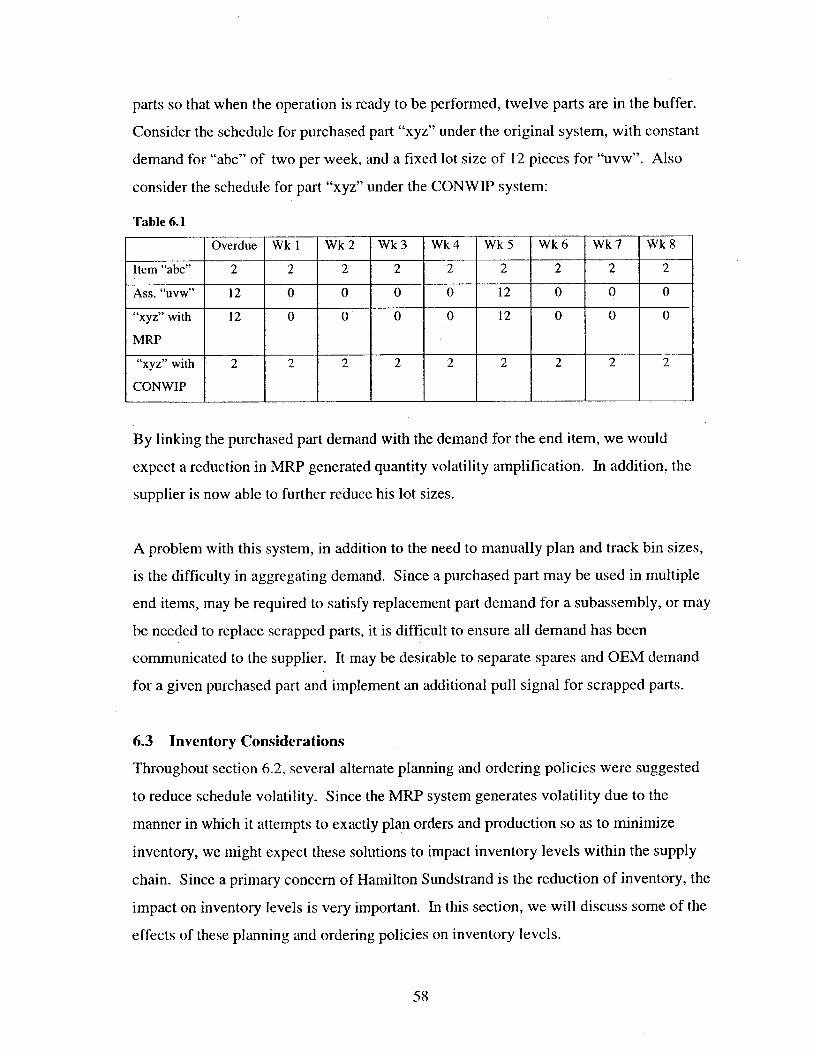
6.1. Supplier Communication................. .. .. ................ 496.2. Alternate Order Policies................... .................... ..................................... 526.3. Inventory Considerations ................. ......................................................... 586.4. Summary ...................................................... 64
7. Recomm endations and Conclusions .............................................................. 667.1. Reduce Lot Sizes, Use Fixed Lot Sizes and Work to Discrete Demand ........ 667.2 Pull System M anufacturing............................................................................. 687.3. Pull System with CONW IP or Hybrid Control................................................ 687.4. Future Research........................................................................................... 697 .5 . C on clu sion s ............................................................................................... . . 7 0
7
Page 8
8. Bibliography ................................................................................................... 71
9. Appendix: Schedule Volatility Analysis Method........................................... 72
8
Page 9
1. Introduction
The objective of this thesis is to discuss the sources of volatility in schedules created
using modem MRP systems. By analyzing actual schedule data obtained from Hamilton
Sundstrand, a division of United Technologies Corporation, it will be shown how the
MIRP system can produce highly volatile schedules. The resulting instability at the
purchased part level may be so high, in fact, that suppliers are unable to maintain
acceptable service levels without excessive inventory levels. Since suppliers may be
unwilling or unable to hold large amounts of inventory, with the corresponding inventory
costs and risk of obsolescence, downstream production may suffer when part shortages
occur.
This thesis will also demonstrate, using actual schedule data, how lot size policies in the
MRP system contribute to the problem by amplifying the magnitude of schedule changes.
These policies work in such a way that small changes to the master schedule may appear
as very large quantity changes to suppliers. The resulting amplification requires that
suppliers maintain much higher inventory levels for a given service level than would
otherwise be warranted based on the variation in aggregate customer demand.
Finally, some proposals for reducing schedule volatility are presented. The thesis also
examines some alternate planning and ordering methods being considered, and discusses
the probable ramifications on schedule volatility and inventory levels.
1.1 Background
The problem with schedule volatility in MRP systems is not new, nor is it a concern only
for Hamilton Sundstrand. In fact, one year earlier, a fellow Leaders for Manufacturing
internship was concerned with exactly this problem. Thomas Hoag (1999) at Pratt &
Whitney (another company within United Technologies) looked at various sources of
volatility in the MRP schedule and the cost of making changes to schedules. Based on
this analysis, he recommended rules regarding when a change should or should not be
made.
9
Page 10
Although we will use Hamilton Sundstrand's terminology for changes in purchasing or
production schedules, what we refer to as schedule volatility (or instability) is generally
described as nervousness in the academic literature. This term was used by Steele (1975)
to describe:
"...excessive changes to low-level requirements when there are no major
changes in the master schedule"
The problem with schedule volatility in MRP systems is in fact so widespread, that it is
discussed briefly in operations textbooks such as Arnold (1991) and Nahmias (1997).
Schedule volatility is caused by many factors, including changes in the master production
schedule (MPS), scrap and loss, changes in the bill of material, and changes in MIRP
system parameters. The factors leading to nervousness are discussed in more detail in
Steele (1975) and Mather (1977).
Although the causes of schedule volatility should be minimized so as to improve stability,
much of the problem with instability arises as a result of lot size policies. Steele (1975)
discusses how lot-sizing problems contribute to, and even amplify changes at low-levels
in the MIRP system. He also suggests the use of fixed order quantity lot sizes as opposed
to period of supply lot sizes to help stabilize MRP schedules. Mather (1977) expands on
this work and suggests that:
"...most reschedules that occur in MJRP programs today are not caused by
reactions to customer wishes. They result from application of
sophisticated mathematical routines for calculating lot-sizes. .."
He also presents some good examples demonstrating how lot-sizing issues contribute to
schedule volatility.
Although it has long been recognized that lot size problems contribute to schedule
volatility, it has been difficult to determine a good solution. Since lot sizes are
established to minimize total cost, recognizing that each purchase order or work order has
an associated fixed cost, some researchers have proposed assessing a cost to
10
Page 11
rescheduling. Kropp (1979) suggests incorporating the additional fixed cost of changing
the schedule into the logic used to dynamically determine the lot size in the MiRP system.
In theory, such a system would only make a change when, in fact, it is economically
justified. Kropp (1984) expands on this suggestion by proposing a modified Wagner-
Whitin algorithm that includes the "cost of nervousness" in the fixed costs.
Unfortunately, the difficulty in attaching a cost to instability or the complexity of
incorporating this logic into MRP systems may have prevented this solution from gaining
popularity.
Minifie (1986) suggests using dampening mechanisms to reduce the effect of changes on
low-level schedules. These mechanisms may include safety stock or safety lead-time,
time fences, and/or different lot sizing techniques. Time fences provide rules regarding
when changes can be made in the schedule. For example, a time fence may state that an
order cannot be deferred within four weeks of the scheduled production date.
These and other techniques to improve schedule stability were evaluated by Blackburn
(1986), using simulation to investigate the effectiveness of freezing the schedule within
the planning horizon, lot for lot policies after stage 1, safety stocks, forecast beyond the
planning horizon, and a change cost procedure. The fact that this simulation was
conducted using dynamic lot sizing algorithms such as Wagner-Whitin or Silver-Meal
makes it difficult to compare the results to Hamilton Sundstrand, who uses only very
simple lot size policies, such as fixed lot size or period of supply. However, it should be
noted that safety stock was helpful in reducing schedule volatility, however, since
relatively large levels of inventory were required, this method was judged ineffective on
the basis of cost.
Ho (1989) also used simulation to determine the affect of various lot sizing rules and
dampening procedures on cost and schedule volatility. This work concluded that a fixed
lot size rule significantly reduced the instability in the MRP schedules as compared to a
dynamic lot size rule such as lot-for-lot. However, the conclusion also suggested that the
reduction in schedule stability was balanced by an increase in total costs, since the fixed
II
Page 12
order quantity was more likely to result in a part shortage. The cost of this system with
additional safety stock was not evaluated.
Although considerable effort has been devoted to understanding schedule volatility and
using simulation to determine the theoretical benefits of various lotting policies and
dampening methods, there seems to be little or no data on the actual magnitude to which
lotting policies affect schedule volatility. Without such data, it may be difficult to
convince a company that a significant problem exists, or that simply addressing the
causes of instability may be insufficient to solve the problem. Although at least two
divisions of United Technologies have experienced significant problems with schedule
volatility, there was no clear understanding of the size of the problem, or the contribution
of lotting policies.
Almost all of the research to date has used simulation results to determine the
performance characteristics of various proposed solutions, without any data on the
functionality and actual benefits in real manufacturing environments. It is difficult to
convince companies to change procedures when the benefits cannot be quantified.
In addition, the implementation of complex algorithms to determine what size lots are
ordered or produced, or when to allow or forbid a schedule change may be hindered by
the inability of users to understand the logic. Although such systems may perform better,
users may like the ability to look at an MRP schedule and understand how it was
generated. This probably explains why Hamilton Sundstrand typically only uses fixed or
period-of-supply lot sizes, and why many MRP systems do not utilize more complex
algorithms.
This thesis uses actual schedule data to quantify the schedule volatility problem and the
effect of lotting policies. Based on this analysis, some relatively simple proposals are
suggested for reducing the amount of schedule instability experienced by suppliers.
These proposals are than evaluated based on results from former Sundstrand plants and
12
Page 13
using a simple analysis of inventory levels. It is believed that this will better convince
people of the nature of the problem and what steps can be taken to allow improvement.
1.2 Thesis Overview
Using actual schedule data collected over a fifteen-week period, this thesis presents
evidence that schedule volatility is a major contributor to poor on-time delivery from
suppliers. Suppliers are generally required to maintain approximately one to two months
worth of demand for each part in inventory, and discussions of schedule volatility and on-
time delivery often focus on why suppliers who maintain this inventory should be
expected to deliver even with schedule changes. This analysis demonstrates that
significantly higher levels of inventory are required to maintain acceptable service levels.
By comparing the volatility of two related schedules, it can be shown that lotting policies
contribute significantly to the problem of schedule instability. While the influence of
lotting policies on schedule instability has been discussed at length in the academic
literature, this analysis, using actual schedule data, demonstrates the magnitude to which
such policies contribute to the problem at Hamilton Sundstrand. This lends credibility to
the argument that schedule volatility can only be improved by addressing the lotting
policies used within the MRP system and the manner in which demand requirements are
communicated to suppliers.
1.3 Thesis Outline
This thesis is divided into seven sections: Introduction, Project Description, Problem
Definition, Schedule Volatility Analysis, Time Volatility Analysis, Proposals for
Reducing Volatility, and Conclusions / Recommendations. Section 1 (Introduction) gives
background to the problem of schedule volatility, how it may affect suppliers and
production, and prior research regarding volatility and lotting policies. Section 2
(Project Description) discusses the internship setting, and the main issues of concern for
the Purchasing Department of Hamilton Sundstrand. Section 3 (Problem Definition)
discusses some initial actions that were taken to deal with schedule volatility and
13
Page 14
describes some of the main sources of instability in the MiRP schedules. The next two
sections present the results of an analysis of approximately four months of schedule data
for purchased parts. Section 4 (Schedule Volatility Analysis) demonstrates the level of
instability that exists in these schedules, and the ramifications for suppliers' service level
and inventory. This section also demonstrates how lotting policies contribute to schedule
instability. While this section primarily focuses on quantity changes within the schedule,
Section 5 (Time Volatility Analysis) presents the results of an analysis of time volatility.
Section 6 (Proposals for Reducing Schedule Volatility) presents some suggestions for
reducing the impact of lotting policies on schedule instability and looks at the inventory
ramifications of these proposals. Finally, Section 7 (Conclusions / Recommendations)
suggests a course of action for improving schedule volatility over time.
14
Page 15
2. Project Description
This project was performed at the Hamilton Sundstrand Division of the United
Technologies Corporation. The focus of this project was an attempt to determine the root
cause(s) of excessive week to week changes in the quantity requirements of purchased
parts as seen in the schedules provided to suppliers. These changes are collectively
referred to as schedule volatility, and were perceived by Hamilton Sundstrand as
potentially the largest single cause of overdue shipments of parts from suppliers.
Overdue shipments were in turn considered a major cause of high Work-In-Process
(WIP) inventory levels and undesirable customer on-time service performance.
This section contains background material describing Hamilton Sundstrand, the
motivation for improving schedule volatility, an overview of the function of a typical
MRP system, and the suppliers' view of the schedule volatility problem.
2.1 Company Description
Hamilton Sundstrand is a large supplier of aerospace components for military and
commercial aircraft based in Windsor Locks, CT. It is a wholly owned subsidiary of the
United Technologies Corporation in Hartford, CT. Hamilton Sundstrand was formed
during the merger of Hamilton Standard and Sundstrand Corporation in 1999.
Hamilton Sundstrand supplies a large variety of aerospace components including jet
engine fuel controllers, jet engine starters, auxiliary power units (APUs) for aircraft, and
aircraft environmental control units (ECUs), as well as such products as propellers, space
suits and other space shuttle systems, and environmental systems for submarines. The
products can be generally categorized as high variety, high lead-time, relatively high cost
and low volume.
The business can be divided into two parts, Original Equipment Manufacturers (OEM)
and Aftermarket Replacement Parts (Spares). The OEM business is generally make-to-
order, with schedules being provided by customers as far as two years in advance. The
spares business is make-to-stock, with production schedules based on forecasts.
15
Page 16
The nature of the spares business makes forecasting difficult and often very inaccurate.
Hamilton Sundstrand provides spare parts for current production aircraft, as well as out-
of-production aircraft. Since the out-of-production-spares (OOPS) may be for planes
with very few aircraft still flying in the world, Hamilton Sundstrand is supporting parts
that may have gone into production 50 or 60 years ago. This makes forecasting and
obtaining purchased parts, particularly electronic components, very difficult. In such an
environment, Hamilton Sundstrand requires close working relationships with the supply
base to support changing needs and flexible production of low volume, obsolete parts.
2.2 Motivation
Starting at the beginning of 2000, the number of overdue shipments from suppliers began
to steadily rise. As the number of overdue shipments began to rise, production had
increasing difficulty completing finished items for delivery to customers. This resulted in
an increase in inventory levels, as WIP inventory grew. In addition, on-time delivery to
customers suffered, as Hamilton Sundstrand was unable to complete parts in the planned
lead-time. This in turn led to increased customer dissatisfaction.
Representatives from the purchasing department met with many of the suppliers with
particularly high levels of overdue parts. Specifically, they requested that the suppliers
identify areas of improvement and actions that would enable them to decrease their
overdue by 50%. The suppliers agreed to identify actions, but expressed their belief that
approximately 50% of the problem was caused by significant changes in the delivery
schedules provided weekly by Hamilton Sundstrand.
2.3 MRP System Overview
Hamilton Sundstrand uses a typical MIRP system to track customer requirements and
forecasted needs, plan production schedules, and determine purchase parts requirements.
The system used is J.D. Edwards, but is comparable with many of the popular MIRP
products including Oracle or SAP.
16
Page 17
The basic operation of the MRP system is to determine how many parts on what dates
must be delivered in order to meet customer demand. Similarly, the production start
dates of subassemblies manufactured in the factory are determined by the MRP system.
It does this by starting with the dates and quantity of expected customer demand (i.e.
when the end item is needed). This schedule may be either a firm order (as generally the
case with OEM parts) or a forecast schedule (as generally provided by the spares group).
Taking this Master Production Schedule (MPS), the system then determines what
components and what quantity of each component are used in the end product, based on a
Bill of Materials (BOM). Finally, the system determines the required delivery date of
purchased parts, and the required start date of production parts by subtracting the lead-
time for each component from the date of the demand. This is done for every end item
and for every level of assembly in an end item consisting of components built from other
assemblies that may in turn be composed of other sub-assemblies.
Consider the following examples:
End Item A is needed in 4 weeks and is built from assemblies Q and R
Assembly Q requires one week to build and is used once in Item A
Assembly R requires two weeks to build and is used twice in Item A
Thus, the MRP schedule would look like this:
Week I Week 2 Week 3 Week 4
Item A I
Assembly Q I
Assembly R 2
Assume Assembly R is composed of purchased parts x and y
Part x is used once in Assembly R
Part y is used three times in Assembly R
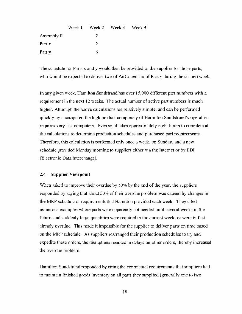
Thus, the MRP schedule for the purchased parts would look like this:
17
Page 18
Week 1 Week 2 Week 3 Week 4
Assembly R 2
Part x 2
Party 6
The schedule for Parts x and y would then be provided to the supplier for those parts,
who would be expected to deliver two of Part x and six of Part y during the second week.
In any given week, Hamilton Sundstrand has over 15,000 different part numbers with a
requirement in the next 12 weeks. The actual number of active part numbers is much
higher. Although the above calculations are relatively simple, and can be performed
quickly by a coinputer, the high product complexity of Hamilton Sundstrand's operation
requires very fast computers. Even so, it takes approximately eight hours to complete all
the calculations to determine production schedules and purchased part requirements.
Therefore, this calculation is performed only once a week, on Sunday, and a new
schedule provided Monday morning to suppliers either via the Internet or by EDI
(Electronic Data Interchange).
2.4 Supplier Viewpoint
When asked to improve their overdue by 50% by the end of the year, the suppliers
responded by saying that about 50% of their overdue problem was caused by changes in
the MRP schedule of requirements that Hamilton provided each week. They cited
numerous examples where parts were apparently not needed until several weeks in the
future, and suddenly large quantities were required in the current week, or were in fact
already overdue. This made it impossible for the supplier to deliver parts on time based
on the MRP schedule. As suppliers rearranged their production schedules to try and
expedite these orders, the disruptions resulted in delays on other orders, thereby increased
the overdue problem.
Hamilton Sundstrand responded by citing the contractual requirements that suppliers had
to maintain finished goods inventory on all parts they supplied (generally one to two
18
Page 19
months of average demand). The feeling was that if the supplier was in fact fulfilling this
requirement, there should be no problem with adjusting to schedule changes.
The suppliers maintained they were indeed fulfilling the contract, but that a schedule
change was often so large in magnitude, that it would deplete the entire inventory on the
part, and still the supplier would be overdue on the remaining quantity. Later audits
suggested that the suppliers were generally maintaining inventory as required.
2.5 Summary
In summary, Hamilton Sundstrand manufacturers a large variety of components in low
quantities and purchases many thousands of different components from the supply base.
Throughout the year 2000, the number of overdue shipments from suppliers increased
steadily, leading to large WIP inventories and unsatisfactory customer service levels.
After meeting with suppliers, Hamilton Sundstrand determined that weekly changes in
the delivery schedules provided to suppliers were both frequent and often very large in
magnitude. These changes certainly contributed to supplier overdue, and may in fact
have been a very large factor (as high as 50%) in the level of overdue shipments.
19
Page 20
3. Problem Definition
In order to lower Direct Material Purchase (DMP) cost and reduce on-hand inventory,
Hamilton Sundstrand has signed Long-Term Agreements (LTAs) with many suppliers.
Suppliers on LTA are provided a schedule of requirements each week either over the
Internet or by EDI. This schedule contains weekly quantity requirements for the next
eight weeks, and monthly quantity requirements for the following ten months, with any
remaining quantity lumped together in the 1 3th month. The suppliers use these schedules
for long-term capacity planning, raw material planning, shop schedule planning, and
shipment data. Unfortunately, many of the parts on this schedule are seemingly subject
to large changes, in both quantity and date. These changes are such that the supplier,
even with one to two months of inventory on the shelves, is often unable to support the
schedule requirements.
Not only do the magnitude of the changes create problems with the supplier shipping on-
time, but the frequent changes require considerable time and effort, both to track, and to
reload the shop accordingly. This reduces the actual capacity of the supplier's operation
and can thereby further increase the number of late shipments.
Based on suppliers' statements and Hamilton Sundstrand's initial investigation, this
problem could account for as much as 50% of all overdue parts from a supplier.
Interestingly enough, suppliers maintain that generally speaking, given a long enough
period of time (for example a year), the quantity shipped in that year matches the original
forecast. By reducing schedule volatility, Hamilton Sundstrand should be able to
improve supplier on-time performance and potentially reduce inventory levels at the
supplier.
3.1 Problem Scope
The schedule volatility problem includes all parts that are supplied by an external
supplier for both OEM and spares needs. In fact, the MRP system lumps all requirements
for common parts within a defined operating unit together. For this project, we have
limited our investigation to legacy Hamilton locations in Connecticut. This excludes
20
Page 21
international operations, Hamilton operations outside of Connecticut, and all legacy
Sundstrand operations. Within this definition, there are three production branch plants
and two spares branches.
By lumping all requirements within these three branch plants and two spares branches,
the MRP system avoids the possibility that a supplier may have to ship many small
shipments of the same part to different location. All the requirements for a part are sent
to one branch plant (the primary branch), and requirements for other branch plants are
handled through interplant transfers. In this case, the primary branch acts like a supplier
to all the other branches.
During the initial investigation, we considered only changes that resulted in an overdue
part, where the part was not previously overdue, and where, during the previous week,
the supplier's schedule did not show a requirement in the current week. We call such a
case a "surprise overdue" part. This means that the supplier had no reason to believe the
part would be overdue when the new schedule was created during the weekend; hence,
the part was a surprise overdue.
3.2 Initial Actions
Initially, we limited our investigation to surprise overdue parts. These parts were
particularly important because suppliers were being penalized for failing to deliver parts
that they had no reason to believe were needed. As such, these parts were a major source
of concern to both Hamilton Sundstrand and suppliers. By examining the source of the
schedule change that caused these parts to be suddenly overdue, we hoped to better
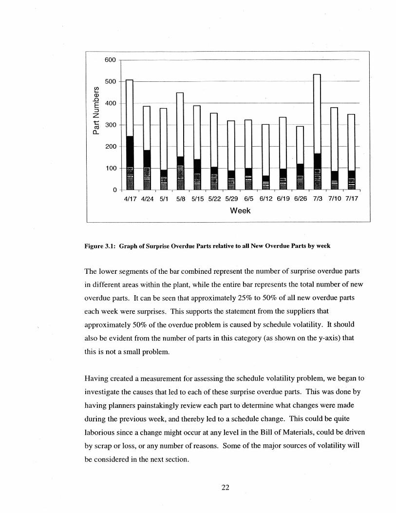
understand the sources of schedule volatility. Figure 3.1 shows a graph of surprise
overdue by production area as a part of all the new parts that were overdue that week.
(New overdue parts are parts that were not overdue the previous week. A surprise
overdue can also occur for a previously overdue part, if the supplier delivered the
overdue requirement and believed they were thereby caught up. However, for
simplicity's sake, we ignore such occurrences).
21
Page 22
600
500C,,
E 400-
300
200-
100-
4/17 4/24 5/1 5/8 5/15 5/22 5/29 6/5 6/12 6/19 6/26 7/3 7/10 7/17
Week
Figure 3.1: Graph of Surprise Overdue Parts relative to all New Overdue Parts by week
The lower segments of the bar combined represent the number of surprise overdue parts
in different areas within the plant, while the entire bar represents the total number of new
overdue parts. It can be seen that approximately 25% to 50% of all new overdue parts
each week were surprises. This supports the statement from the suppliers that
approximately 50% of the overdue problem is caused by schedule volatility. It should
also be evident from the number of parts in this category (as shown on the y-axis) that
this is not a small problem.
Having created a measurement for assessing the schedule volatility problem, we began to
investigate the causes that led to each of these surprise overdue parts. This was done by
having planners painstakingly review each part to determine what changes were made
during the previous week, and thereby led to a schedule change. This could be quite
laborious since a change might occur at any level in the Bill of Materials, could be driven
by scrap or loss, or any number of reasons. Some of the major sources of volatility will
be considered in the next section.
22
Page 23
3.3 Sources of Volatility
In a large company, producing a wide variety of end items, with a large number of
customers, and a large number of purchased parts, literally hundreds of people are
capable of making changes which effect the schedule of purchased parts. The popular
description of the field of "Chaos", in which a butterfly flapping its wings can affect the
weather hundreds of miles away, is an apt depiction of the situation that occurs in this
environment. We will consider five areas in which schedule changes can be generated.
These five areas are: Demand Changes, Inventory Changes, Work Order Changes, MRP
Setting Changes, and Message Processing. This listing is not meant to provide an
exhaustive description of all possible sources of volatility, but should give the reader a
good idea of many possible scenarios that arise.
3.3.1 Demand Changes
Customer demand changes are the most obvious cause of schedule changes. This
includes both OEM demand, generally for an end item, as well as spares demand, which
may be for an end item, for a subassembly, or for a purchased part.
OEM customers generally provide a schedule for many months, or even years into the
future. Since many aerospace customers are working with several years of backlog
orders and military customers generally have fixed schedules from the armed forces,
these schedules tend to be very reliable. If demand changes occur, they are generally
very small in magnitude or relatively far into the future:
Spare parts are built to a forecast. For reasons that are out of the scope of this thesis,
forecasts in the aerospace industry tend to be very inaccurate. As such, the production
schedules generated as a result of these forecasts are subject to larger magnitude, more
frequent changes as compared to OEM schedules. In addition, Aircraft On-the Ground
orders (AOGs) mean that a very expensive aircraft is not flying due to a need for a
replacement part. These orders typically are given very high priority.
23
Page 24
In order to dampen the impact of forecast inaccuracies on supplier schedules, the spares
group works to very strict rules governing when they are permitted to change a
production schedule. Generally speaking, they cannot place an order for a part or move a
requirement to an earlier date, if this change occurs within the longest lead-time of any
component in the assembly. Furthermore, they cannot move a requirement to a later date
if the current requirement date is within three months of the day on which they wish to
make the change. Exceptions to the above rules can be made at the discretion of planners
or managers, if the movement will not affect inventory coverage through the longest lead-
time of any component part, or if the change is necessary to support an AOG. If indeed
these rules are being followed, spares should not be a big contributor to schedule
volatility.
3.3.2 Inventory Changes
The MRP system determines the supplier schedule by looking at the date of all
requirements and the current available inventory. In other words, if there are already ten
parts in stock, the first supplier requirement will be driven by the date when the II' part
is needed. Therefore, schedule changes can occur not only as a result of date changes, but
also as a result of changes in inventory levels. In a perfect world, inventory would
change only when a part was built, but in practice inventory changes can occur for other
reasons. The following is a partial list of factors that cause inventory to change:
> Scrap or Loss (can be negative if parts are found or reworked...)
> Parts are expensed (removed from inventory) before being used
> Parts transferred to another branch plant
> Misallocation of parts (generally considered a work order change)
It is a reality of manufacturing that mistakes will occur, that processes will go out of
control, and therefore that unusable parts will be created. Although most MRP systems
allow a scrap factor to be used so that additional requirements will be purchased to
account for scrap, the low volume nature of the aerospace industry is not conducive to the
use of a scrap factor. Generally speaking, Hamilton Sundstrand does not use a scrap
factor for any parts. Also, Hamilton Sundstrand uses a large number of very small,
24
Page 25
inexpensive parts and often some of these parts are lost. Typically, Hamilton Sundstrand
has better than a 95% inventory accuracy (meaning that the quantity in inventory as
determined by a physical inventory count agrees with the quantity shown in MRP), so we
would not expect this to be a major source of volatility.
Another cause of inventory inaccuracy occurs frequently at Hamilton Sundstrand. There
is a classification of parts, called binstock parts, which are generally very inexpensive,
commodity components like standard washers or fasteners. Rather than force the
operators to go to the storeroom every time they need a single washer, the operators take
a relatively large quantity and fill a small drawer at their workstation. To prevent the
need to count every cheap little part at every workstation whenever inventory is counted,
these parts are expensed immediately upon removal from the storeroom. When the parts
are expensed, they no longer appear in inventory, even though there are outstanding
requirements in the MRP system for those parts, and those parts physically exist in the
factory. In other words, the operator may need two washers to build an assembly, so he
goes to the storeroom and removes 50 washers. In doing so, he may remove the entire
supply of that washer at the storeroom. These 50 washers immediately disappear from
inventory in the MRP system, which now thinks there are no parts in the building, even
though 48 pieces still exist on the operator's desk. The operator may use the 48 pieces
over a period of several weeks, to build orders as scheduled by the MRP system.
However, the entire time, the MIRP system thinks it needs to order 48 washers so as to
complete the outstanding orders. The system will therefore issue an order for 48 pieces.
In the meantime, while the supplier is trying to ship 48 pieces he did not previously
believe were needed, the operator may in fact finish building the items that use those
washers. In doing so, the MRP system no longer sees a need for the washers, and may
cancel the order.
There are many binstock parts used at Hamilton Sundstrand and the contribution of these
parts to schedule volatility is widely understood. However, the inexpensive, commodity
nature of binstock parts has generally meant that they were ignored. It was often felt that
due to their commodity nature, suppliers should be able to react quickly to schedule
25
Page 26
changes. It should be noted that binstock parts are excluded from the calculation of
surprise overdue (as well as from the on-time delivery metrics). This means that the
extent of the schedule volatility is really only seen by suppliers, who treat binstock parts
no differently than normal parts, and therefore see more schedule movement than
Hamilton Sundstrand actually tracks in their metrics.
Part transfers generally should occur as the result of a legitimate requirement from
another branch plant. As such, transfers generally should not cause unforeseen changes
in inventory levels. A problem did exist in the implementation of the MRP system at
Hamilton Sundstrand that could lead to a circular demand for transferred parts. In such a
case, the transfer of parts from plant A to plant B, would generate a need to transfer the
same part back from plant B to plant A. This problem did not appear to be a factor in the
generation of schedule volatility and will not be considered in this thesis.
Part misallocation generally means that inventory was used to satisfy a later requirement,
thereby leaving the inventory levels insufficient to satisfy an earlier requirement. The
supplier would normally expect that inventory would be applied to the earliest
requirement, then to the next earliest requirement, and so forth chronologically. Consider
the following example: Area A has a requirement for 5 pieces of part x this week, Area
B has a requirement for 5 pieces of part x also, but the requirement is not schedule until
three weeks from now. For some reason, Area B consumes their requirement of part x,
leaving zero parts in inventory for Area A. Next week, the supplier for part x will see an
overdue requirement for 5 pieces. Since generally part misallocation occurs as a result of
changes in work orders (i.e. Area B built their work order three weeks early), this
problem is usually included in work order changes.
3.3.3 Work Order Changes
The MRP system works by determining when assemblies and end items need to be built,
and when purchased parts need to arrive, to support a given demand. Instructions to the
shop regarding when items should be built are called work orders. When a person from
the shop accepts the recommendation from the MRP system, the work order is given a
26
Page 27
number and is called afirm work order. Any time that this person firms up a work order
for a different date or quantity as suggested by the MRP system, or anytime that a person
changes a firm work order, this change may result in a schedule change for a supplier.
These changes may occur as a result of incorrectly following procedures, or may be a
legitimate change. The following work order changes occur most frequently:
> Splitting/Combining Work Orders
> Moving Work Orders
> Allocating Parts to Work Orders out of Sequence
The quantity on the work order is determined using various rules. These rules dictate the
lot size used for a work order and are set by planners with input from the shop floor. If
the factory changes work order quantities for a given part on a regular basis, this would
suggest that a different rule should be used. Unfortunately, no rule can anticipate the
daily changing needs of the shop floor. Changing the quantity on a work order generally
occurs when an area in the plant wishes to run several work orders together to save setup
time. Work orders may also be combined for many other reasons. For example, a piece
of equipment used in the manufacturing process may need to undergo a lengthy
refurbishment and parts are being completed ahead of schedule in anticipation of the
machine being unavailable. Similarly, a large work order may be split into several work
orders. Such a change may occur if there is insufficient inventory for every component
part to complete the entire work order quantity.
Work orders may be moved for a variety of reasons. The changing needs and conditions
that arise during the daily operations of the plant may dictate a production schedule that
differs from the original MRP planning. The larger the plant and the larger the number of
products, the more likely these changes will occur. For example, if an important
purchased part cannot be delivered on time, the factory may elect to move the work order
that uses this part to a later date, and elect to build other parts instead. When the work
orders are manually changed to reflect this, the resultant supplier schedules will reflect
the movements.
27
Page 28
The largest single cause of schedule volatility due to work order changes is misallocation.
By this we generally mean that parts were allocated to work orders out of sequence. This
can occur when a part is used in different areas. If one area builds parts further in
advance than another area, inventory may be applied to work orders in a manner that
differs from the sequence that the MIRP system had planned.
3.3.4 MRP Setting Changes
There are many factors that are input into the MRP system that control how the system
determines the dates and quantities for work orders and purchase parts. Changes to these
factors can result in changes in the supplier schedules. The main factors that affect the
MIRP planning process are:
> BOM relationships and quantities
> Manufacturing Lead Times
> Safety Stock Level
> Receiving Lead Time
> Lot Size Policies
All of the requirements planning are based on end item demand and a corresponding
BOM for this end item. If a change is made in the BOM, a schedule change may result,
even without a change in end item demand. For example, if the BOM specifies the end
item uses part x and then is changed to use part x', the schedule for part x will reflect this
change. If the BOM specifies that an end item uses two feet of material y, and then is
changed to require 2.2 feet of material y, the corresponding requirement for material y
will change.
The MRP system also uses a fixed manufacturing lead time to determine when the shop
should start building a work order so as to meet a given customer demand. If the system
is set for a lead-time of two weeks, and subsequent analysis determines that the process
actually requires three weeks, the lead-time in the system should be changed to reflect
this. This change will, however, require that suppliers deliver the component parts one
week earlier.
28
Page 29
Generally, the MiRP system does not plan for material to arrive until the inventory level
reaches zero. In many situations, it may be practical to have the MRP system maintain
some minimum level of inventory. By setting a safety stock level, the MiRP system will
attempt to order material so that the inventory never falls below this level. Changes to
the level will be reflected in changes to the supplier schedules.
Receiving lead-time is the time it takes for material that arrives on the dock to be
processed and moved to the stockroom or manufacturing floor. If the MRP system
determines that parts are required for a work order on Thursday, and the receiving lead-
time is two days, the supplier schedule will show a need for parts on Tuesday. Typically
this lead-time is relatively small, however, in some cases it may be considerably longer
so as to be used as a safety factor to insure that problem suppliers deliver the parts before
they are actually needed.
The final factor that affects MIRP planning is the lotting policy. There are two main
lotting policies used at Hamilton Sundstrand. These are: fixed order quantity and period
of supply. Fixed order quantity means that the MRP system always orders parts from
suppliers or plans work orders in a given quantity. Period of supply means that the MIRP
system looks out in the future for a given period of time, lumping all of the requirements
for the part during that period into one order. Changes in lotting policy can cause
changes in the supplier schedule. In addition, lotting policies themselves can have a
dramatic impact on schedule volatility and will be discussed in great detail later in the
text.
3.3.5 Message Processing
The MRP system used by Hamilton Sundstrand is driven by messages. This means that
the system generates messages instructing different users what tasks should be performed
and when they should be performed. A typical message to the shop floor might be to
build five of part x on a specific date. A typical message to a buyer might be to purchase
five of component y on a specific date. For the system to work correctly, every person
29
Page 30
who works with the system must answer their messages without making any changes.
Failure to answer a message, or performing a task differently than suggested in the
message, may cause changes that appear as schedule volatility to the suppliers.
An example of an incorrect response to a message was given in the work order changes
section. The system suggests a quantity and date for a work order (a message) and the
shop floor person chose to build a different quantity on a different date when he or she
created the firm work order.
Other messages might suggest that a purchase order or work order should be completed
earlier (expedited) or later (deferred) or cancelled. Purchase orders or work orders might
receive a message to be split into two or more purchase orders or work orders. In many
cases, acting on a message may cause a schedule change (for example as a result of a
customer demand change), while failing to act on a message may also cause a schedule
change (if the shop floor reschedules a work order, the MRP system might automatically
reschedule the corresponding purchase orders).
3.3.6 Pareto Results
This lengthy description of sources of volatility in the MRP system should provide some
idea of the difficulty in determining the main factors driving supplier schedule volatility.
In order to better understand what the leading causes were, Hamilton Sundstrand planners
spent hours each week determining the root cause behind every part on the surprise
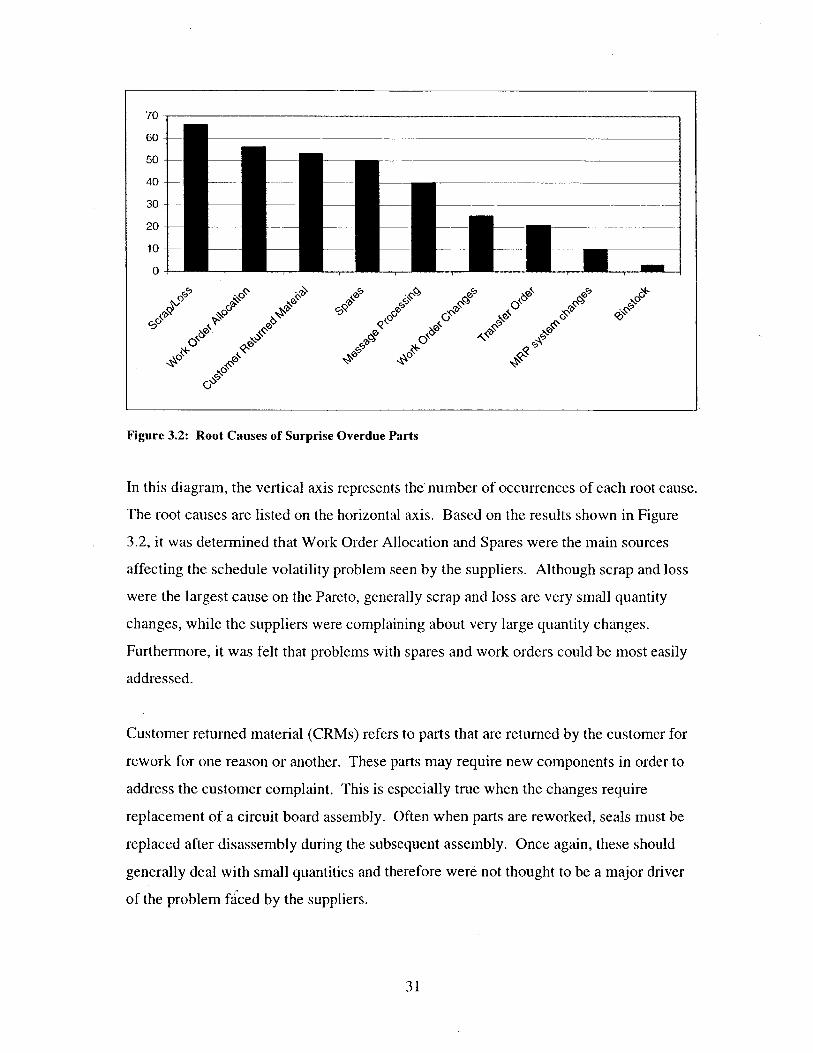
overdue list. The results are shown in a Pareto diagram in Figure 3.2.
30
Page 31
70
60--
50
40 -
30 ______
20-
0
4''
Figure 3.2: Root Causes of Surprise Overdue Parts
In this diagram, the vertical axis represents the number of occurrences of each root cause.
The root causes are listed on the horizontal axis. Based on the results shown in Figure
3.2, it was determined that Work Order Allocation and Spares were the main sources
affecting the schedule volatility problem seen by the suppliers. Although scrap and loss
were the largest cause on the Pareto, generally scrap and loss are very small quantity
changes, while the suppliers were complaining about very large quantity changes.
Furthermore, it was felt that problems with spares and work orders could be most easily
addressed.
Customer returned material (CRMs) refers to parts that are returned by the customer for
rework for one reason or another. These parts may require new components in order to
address the customer complaint. This is especially true when the changes require
replacement of a circuit board assembly. Often when parts are reworked, seals must be
replaced after disassembly during the subsequent assembly. Once again, these should
generally deal with small quantities and therefore were not thought to be a major driver
of the problem ficed by the suppliers.
31
Page 32
3.4 Initial Results
Based on the results of the Pareto analysis, Hamilton Sundstrand implemented several
corrective actions. These included:
> Reduction of the number of people who could handle work orders
> Re-Training on work order handling
> Detailed tracking and analysis of work order changes
> Detailed tracking and analysis of spares sales order changes
After implementing the changes and tracking work order and spares changes for many
weeks, no noticeable improvement was seen. Improvement was measured by reduction
in surprise overdue (Figure 3.3 shows the surprise overdue results for the remainder of
2000) and by subjective analysis from the supply base. Although improvement was
limited, the tracking did uncover the following facts:
> Many work orders and spares sales orders were changed manually each week
> These changes were generally done correctly, and for correct reasons
> The changes were generally small in magnitude compared to the changes noted by
the suppliers
> The MRP system automatically made many more changes each weekend when it
was run than were manually made during the week
600
500
400- -
300-
200-
100 --
Figure 3.3: Surprise overdue (unshaded) compared to total new overdue (entire bar)
32
Page 33
3.5 Summary
The MRP system is a very complex system, with many manual interactions, and many
opportunities for changes that create schedule volatility. Generally people make changes
for the right reasons, using the correct methods, and therefore, attempting to reduce
schedule volatility through training and tracking are ineffective. Finally, the magnitude
of changes made manually, appear small relative to the magnitude of changes about
which the suppliers complained, and the number of changes made manually appear small
relative to the number of changes made by the system.
Based on this summary, we determined that the schedule volatility must result from some
mechanism within the MRP system. It seemed clear that the system must be in some way
magnifying or amplifying the changes input into the system, thereby creating a much
larger change at the output of the system - the supplier schedules. Furthermore, we felt
that the only mechanism capable of this amplification were the lot size policies used
throughout the MRP system. As discussed in the Introduction, lotting policies can lead to
MRP nervousness. In order to understand the magnitude of this effect, we collected and
analyzed schedule data.
33
Page 34
4. Schedule Volatility Analysis
In order to determine the effect of lotting policies on schedule volatility, we measured the
number of schedule changes and the average magnitude of the changes for a large sample
of parts (over 2000 randomly selected part numbers). We compared the volatility of
these parts using two different schedules produced by the MRP system. The first
schedule we will term the "Supplier Schedule" and it refers to the schedule of
requirements that is provided to the suppliers for their production planning and shipping
use. The second schedule is what we term "Discrete Demand" and this refers to the
internal schedule used by buyers and expeditors. The main difference between the two
schedules is the application of a lotting policy based on a predefined part Strata Code.
This section will demonstrate how lotting policies might affect schedule volatility, define
how Strata Codes are used at Hamilton Sundstrand, and present evidence that lotting
policies actually amplify the magnitude of small schedule changes in a manner which is
very disruptive to suppliers. For detailed information regarding the schedule volatility
analysis, refer to the Appendix.
4.1 Lotting Policies
Companies frequently apply lotting policies to take advantage of economies from running
larger batches of product or purchasing in bulk. Setup times and costs may dictate that
large quantities (as compared to demand) be produced at one time. Frequently suppliers
offer discounts to customers purchasing large quantities. Even with the extensive use of
long-term agreements at Hamilton Sundstrand, in which suppliers agree to supply parts
for a fixed price, there are often minimum order sizes. In addition, transportation
economies dictate that small, inexpensive parts be shipped at less frequent intervals.
For these reasons, MRP systems provide functionality to automatically lot production of
parts or purchasing of parts. Generally, there are two types of lotting policies used at
Hamilton Sundstrand: fixed lot sizes, and period of supply. While both lotting policies
are used, we will primarily focus on period of supply policies and their relation to the
supplier schedule. Examples of both policies are presented in the next sections.
34
Page 35
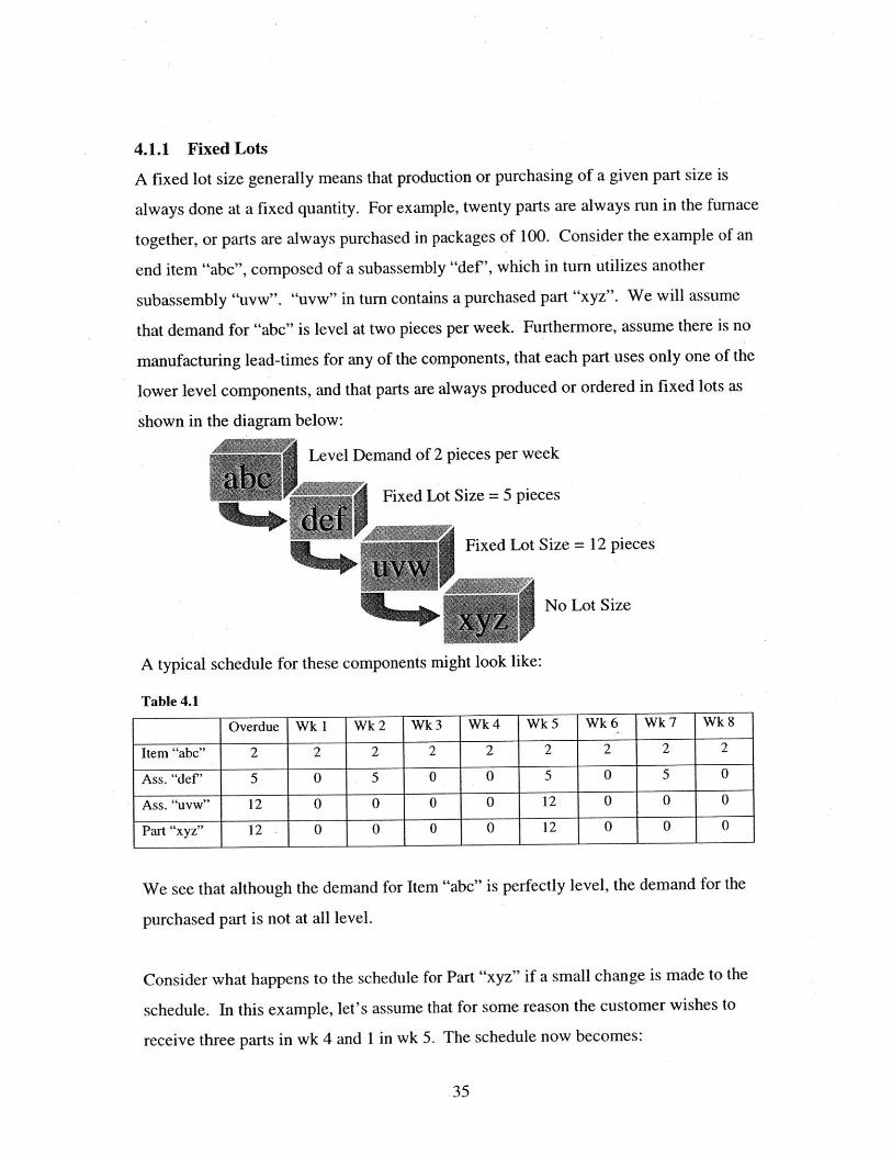
4.1.1 Fixed Lots
A fixed lot size generally means that production or purchasing of a given part size is
always done at a fixed quantity. For example, twenty parts are always run in the furnace
together, or parts are always purchased in packages of 100. Consider the example of an
end item "abc", composed of a subassembly "def", which in turn utilizes another
subassembly "uvw". "uvw" in turn contains a purchased part "xyz". We will assume
that demand for "abc" is level at two pieces per week. Furthermore, assume there is no
manufacturing lead-times for any of the components, that each part uses only one of the
lower level components, and that parts are always produced or ordered in fixed lots as
shown in the diagram below:
Level Demand of 2 pieces per week
3 Fixed Lot Size = 5 pieces
Fixed Lot Size = 12 pieces
No Lot Size
A typical schedule for these components might look like:
Table 4.1
Overdue Wk I Wk 2 Wk 3 Wk 4 Wk 5 Wk 6 Wk 7 Wk 8
Item "abc" 2 2 2 2 2 2 2 2 2
Ass. "def' 5 0 5 0 0 5 0 5 0
Ass. "uvw" 12 0 0 0 0 12 0 0 0
Part "xyz" 12 0 0 0 0 12 0 0 0
We see that although the demand for Item "abc" is perfectly level, the
purchased part is not at all level.
demand for the
Consider what happens to the schedule for Part "xyz" if a small change is made to the
schedule. In this example, let's assume that for some reason the customer wishes to
receive three parts in wk 4 and 1 in wk 5. The schedule now becomes:
35
Page 36
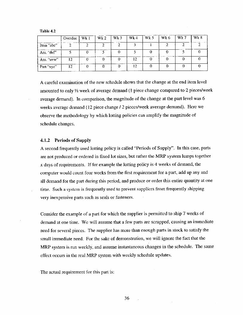
Table 4.2
Overdue Wk I Wk 2 Wk 3 Wk 4 Wk 5 Wk 6 Wk 7 Wk 8
Item "abc" 2 2 2 2 3 1 2 2 2
Ass. "def' 5 0 5 0 5 0 0 5 0
Ass. "uvw" 12 0 0 0 12 0 0 0 0
Part "xyz" 12 0 0 0 12 0 0 0 0
A careful examination of the new schedule shows that the change at the end item level
amounted to only /2 week of average demand (1 piece change compared to 2 pieces/week
average demand). In comparison, the magnitude of the change at the part level was 6
weeks average demand (12 piece change / 2 pieces/week average demand). Here we
observe the methodology by which lotting policies can amplify the magnitude of
schedule changes.
4.1.2 Periods of Supply
A second frequently used lotting policy is called "Periods of Supply". In this case, parts
are not produced or ordered in fixed lot sizes, but rather the MRP system lumps together
x days of requirements. If for example the lotting policy is 4 weeks of demand, the
computer would count four weeks from the first requirement for a part, add up any and
all demand for the part during this period, and produce or order this entire quantity at one
time. Such a system is frequently used to prevent suppliers from frequently shipping
very inexpensive parts such as seals or fasteners.
Consider the example of a part for which the supplier is permitted to ship 7 weeks of
demand at one time. We will assume that a few parts are scrapped, causing an immediate
need for several pieces. The supplier has more than enough parts in stock to satisfy the
small immediate need. For the sake of demonstration, we will ignore the fact that the
MRP system is run weekly, and assume instantaneous changes in the schedule. The same
effect occurs in the real MRP system with weekly schedule updates.
The actual requirement for this part is:
36
Page 37
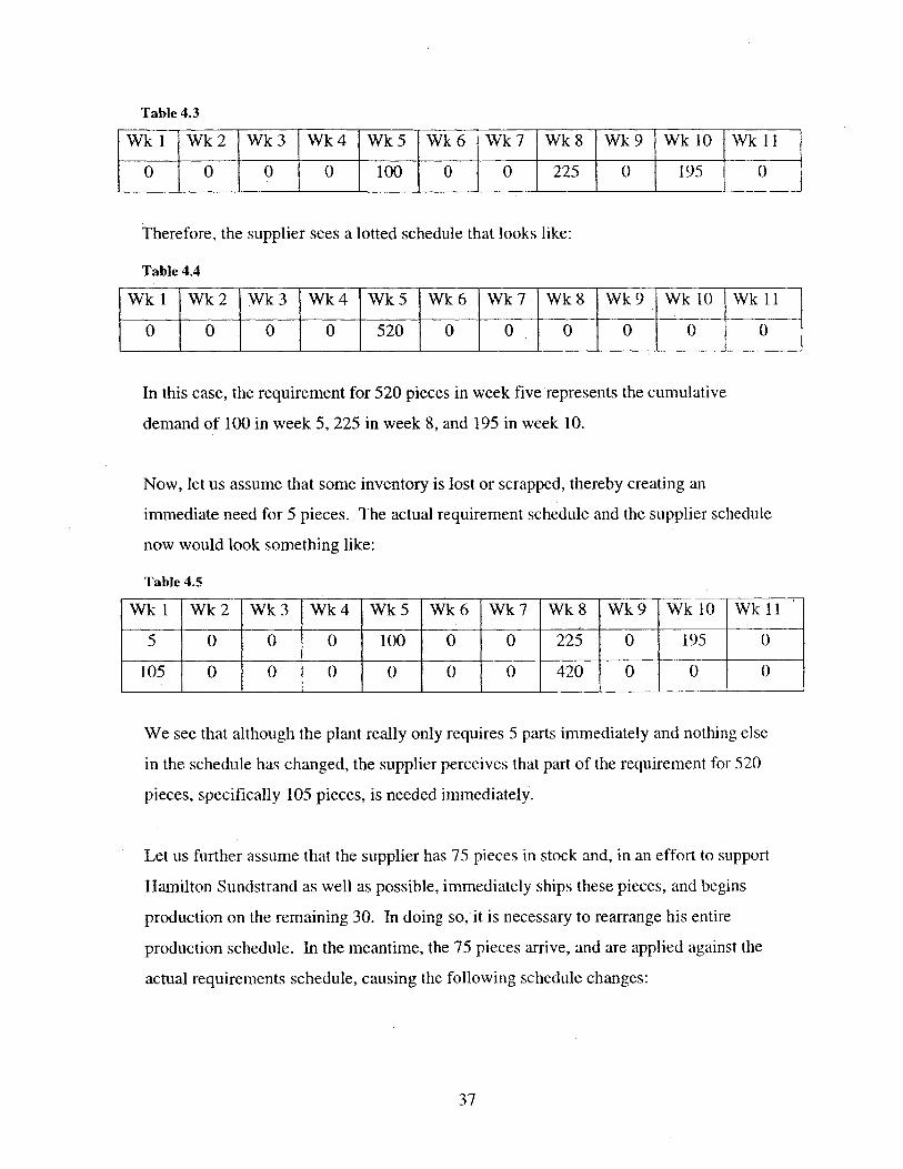
Table 4.3
Wkl Wk2 Wk3 Wk4 Wk5 Wk6 Wk7 Wk8 Wk9 WkIO Wkll
0 0 0 0 100 0 0 225 0 195 0
Therefore, the supplier sees a lotted schedule that looks like:
Table 4.4
Wkl Wk2 Wk3 Wk4 Wk5 Wk6 Wk7 Wk8 Wk9 WklO Wkll
0 0 0 0 520 0 0 0 0 0 0
In this case, the requirement for 520 pieces in week five represents the
demand of 100 in week 5, 225 in week 8, and 195 in week 10.
cumulative
Now, let us assume that some inventory is lost or scrapped, thereby creating an
immediate need for 5 pieces. The actual requirement schedule and the supplier schedule
now would look something like:
Table 4.5
Wkl Wk2 Wk.3 Wk.4 Wk.5 Wk6 Wk7 Wk.8 Wk9 WklO Wkll
5 0 0 0 100 0 0 225 0 195 0
105 0 0 0 0 0 0 420 0 0 0
We see that although the plant really only requires 5 parts immediately and nothing else
in the schedule has changed, the supplier perceives that part of the requirement for 520
pieces, specifically 105 pieces, is needed immediately.
Let us further assume that the supplier has 75 pieces in stock and, in an effort to support
Hamilton Sundstrand as well as possible, immediately ships these pieces, and begins
production on the remaining 30. In doing so, it is necessary to rearrange his entire
production schedule. In the meantime, the 75 pieces arrive, and are applied against the
actual requirements schedule, causing the following schedule changes:
37
Page 38
Table 4.6
Wkl Wk2 Wk3 Wk4 Wk5 Wk6 Wk7 Wk8 Wk9 WkO Wkl11
0 0 0 0 30 0 0 225 0 195 0
0 0 0 0 450 0 0 0 0 0 0
The 75 pieces satisfy the demand for 5 in week 1, as well as part of the demand for 100 in
week 5. Meanwhile, the supplier schedule now shows the first need in wk 5. The
supplier is forced to hold on to the 30 pieces he just made, after having disrupted his
production schedule to produce these parts against a perceived immediate need.
Furthermore, he needs to plan production of the remaining 420 pieces three weeks earlier.
Here again we see how small changes in the schedule can be converted to very large
changes in the supplier schedule due to lotting policies.
It is important to note that lotting policies have a second effect. If the requirement for
195 pieces in wk 10 as shown in Table 4.6 were suddenly needed one week earlier, the
supplier would see absolutely no change. In other words, if changes occur entirely within
the lotting period, suppliers will see no affect. In this situation, lotting policies actually
serve to dampen the effect of schedule volatility.
We therefore see two competing affects of lotting policies: in general, we would expect
lotting policies will reduce the number of changes in the supplier schedule, while
simultaneously increasing the magnitude of changes that do occur. It is therefore
important to determine the relative occurrences of these affects so as to understand which
affect is dominant.
4.1.3 Strata Policy
Hamilton Sundstrand provided a unique opportunity to determine the impact of lotting
policies on schedule volatility. There are two frequently used schedules for purchased
parts that are produced by the MRP system each week. These two schedules differ
primarily in the application of a period of supply lotting policy. The schedule for actual
38
Page 39
part requirements is the Discrete Demand schedule, and is used by the purchasing
department to manually order parts from suppliers that are not on long-term agreement.
The bulk of suppliers, however, receive a Supplier Schedule, in which requirements are
lotted based on a Strata Code.
All parts are given a Strata Codes of A, B, C or D. The correct code is determined for
each part based on the prior year's annual dollar volume. Strata A represents the parts
with the highest annual dollar volume, and are therefore generally the most expensive
parts. Strata D parts are the lowest dollar volume, and are generally the least expensive
parts.
Both Strata A and B parts are lotted in weekly periods, that means that suppliers only
ship one week of demand, while Strata C parts are lotted in 8 week periods, and Strata D
parts are lotted in 17 week periods. With perfectly stable schedules, this means that
suppliers would ship Strata A and B parts at most weekly, Strata C parts every two
months, and Strata D parts every four months.
4.2 Supplier Schedule Volatility
Using the analysis method described in the Appendix, we examined the schedules of
2020 parts selected at random. We measured the number of schedule changes and the
average magnitude of the schedule changes that the supplier would have seen looking at
an eight-week schedule. For this thesis we define the schedule for a part by lumping all
requirements for that part during an entire week (from Monday through Sunday) together.
We consider a time horizon consisting of eight of these weekly "buckets" for consecutive
weeks, hence, the eight-week schedule. In this definition, a schedule change means that
when the new schedule was created on the following Sunday MRP run, one or more of
the eight weekly lumped quantity requirements has changed.
For the analysis, we looked at fifteen consecutive MRP schedules. We compared the first
schedule (created in this case in the beginning of October) with a schedule created one
week later, and then compared that schedule with the following week's schedule. We
39
Page 40
continued this for 15 weeks, from the beginning of October through Mid January. The
results and a discussion of the results are presented in the following sections.
4.2.1 Volatility Analysis Results
The analysis confirmed the suppliers' complaint regarding large magnitude and frequent
changes. A summary of the results is as follows:
> 82% of all parts had at least one schedule change
> On average there were 0.46 changes/part/week
> Average magnitude of change was equal to 21 weeks of demand
It is clear that almost all parts had schedule changes, and that a supplier with 100 parts
would expect to see on average 46 schedule changes each week. What was most
surprising was the magnitude of the changes. The average schedule change represented a
quantity change equal to 21 weeks of average demand for the part. Certainly this would
be difficult for a supplier to understand or cope with.
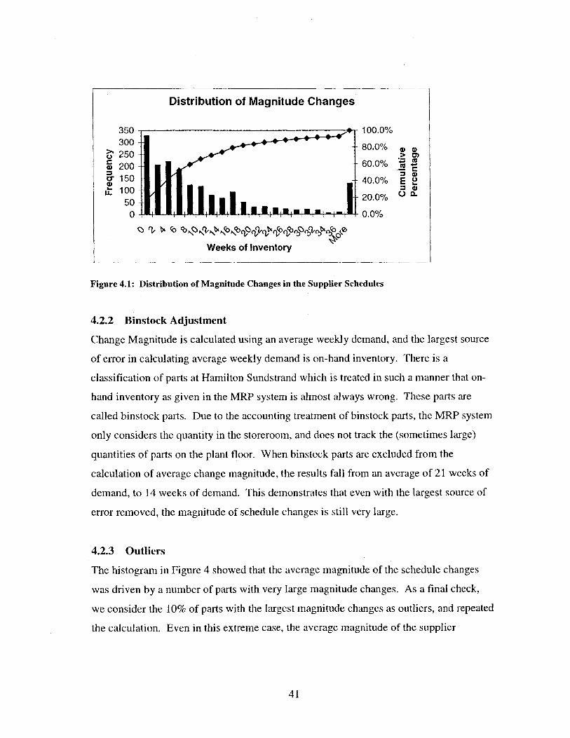
In order to better understand this result, we looked at the distribution of average
magnitude change for all the parts. Figure 4.1 shows a histogram of average magnitude
change. The vertical axis on the left side of the chart applies to the bar chart and shows
the number of parts (out of all 2000 parts) where the average magnitude change was
between zero and two weeks for the first column, between 2 and 4 weeks for the second
column, and so forth. The vertical axis on the right side of the chart applies to the line
graph, and shows the cumulative percentage of all parts. For example, 50% of all the
parts had a schedule change magnitude of 6 weeks or less.
It seems evident that the changes are indeed very large, but the average magnitude
change of 21 weeks given above is driven by several very large quantities. Since the
magnitude of change is calculated using an average weekly demand, and average weekly
demand is subject to large sources of uncertainty (refer to the Appendix for more
information), we felt further examination was necessary to better understand this
calculation.
40
Page 41
Distribution of Magnitude Changes
350 100.0%
300 80.0% 0o 250 >w 200 -- 60.0%
150 40.0% E- 10 20.0%
Weeks of Inventory
Figure 4.1: Distribution of Magnitude Changes in the Supplier Schedules
4.2.2 Binstock Adjustment
Change Magnitude is calculated using an average weekly demand, and the largest source
of error in calculating average weekly demand is on-hand inventory. There is a
classification of parts at Hamilton Sundstrand which is treated in such a manner that on-
hand inventory as given in the MRP system is almost always wrong. These parts are
called binstock parts. Due to the accounting treatment of binstock parts, the MRP system
only considers the quantity in the storeroom, and does not track the (sometimes large)
quantities of parts on the plant floor. When binstock parts are excluded from the
calculation of average change magnitude, the results fall from an average of 21 weeks of
demand, to 14 weeks of demand. This demonstrates that even with the largest source of
error removed, the magnitude of schedule changes is still very large.
4.2.3 Outliers
The histogram in Figure 4 showed that the average magnitude of the schedule changes
was driven by a number of parts with very large magnitude changes. As a final check,
we consider the 10% of parts with the largest magnitude changes as outliers, and repeated
the calculation. Even in this extreme case, the average magnitude of the supplier
41
Page 42
schedule change was seven weeks of demand. For a supplier with one month of safety
stock, such a change could easily deplete their inventory.
4.3 Volatility Amplification
It is clear that the supplier schedules show frequent changes, and that the magnitudes of
the changes are extremely large. This section will demonstrate how lotting policies work
to amplify the magnitude of changes in the MRP system. We repeat the volatility
analysis on the discrete demand schedule and show how the difference in results between
the discrete demand schedule and the supplier schedule is attributable to lotting policies.
4.3.1 Discrete Demand Results
The discrete demand schedule is the schedule of requirements used internally by buyers
and expeditors in the purchasing department. This schedule more closely represents the
actual internal demand for purchased parts. The supplier schedule is created from the
discrete demand schedule by the MRP system through the application of lotting policies.
The lotting policy is in turn dependent on a strata code. Each part in the system is given a
strata code, based on the annual dollar volume of usage. Higher dollar volume parts are
strata A or strata B, and are purchased in lots equal to one week of demand. Strata C
parts are much less expensive and are purchased in lots equal to eight weeks of demand.
Strata D parts are the most inexpensive parts, and are purchased in lots equal to 17 weeks
of demand.
An analysis of the discrete demand schedules for the same 2020 parts yielded the
following results:
> 86% of all parts had at least one schedule change
> On average there were 0.76 changes/part/week
> Average magnitude of change was equal to 6 weeks of demand
Comparing these results to the supplier schedule results shows:
42
Page 43
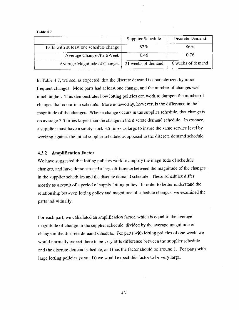
Table 4.7
Supplier Schedule Discrete Demand
Parts with at least one schedule change 82% 86%
Average Changes/Part/Week 0.46 0.76
Average Magnitude of Changes 21 weeks of demand 6 weeks of demand
In Table 4.7, we see, as expected, that the discrete demand is characterized by more
frequent changes. More parts had at least one change, and the number of changes was
much higher. This demonstrates how lotting policies can work to dampen the number of
changes that occur in a schedule. More noteworthy, however, is the difference in the
magnitude of the changes. When a change occurs in the supplier schedule, that change is
on average 3.5 times larger than the change in the discrete demand schedule. In essence,
a supplier must have a safety stock 3.5 times as large to insure the same service level by
working against the lotted supplier schedule as opposed to the discrete demand schedule.
4.3.2 Amplification Factor
We have suggested that lotting policies work to amplify the magnitude of schedule
changes, and have demonstrated a large difference between the magnitude of the changes
in the supplier schedules and the discrete demand schedule. These schedules differ
mostly as a result of a period of supply lotting policy. In order to better understand the
relationship between lotting policy and magnitude of schedule changes, we examined the
parts individually.
For each part, we calculated an amplification factor, which is equal to the average
magnitude of change in the supplier schedule, divided by the average magnitude of
change in the discrete demand schedule. For parts with lotting policies of one week, we
would normally expect there to be very little difference between the supplier schedule
and the discrete demand schedule, and thus the factor should be around 1. For parts with
large lotting policies (strata D) we would expect this factor to be very large.
43
Page 44
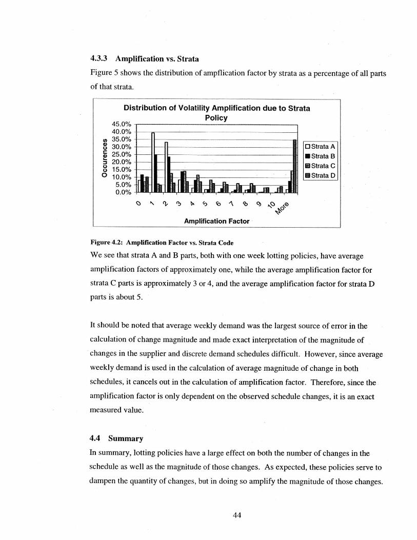
4.3.3 Amplification vs. Strata
Figure 5 shows the distribution of ampflication factor by strata as a percentage of all parts
of that strata.
Distribution of Volatility Amplification due to Strata
45.0%- Policy
40.0%U 35.0%8 30.0%- 0 Strata A5 25.0% N Strata B
20.0% * Strata Co 15.0%-0 10.0% E Strata D
5.0%0.0%
Amplification Factor
Figure 4.2: Amplification Factor vs. Strata Code
We see that strata A and B parts, both with one week lotting policies, have average
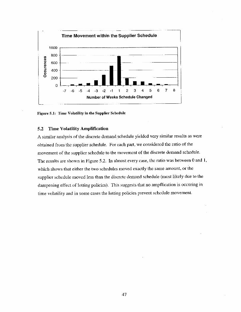
amplification factors of approximately one, while the average amplification factor for
strata C parts is approximately 3 or 4, and the average amplification factor for strata D
parts is about 5.
It should be noted that average weekly demand was the largest source of error in the
calculation of change magnitude and made exact interpretation of the magnitude of
changes in the supplier and discrete demand schedules difficult. However, since average
weekly demand is used in the calculation of average magnitude of change in both
schedules, it cancels out in the calculation of amplification factor. Therefore, since the
amplification factor is only dependent on the observed schedule changes, it is an exact
measured value.
4.4 Summary
In summary, lotting policies have a large effect on both the number of changes in the
schedule as well as the magnitude of those changes. As expected, these policies serve to
dampen the quantity of changes, but in doing so amplify the magnitude of those changes.
44
Page 45
This amplification factor was on average 3-4 for strata C parts and approximately 5 for
strata D parts. Therefore, small schedule changes can lead to very large schedule changes
at the supplier level. Furthermore, although we examined only the difference in the
discrete demand and supplier schedules, lotting policies are used throughout the MRP
system. It is not unusual for parts to be produced in batches of a fixed quantity or for the
plant to run batches of a particular part only one a month (i.e. period of supply lotting
equal to 4 weeks). Thus, there may exist an even larger amplification factor between
changes made at the customer level and the resulting change at the supplier level.
45
Page 46
5. Time Volatility Analysis
Having clearly identified how lotting policies can amplify the magnitude of a schedule
change, it may seem obvious that lotting policies will also cause changes to amplify in
time also. By time volatility, we mean movement of a requirement in time (for example a
part is required one week earlier than originally scheduled). This refers to all cases where
a demand already existed in the system and still exists after a change is made in the
system, but is scheduled for a different time.
Logically, it might seem likely that for a one week lotting policy, a change could cause
the lot to be needed as much as one week earlier or later. For an eight week lotting
policy, the change might be as large as plus or minus eight weeks. However, a careful
review of the fixed lot example in section 4 suggests no such phenomenon. In fact,
looking carefully at Tables 4.1 and 4.2, we see that a movement of the initial requirement
to one week earlier caused all schedules to adjust by exactly one week.
Using the analysis method described in the Appendix, we analyzed the time volatility of
the MRP schedule.
5.1 Analysis Results
Figure 5.1 shows the distribution of movement within the supplier schedule for the 2020
sample parts. The graph is a histogram of all the schedule changes which meet the time
volatility criteria outlined in the appendix. This represents all of the clearly identifiable
requirement movements in the schedule. It is apparent that most movements are about
two weeks, i.e. either parts are needed two weeks earlier or two weeks later. On average,
parts are needed later as often as they are need earlier. That means it is just as likely that
a supplier will need to deliver parts before expected as it is that they will need to hold
parts longer than expected.
46
Page 47
Time Movement within the Supplier Schedule
1000
800
600
8 4000 200
08-7 -6 -5 -4 -3 -2 -1 1 2 3 4 5 6 7
Number of Weeks Schedule Changed
Figure 5.1: Time Volatility in the Supplier Schedule
5.2 Time Volatility Amplification
A similar analysis of the discrete demand schedule yielded very similar results as were
obtained from the supplier schedule. For each part, we considered the ratio of the
movement of the supplier schedule to the movement of the discrete demand schedule.
The results are shown in Figure 5.2. In almost every case, the ratio was between 0 and 1,
which shows that either the two schedules moved exactly the same amount, or the
supplier schedule moved less than the discrete demand schedule (most likely due to the
dampening effect of lotting policies). This suggests that no ampflication is occuring in
time volatility and in some cases the lotting policies prevent schedule movement.
47
-M
Page 48
Time Volatility Amplification vs. Strata Code
80.00%-c 70.00%-
S60.00% -0 Strata AU) 50.00%-.0 U Strata B
40.00% * Strata Ce 30.00%20.00% U Strata D
0- 10.00%0.00%
-7 -6 -5 -4 -3 -2 -1 0 1 2 3 4 5 6 7 8
Time Volatility Amplification Factor
Figure 5.2: Time Volatility Amplification versus Part Strata
5.3 Summary
It is clear that the supplier schedules show frequent changes, and that the magnitude of
the quantity change is amplified by the lotting policies. A further analysis of the effect of
lotting policies on schedule volatility suggests that time volatility is not amplified in the
same manner, and that in this case lotting policies are useful in dampening the volatility
in the MRP schedule.
48
Page 49
6. Proposals for Reducing Schedule Volatility
We have shown how lotting policies amplify the magnitude of schedule changes.
Although the purchase part schedule used internally (discrete demand) shows average
magnitude changes equal to approximately six weeks of average demand, the schedule
that the suppliers work to shows magnitude changes 3.5 times larger. The suppliers,
lacking any other information, naturally assume that Hamilton Sundstrand is making
large, frequent schedule changes.
This section will suggest several methods for reducing the effects of MRP volatility
amplification by discussing alternate methods of communicating requirements to
suppliers as well as alternate methods of planning and ordering parts. The effect of
alternate planning and ordering methods on supply chain inventory will also be
discussed.
6.1 Supplier Communication
One of the primary reasons that two different schedules exist for purchased parts is a
desire to reduce the work load on internal buyers. Traditionally, buyers had to issue
purchase orders for every demand. They would take the recommendation from the MRP
system and manually issue a PO to the proper supplier for each part. This effort could be
considered a set-up time. For inexpensive parts, the cost of this "set-up" time was large
compared to the cost of the parts, and therefore it made sense to issue POs for large
quantities of inexpensive parts. In essence, a large batch size is required to justify the set-
up cost. This logic led to the creation of strata policies to automatically determine the
economical lot size for a given cost part.
As computing power grew, it became economical to automate the task of producing
purchase orders. Suppliers signed long-term agreements to ship parts at specific prices
over an extended period of time, and were issued requirements schedules automatically
by EDI or, more recently, over the internet. This significantly reduced the work load on
the buyers. In the process, the manual review which occurred before the PO was issued
was replaced by an automatic lotting logic within the MRP system. A side-effect of this
49
Page 50
change was the fact that suppliers now see very large levels of schedule volatility, as the
computer now makes changes based on mathematical principles, without the benefit of a
manual review. Whereas a buyer might choose not to make a change to a supplier's
schedule because of a small change in discrete demand, tacitly recognizing that the
change is not worth the confusion it might cause, the computer now makes the change
automatically. One way to reduce the impact of this side-effect is to change the way
schedules are communicated to suppliers.
6.1.1 Discrete Demand
Under the current system, the only information a supplier receives regarding future
demand comes from the supplier schedule. Due to the effects of MRP amplification, this
schedule is subject to very large changes in quantities from week to week. In addition,
this schedule does not accurately reflect the actual timing of demand for the part.
Although the lotting policies were created as a recognition of high internal "set-up" costs
associated with purchasing parts, such as buyers preparing and sending purchase orders,
the receiving department manually unloading, entering, and stocking shipments, and the
business office manually sending invoices, the majority of these processes have been
automated. Although there are production and transportation economies of scale for the
supplier, the need for Hamilton Sundstrand to place orders in large lots is very small.
Unfortunately, by sending suppliers a schedule with a lotting policy applied, Hamilton
Sundstrand is in fact partially dictating a batch size for the supplier. The lotted schedule
may call for 1700 parts every 17 weeks, leading the supplier to produce a batch of 1700
parts schedule for completion just prior to the expected need date. If the date and
quantity suddenly change, it may be very difficult for the supplier to adjust their
production schedule.
Consider an alternative where the supplier receives the discrete demand schedule for
planning purposes, but is given the option to ship up to a 17 week lot size of parts. In this
case, the schedule may call for 100 parts each week. The supplier determines his own
internal economic batch size and chooses to make batches of 500. Since the batch size is
50
Page 51
not too large, he is more willing to hold the parts in inventory, recognizing that the
likelihood is very high that all 500 pieces will be consumed. He therefore produces the
parts ahead of schedule to assure he can handle the inevitable change. When the time
comes to ship the first 100 pieces, the supplier sees that he is permitted to ship 1700
pieces. He sends the 500 pieces he produced, recognizing that this will erase all
scheduled requirements for the next 5 weeks, and that the next schedule he will receive
should reflect this change. Based on this, he plans the next production of 500 pieces. If
for some reason, the schedule changes, he may elect to still complete the lot of 500
pieces, confident that when he does need to ship the parts, he will be able to ship both lots
based on a maximum permissible shipment of 17 weeks worth of demand
In essence, we are giving the supplier access to a less volatile schedule that more closely
reflects the actual demand for the part, allowing him to make his own decisions regarding
what batch sizes are most economic for him to produce and ship. In addition, since both
schedules are currently created, there is relatively little effort required to implement this
proposal.
6.1.2 Customer Demand
Although this thesis focuses mainly on lotting policies applied to the purchased part
schedules, in reality lotting is applied at every level of the bill of materials and to
transfers of parts between plants within Hamilton Sundstrand. Therefore, it is reasonable
to expect that providing suppliers with schedules of actual customer demand would
provide similar benefits to that obtained by switching from the lotted supplier schedule to
the discrete demand schedule.
Attractive as this suggestion may seem, in reality it may be very difficult to implement.
There are many factors used to generate a schedule for purchased parts from the
corresponding customer demand. These factors may include the number of parts per end
assembly from the BOM, maufacturing lead-times, demand for subassemblies and
purchased parts from spares customers in addition to end item demand from OEM
customers, impact of loss and scrap, and many other factors. Many of these parameters
51
Page 52
are dynamically changing, making it difficult to simply provide a schedule of customer
demand to suppliers for planning purposes. In addition, internal lotting for batch
processes can cause a mismatch in the timing of shipments from suppliers and customer
demand. Take for example an item with constand customer demand of one/week. If a
subassembly requires a batch process with lot size of ten, all ten parts must be received
from the supplier simultaneously to cover the next ten weeks of customer demand.
Although we might expect that linking suppliers to end item demand is desirable in
reducing schedule volatility, there is no mechanism in MRP which allows such a linkage
to easily be provided. However, it is worth mentioning that very successful pull systems
actually link production of the lowest levels in the BOM to end item demand. Although
we will not discuss the design of pull systems in create detail in this thesis, two pull
systems that have been discussed at length in the academic literature that do link end item
demand to the early manufacturing operations include CONstant Work In Process
(CONWIP) systems and Hybrid systems.
A CONWIP system is one in which the total inventory (including work in process and
finished goods) is maintained at a constant level by sending a signal to the first operation
to start producing a part immediately after a part is removed from finished goods
inventory. This part is then "pushed" through subsequent manufacturing steps. A hybrid
system usually combines a CONWIP system with individual pull signals from the various
manufacturing steps in the process to the previous operations. In this case, inventory is
maintained at a constant level and parts are "pulled" from one operation to the next. The
next section will suggest how such production systems may be used to reduce schedule
volatility.
6.2 Alternate Order Policies
Throughout the duration of this research, Hamilton Sundstrand was considering alternate
ordering policies to reduce the schedule volatility problem and reduce inventory levels.
The methods under consideration included using production planners to manually create
fixed, level loaded schedules for suppliers, and implementing a pull system. The pull
52
Page 53
system could be implemented either just at the purchased part level, using MIRP to
simulate a two bin system and automatically send a Kanban card to the supplier when one
bin went empty, or it could be integrated throughout the manufacturing process so that
the purchased part demand was driven by end customer demand. In addition, we will
discuss how ordering parts in smaller lot sizes may be used to decrease schedule
volatility.
This section discusses the advantages and disadvantages to each alternative approach in
the areas of quantity and time volatility and the amount of manual intervention required.
The next section will discuss some theoretical aspects regarding inventory under each of
these systems.
6.2.1 Reduced Lot Sizes
Historically, Hamilton Sundstrand used large lot sizes for ordering inexpensive parts due
to the many fixed costs associated with handling each order. Although automated
processes have replaced many of the manual processes which led to these high fixed
costs, the lotting policies remain essentially unchanged. Actually, Strata policy specified
weekly ordering for Strata A parts, monthly for Strata B parts, semi-annually for Strata C,
and annually for Strata D. About three years ago, Hamilton reduced the lot sizes to their
current values in order to reduce inventory in the plant.
Even with the decrease in lot sizes, replacing manual order placement with MRP lotting
logic led to amplification of schedule volatility from the point of view of suppliers. This
amplification increases with increased lot size. For these reasons, it might make sense to
reduce the lot sizes even further. With no changes to the current system, reducing lot
sizes should improve the amplification factor and thereby reduce the magnitude of the
quantity volatility seen by suppliers. However, even with smaller lot sizes, suppliers will
be exposed to volatility both in the magnitude and the required date of shipments.
53
Page 54
6.2.2 Fixed, Level Loaded Schedule
During the period this research was conducted, there was tremendous pressure to improve
supplier delivery performance. Since suppliers felt that schedule volatility was the
largest factor affecting their on-time delivery metrics, the suggestion was made to
provide suppliers with a fixed schedule, preferably for a fixed quantity per time period.
The idea was to take parts that were primarily used in OEM customer parts (for example
the Boeing 777 is a relatively new aircraft and is almost entirely OEM demand, with very
few spare parts requirements), have a planner determine a fixed schedule for the parts,
and communicate this schedule to the suppliers. For example, even if the demand from
Boeing was not entirely level, the planner would determine the total demand over a long
period, and have the supplier produce x parts per month.
The advantages to such a proposal are: Suppliers get an absolutely fixed schedule with
no time or quantity volatility - unless the planner did not account for any of a number of
unforeseen events. Not only would such a policy only work on a percentage of all
purchased parts (those used primarily in OEM parts), but it would require a huge effort
on the part of the planners. The MRP system was implemented to prevent this effort! In
addition, if demand grows over and above the schedule initially provided to suppliers
(due to scrap, loss, change in customer demand, etc.), it may be very difficult to get
additional parts. The supplier, believing he is working to an absolutely fixed schedule,
may have no additional raw material on hand to support the new demand. This may be
especially problematic if the raw material includes long lead-time items like castings or
forgings. This problem can only be avoided by increased effort in planning or by
increased safety stock. Both may be very expensive and Hamilton, by removing all
volatility from the suppliers, would in essence be carrying all of the cost and risk
associated with the reduction in schedule volatility.
6.2.3 Pull System
An ongoing subject of discussion at Hamilton Sundstrand deals with the practicality of
using a pull system. The opposition to such a system centers around the general high
product variety, low quantity production of aerospace parts in general, and the high
54
Page 55
unpredictability of spares demand in particular. Many people within the company
believe that a pull system will only lead to increased inventory of purchased parts in the
plant, due to the large number of partially filled bins scattered throughout the factory.
Sundstrand began using pull systems with their suppliers many years ago, apparently
with good success. After the merger with Hamilton, and the subsequent need to
standardize and replace the Sundstrand legacy computer systems with the J.D. Edwards
system used at Hamilton, functionality within the MRP system was added to duplicate the
pull system used by Sundstrand. It is interesting to note that overall, Sundstrand has
considerably higher on-time delivery performance from their pull system suppliers, but in
general has more on-hand inventory than Hamilton.
In most cases, Sundstrand uses a two bin system with an automatically generated pull
system. This means that a bin size is defined, and if the on-hand inventory level falls
below this bin size, the computer automatically sends out an email to the supplier to send
a bin size worth of parts. The bin size is generally agreed upon with the supplier and
based on a production quantity that is economical for them to produce and ship.
Opponents to the pull system maintain that this system just replaces the current lotting
policy with a different, fixed quantity lotting policy. In fact, this change alone has a big
impact on schedule volatility. Steele (1975) suggests that using a fixed order quantity as
opposed to periods of supply can reduce volatility.
In addition, there may be some benefit to using a pull system in the area of smaller lot
sizes, since one might generally expect the bin sizes to be smaller than 8 or 17 weeks of
average demand.
Furthermore, the fact that the MRP system is not attempting to maintain inventory at zero
by planning orders to arrive when inventory drops to nothing, but instead places an order
when on-hand inventory falls below one bin, represents a form of safety stock. Many
55
Page 56
authors including Kropp (1979), suggest that safety stock can be used to dampen
schedule volatility.
Finally, there is a benefit to the supplier in that there is only time volatility and no
quantity volatility. If the bin size (or lot size) is 50 pieces, than the requirement will
always be for 50 pieces (or 100 pieces if both bins are emptied simultaneously).
Therefore, the only variability in the schedule is the timing. As we have demonstrated,
there is no time volatility ampflication within the MRP system, and the average time
volatility is two weeks. This means that on average, the 50 pieces will be required within
a period two weeks sooner or two weeks later than originally expected. Based on this
knowledge, a supplier would need only produce the 50 pieces two or three weeks earlier
than expected, and still be able to meet most schedule changes.
A disadvantage to the pull system lies in the increased effort needed to maintain this
system. Bin sizes must be manually sized, and periodically reviewed. If demand for a
part decreases, due to a reduction in customer demand, or an engineering change which
renders the part obsolete, this may need to be manually accounted for, so that Hamilton
Sundstrand is not left holding two bins of unusable inventory.
6.2.4 Pull System linked to Customer Demand
In section 6.2.3., we assumed a pull system in which the MRP system is used to plan all
work orders, and then automatically plans and places orders for purchased parts with
suppliers as necessary to maintain the on-hand inventory. This means that the purchased
part demand alone drives the orders to suppliers. Consider the example in section 4.1.1.
in which customer demand for the end item "abc" was perfectly level at two units a week,
but the purchased part "xyz" was consumed in groups of twelve due to lotting policies
within the MRP system for higher assemblies. Although an economical lot size for the
supplier might be less than twelve units, he would be constrained to deliver at least
twelve each delivery. If he wished to produce in lots of eight pieces, he would need to
deliver at least two lots to satisfy the demand. In essence, the MRP system's internal
56
Page 57
lotting policies create a practical limit to how small the lot sizes can go before they are no
longer effective in reducing schedule volatility.
In fact, an examination of the discrete demand schedule suggests that the maximum
demand in one week is approximately eight to twelve times the average weekly demand
for the part, suggesting that MRP lotting policies "lump" purchase part demand into lots
of two to three months before any lotting policy is applied to the supplier schedule. The
results of the discrete demand schedule analysis, which demonstrate that the average
magnitude change represents four to six weeks of average usage further substantiates this
idea.
If we accept that the work order lotting policies used by the MRP system are valid, can
we develop a system which still allows suppliers to ship smaller lots on a more regular
basis? For example, if suppliers could make weekly shipments of small, fixed lots, we
would expect this to eliminate quantity volatility (through the use of fixed lot sizes), and
also reduce time volatility from the current level of approximately plus or minus two
weeks.
xvz buffer mm, cner uvw buffer def ooer. def buffer abc assm. fin. Inv.
Figure 6. 1 CONWIP Manufacturing System
Consider a CONWIP (CONstant Work In Process) manufacturing system used with the
example from 4.1.1. Such a manufacturing system is diagrammed in Figure 6.1. The
circles represent assembly or manufacturing operations and the triangles represent buffer
inventory. When one end item is taken from the finished goods inventory buffer, a signal
is sent to the supplier to deliver a part. Since assembly "uvw" is produced in lots of
twelve, the buffer in front of this operation is allowed to accumulate
57
Page 58
parts so that when the operation is ready to be performed, twelve parts are in the buffer.
Consider the schedule for purchased part "xyz" under the original system, with constant
demand for "abc" of two per week, and a fixed lot size of 12 pieces for "uvw". Also
consider the schedule for part "xyz" under the CONWIP system:
Table 6.1
Overdue Wk I Wk 2 Wk 3 Wk 4 Wk 5 Wk 6 Wk 7 Wk 8
Item "abc" 2 2 2 2 2 2 2 2 2
Ass. "uvw" 12 0 0 0 0 12 0 0 0
"xyz" with 12 0 0 0 0 12 0 0 0
MRP
"xyz" with 2 2 2 2 2 2 2 2 2
CONWIP
By linking the purchased part demand with the demand for the end item, we would
expect a reduction in MRP generated quantity volatility amplification. In addition, the
supplier is now able to further reduce his lot sizes.
A problem with this system, in addition to the need to manually plan and track bin sizes,
is the difficulty in aggregating demand. Since a purchased part may be used in multiple
end items, may be required to satisfy replacement part demand for a subassembly, or may
be needed to replace scrapped parts, it is difficult to ensure all demand has been
communicated to the supplier. It may be desirable to separate spares and OEM demand
for a given purchased part and implement an additional pull signal for scrapped parts.
6.3 Inventory Considerations
Throughout section 6.2, several alternate planning and ordering policies were suggested
to reduce schedule volatility. Since the MRP system generates volatility due to the
manner in which it attempts to exactly plan orders and production so as to minimize
inventory, we might expect these solutions to impact inventory levels within the supply
chain. Since a primary concern of Hamilton Sundstrand is the reduction of inventory, the
impact on inventory levels is very important. In this section, we will discuss some of the
effects of these planning and ordering policies on inventory levels.
58
Page 59
Although this analysis is not intended to be rigorous, it should give an idea of order of
magnitude levels. For the sake of this discussion, we will assume that end items are
produced in weekly lot sizes (approximately steady demand) and that the lowest level sub
items, and therefore the purchased parts, are produced every six weeks, due to the MRP
internal lotting policies.
6.3.1 Current MRP System
Purchase Part Inventory - Hamilton Sundstrand
The amount of inventory for purchased parts, assuming 100% supplier delivery, is
dependent on the relative size between the shipment lot size and the demand lot sizes.
Figure 6.2 shows on-hand inventory levels under two different conditions. The graph on
the right assumes perfectly steady consumption, with a lot size of 17 weeks. This means
that a supplier delivers 17 weeks worth of parts, which are consumed in small quantities
steadily throughout the next 17 weeks. In this case, average inventory is equal to the area
under the graph, or one-half of 17 weeks = 8.5 weeks.
Inventory with Shipment Sizes equal to Inventory w ith Steady Dem andDemand Lots
18
5 106_
1 -- - _ 1- -_ _
02
010 1510 5 10 10
Week We
Figure 6. 2 Inventory Level with the MRP system
The graph on the left assumes that the supplier ships in lots of four weeks, and that the
parts are immediately used in the lowest level assembly, which are also built in lots of
four weeks. In other words, the shipment lot size = demand lot size. In this case the
average on-hand inventory is very nearly zero. While these examples represent extreme
cases, we see that inventory levels are constrained between zero and one-half the
shipment lot size. Since Strata A and B parts currently use a period of supply lotting
59
Page 60
policy of one week, we would expect inventory of Strata A and B parts to be very close
to zero. For Strata C parts, with a lot size of 8 weeks, if we assume that the lowest level
assemblies are produced only once every six weeks, then inventory of Strata C parts
should also be close to zero. Strata D parts, with lot sizes of 17 weeks, would have an
average on-hand inventory approximately 8 weeks, however, since these parts are very
low dollar value, this inventory should be negligible from a monetary standpoint.
Although Hamilton Sundstrand is able to maintain very low inventory of purchased parts
under this scenario, the supplier is not as lucky. He sees a schedule characterized by
frequent, large schedule changes, with an average change representing perhaps eight to
twelve weeks of inventory. Faced with this environment, he can decide to carry a large
amount of inventory on his shelves, or attempt to expedite orders to meet changes. If we
refer to the histogram showing the distribution of magnitude changes in the supplier
schedule (Figure 4.1), we see that the supplier would need to hold 30 weeks of inventory
in order to meet 90% of all schedule changes. Even a 75% service level would require
inventory levels of 16 weeks.
Furthermore, if the supplier, unwilling to carry such large amounts of inventory does
suffer from poor delivery performance, Hamilton Sundstrand would expect to see rising
levels of inventory, as WIP and purchased part inventory increase because product can
not be built in a timely fashion, customer delivery performance falls, and Hamilton
Sundstrand reacts by increasing system lead-times and safety stock levels. In fact, this is
exactly what is happening.
6.3.2 Fixed, Level Loaded Schedule
In this case, the MRP system has been replaced with a human planner, who examines the
schedule and communicates a fixed, preferably constant demand schedule to the supplier.
This relieves the supplier of any uncertainty in demand, and he responds by reducing his
inventory of finished goods to essentially zero, as he attempts to complete parts exactly
when they are needed by Hamilton Sundstrand, and only carries the parts in inventory if
he completes them sooner than expected.
60
Page 61
Having a person plan the deliveries of purchased parts, however, does nothing to address
the causes or amplification of schedule volatility, and therefore, Hamilton Sundstrand
must carry a large safety stock of inventory to deal with schedule changes. The discrete
demand schedule has magnitude changes on average equal to six weeks of inventory.
However, since the supplier may have very limited ability to react to changes, Hamilton
may need to use a buffer larger than 6 weeks. In fact, if Hamilton Sundstrand wanted to
size the buffer to handle 90% of all changes, the buffer would need to be set at 8 weeks of
inventory. At 95%, a buffer of 15 weeks of inventory would be needed.
Finally, a potential mismatch in timing of supplier delivery and actual consumption may
exist. For example, Hamilton Sundstrand might need 50 pieces at the end of May, but the
supplier is scheduled to deliver parts at the beginning of every month, causing the parts to
sit in inventory for the entire month. Also, if the schedule is not examined on a regular
basis, a situation may occur where decreasing demand for a part is not matched by
decreasing shipments from the supplier, further increasing inventory levels.
Although this analysis is not intended to be rigorous, it is reasonable to assume that there
is a trade-off between manual planning effort and inventory level in this system. One
reason that MRP systems were created is because such manual planning efforts are very
difficult, and often result in poor service levels and high inventory levels. Although the
advantage to the suppliers is clear, in the long-run, it seems likely that such a manual
system would be abandoned for MRP planning once again.
6.3.3 Pull System
A significant source of resistance to the implementation of a pull system manufacturing
process revolves around the concern that such a system will dramatically increase the
inventory levels as compared to the current MRP system. In order to answer this
concern, let us consider two ideal cases. For the first case, assume that the time required
by the supplier to refill an empty bin (replenishment time) is small compared to the
consumption of parts. For example, assume that the lowest level assembly is produced
61
Page 62
0 2 4 6 8 10 0 0.5 1 1.5 2 2.5 3
Week Replenishment Periods
Figure 6. 3 On-Hand Inventory in a Pull System
monthly, and that the supplier can refill the bins immediately. Also assume that when the
consumption occurs, a quantity greater than one bin but less than or equal to two bins is
used, thereby triggering a signal to refill the bins. For the second case, assume that
consumption is perfectly steady, and the bin size is set exactly equal to the consumption
during the replenishment time. Figure 6.3. shows the inventory levels under both of these
perfect scenarios.
In the first case, average on-hand inventory is very nearly equal to two full bins. In the
second case, the average on-hand inventory is equal to half of a bin. Since these two
cases represent opposite, ideal situations, we would expect to find that inventory levels
are somewhere in between these cases. In addition, since many of the suppliers that
Hamilton Sundstrand uses are within several hours of the plant, and since demand for
lower level items occurs only every few weeks (partly due to internal MRP lotting
policies), we would expect inventory levels to more closely approximate the first case.
Typically, Hamilton Sundstrand uses the logic that the bin size should be set equal to the
largest demand within the replenishment time. Therefore, if the replenishment time is
one week, the largest single week of demand would be used to size the bin. For this
analysis, we are assuming that the low level items are consumed all at once in a quantity
equal to six weeks of demand, and therefore the bin size would be set equal to six weeks
for any replenishment time of six weeks or less (replenishment time would almost always
be less than two weeks, except for very distant suppliers). Therefore, we would expect
62
Replenishment Time <<ConsumptionInterval
2
1.5
=1IL
0.5
(1
Steady Consumption compared toReplenishment Time
2
1.5
0.5
0
---- --------------------------
----- -------- ----------- -----
- ---- - --- - - -- - - - -- - -- ---- --
Page 63
average on-hand inventory under a pull system to be approximately two bins of six weeks
each, or twelve weeks of inventory.
In addition, the supplier would be expected to carry inventory to account for schedule
volatility. He is now no longer buffering against quantity volatility, since he is shipping
fixed quantity lot sizes, and expects to receive the actual pull signal two weeks before or
after originally expected. Since he receives the pull signal on average once every six
weeks, he might just adopt a policy of always keeping one bin worth of parts on-hand.
This amounts to an additional inventory of one bin (six weeks) over and above the twelve
weeks carried by Hamilton Sundstrand.
6.3.4 Pull System linked to Customer Demand
In this scenario, we apply the same logic that we used to analyze the pull system at the
purchased part level in section 6.3.3. We will assume that most suppliers are located in
the general geographic area of the plant, and therefore replenishment time is generally
one to two weeks. Furtheremore, we will use Hamilton Sundstrand's bin sizing logic in
which the bin size is set to the largest demand during replenishment time. However, now
we will assume that the purchased part pull signal is driven by end item demand.
For this analysis, we assume that end item demand is fairly steady, with very nearly the
same quantity produced each week. Since purchased part demand is now driven by end
item demand, the purchased part usage is fairly steady also. We might reasonably expect
this scenario to more closely resemble the second case shown in Figure 6.3. In this case,
on-hand inventory levels were maintained at one-half of a bin. Unfortunately, even in
this case, demand is not completely steady, and is about the same order of magnitude as
replenishment time. I.e., parts are consumed once a week, and the supplier takes several
days to refill the bin. Therefore, it might be more reasonable to assume that on-hand
inventory is approximately one bin.
Using the same logic to determine the bin size, we conclude that the bin size should be
set equal to the largest demand during replenishment time, or between one and two weeks
63
Page 64
of demand. Therefore, we conclude that the on-hand inventory is approximately one bin,
of one to two weeks inventory. Furthermore, the supplier also carries an extra bin on-
hand to guard against schedule volatility, resulting in a total supply chain inventory level
of two to four weeks of inventory.
6.4 Summary
Table 6.1. summarizes the advantages and disadvantages of each ordering policy in the
area of schedule volatility (both quantity and time), manual planning effort required, and
inventory levels.
Table 6.2
Schedule Volatility Planning Effort Inventory Level
Quantity Time Upfront Ongoing Supplier HS
Current System High Yes None Low 16-30 wks -0 wks
Fixed Schedule None None High High -0 wks 8-15 wks
Pull System None Yes Medium Low 6 wks 12 wks
CONWIP/Hybrid None Yes Medium Low/Med 1-2 wks 1-2 wks
From the table, we can see that there is a cost to reducing schedule volatility, either in
increased manual effort, or in increased inventory levels at Hamilton Sundstrand.
However, it should be noted that although the theoretical Hamilton Sundstrand inventory
levels for the current system are very small, actual inventory levels are much higher.
This is partially due to current efforts to combat poor supplier deliver, generally in the
form of lead-time or inventory buffers. Furthermore, although any of the alternate
planning methods would likely increase the inventory levels at Hamilton Sundstrand, the
actual total supply chain inventory would likely decrease. Hamilton Sundstrand must
therefore determine if the disadvantage to carrying the inventory on their books is
outweighed by the benefit of an overall reduction costs through the reduction in overall
supply chain inventory levels.
Furthermore, we should note the fact that suppliers do not carry such high levels of
inventory under the current system is reflected in the poor supplier delivery performance,
64
Page 65
and therefore we would expect any of the alternate proposals to improve delivery
performance. In fact, former Sundstrand sites that use Pull Systems do have generally
higher levels of inventory, but also have vastly better supplier deliver performance.
65
Page 66
7. Recommendations and Conclusions
The analysis of schedule volatility has shown that supplier schedules are characterized by
frequent, large magnitude changes. Although these changes are driven by changes in
customer demand, as well as changes made within Hamilton Sundstrand at all levels of
the MRP system, these changes are amplified in magnitude by period of supply lotting
policies used to create the Supplier Schedule. A supplier wishing to achieve a 90%
service level in this environment without constantly adjusting his production plan would
need to carry 30 weeks of inventory for each part to insure he could accommodate the
changes.
The fact that suppliers may be unwilling or unable to carry such large amounts of
inventory is evidenced by their poor on-time delivery performance and the high level of
WIP inventory at Hamilton Sundstrand that cannot be completed until remaining parts
arrive from suppliers.
There are several ways in which schedule volatility can be reduced, including reducing
changes at their source. Unfortunately, these efforts have historically proven difficult and
ineffective. The amplifying effect of the MRP system can be reduced in a number of
ways, including reducing lot sizes, changing the way schedules are communicated to
suppliers, or by adopting fixed lot sizes, preferably in the form of a pull system.
Recognizing that many of these recommendations take time to implement, and
understanding that the problem needs to be addressed immediately in some manner, we
have divided these recommendations into three groups, based on implementation time.
7.1 Reduce Lot Sizes, Use Fix Lot Sizes and Work to Discrete Demand
The easiest and quickest solution is to reduce lot sizes and/or switch to a fixed lot size
policy. Reducing lot sizes while maintaining a period of supply policy will help reduce
the amplifying effect of the MRP system, thereby decreasing the magnitude of schedule
changes that the supplier sees. Although this change will in general increase the number
of changes a supplier sees each week, he will be able to accommodate schedule changes
66
Page 67
with lower inventory levels. In other words, he may see more schedule changes each
week, but will be more likely to be have parts in inventory when a change occurs, thus
increasing his on-time delivery performance.
Many suppliers have minimum order size requirements, however, these should not be
impacted by reducing the lot sizes. The MRP system already contains logic that places
orders based on the larger of either the minimum order size or the lotted order size. For
suppliers who have not traditionally specified a minimum order size, and now find
themselves sending parts more frequently than is economical, minimum order sizes can
be entered at any time, and the planned orders will be adjusted accordingly.
Furthermore, recognizing that the use of fixed lot size ordering itself will reduce schedule
volatility, it may be desirable to work with individual suppliers to identify economical
order sizes. These lot sizes should generally be less than or equal to the average order
size under the current period of supply lotting system to prevent an increase in inventory
levels at Hamilton Sundstrand. The supplier will now expect orders in multiples of this
fixed lot size, and can plan his production accordingly.
Although the fixed lot size is very effective in reducing schedule volatility, the possibility
exists that Hamilton Sundstrand will occassionaly purchase more parts than are really
needed to meet future demand. For example, if the fixed lot size was 10 pieces, and
Hamilton Sundstrand had a requirement for 1 piece, with nothing else in the future, the
RP system would place an order for 10 pieces, leaving the plant with 9 unneeded parts.
To eliminate this problem, Hamilton Sundstrand can reduce schedule volatility without
changing lotting policies simply by communicating the discrete demand schedule to
suppliers, while still allowing them to ship any quantity less than or equal to the lotted
value. The supplier will work to a less volatile schedule that more closely matches the
actual demand for parts. In order to avoid confusion, the manner in which the discrete
demand schedule and the maximum allowable shipment quantity (based on the lotting
policy) are communicated should be discussed with suppliers.
67
Page 68
7.2 Pull System Manufacturing
Sundstrand, before their merger with Hamilton Standard, began using pull system
manufacturing. The result of this implementation was a marked increase in supplier
delivery performance. The smaller, fixed lot size ordering which characterizes this
system provides a much lower level of schedule volatility, resulting in lower required
supplier inventory and thereby improved service levels. The partially filled bins within
the plant serve as safety stock and also help to reduce schedule volatility by absorbing
schedule changes.
Purchased part inventory levels at Hamilton Sundstrand with a pull system are certainly
larger as compared to a perfectly functioning MRP system. However, poor supplier
delivery has led to high levels of partially completed WIP inventory and an increase in
lead-time and safety stock buffers, therefore, such a direct comparison of total inventory
in the plant is invalid. Furthermore, the resulting schedule stability allows suppliers to
significantly reduce inventory levels, and total supply chain inventory for the purchased
parts actually decreases under the pull system. Since Hamilton Sundstrand eventually
absorbs the supplier's inventory holding costs in the form of higher direct material
purchased cost, a pull system results in a net benefit.
In order to facilitate the introduction of the MIRP system used at Hamilton in the former
Sundstrand facilities, functionality has been created in the system to work with a pull
system. Therefore, this functionality can be used to order parts from suppliers on a pull
system, without significant changes within the factory. However, since placing parts on
a pull system requires that suppliers produce additional parts over and above the current
scheduled demand in order to intially fill the bins, this process should be discussed with
each supplier individually, and a schedule created to place parts on the system.
7.3 Pull System with CONWIP or Hybrid Control
Once suppliers begin working to a pull system, Hamilton Sundstrand should begin
working to reduce bin sizes, and thereby reduce the amount of inventory in the plant.
Although the ideal goal of single piece flow (lot sizes of one piece) may be uneconomical
68
Page 69
for supplier deliveries, the process of reducing bin sizes is still worthwhile. Many
suppliers deliver a wide range of part numbers, and Hamilton Sundstrand continues to
rationalize and reduce their supply base. Therefore, it may be possible for suppliers to
economically ship small lot sizes, since they are shipping many parts simultaneously.
Unfortunately, bin size is currently driven by demand lot size. There is little use in
having two bins, each with one piece, when the assembly that uses the part is always built
in lots of eight. Even with fairly even, steady customer demand at the end item level,
lotting policies at lower levels in the bill of materials force the purchased parts to be
consumed in larger lots than might otherwise be acceptable. However, by linking
purchase part pull signals to consumption of the end items, this aspect of the MRP system
can be circumvented. By placing a buffer in front of the batch operation, small lot sizes
can be ordered, while simultaneously allow processes which require batch operation to
run economically. In essence, the lower levels of the bill of materials have been
decoupled from the higher levels in a manner which is impossible to achieve with an
MRP system.
Hamilton Sundstrand has already begun considering pull systems which link all the
processes in the manufacturing of an end item to the demand of the end item. Termed
Supply Chain Integration, or SCI, such a system requires considerable work to design and
implement, but holds the promise of greatly reduced inventory levels and a simultaneous
decrease in schedule volatility.
7.4 Future Research
Considerable work has been done to demonstrate how quality improvments can be
obtained and inventory can be reduce through the use of pull system manufacturing. We
believe that such a system also presents considerable advantages in the area of schedule
stability. The fact that a formal schedule typically only exists for forecasting purposes in
traditional pull systems makes it difficult to actually measure schedule stability.
However, as companies try to adopt their MRP system to a pull system methodology, the
opportunity exists to study schedule stability improvements. Furthermore, modeling and
69
Page 70
simulation can be used to compare schedule stability under many scenarios. Researchers
including Blackburn (1986) and Ho (1989) have carried out such studies using different
lotting policies to understand the impact on schedule volatility. Such an analysis should
be expanded to study the performance of various types of pull systems.
7.5 Conclusions
Lotting policies in the MRP system can amplify schedule volatility in modern MRP
systems, so that even small changes in the master schedule can lead to very large
requirement changes in the supplier schedules. Such changes may make it difficult for
suppliers to meet shipment schedules, eventually disrupting the downstream
manufacturing processes.
Although efforts to reduce the sources of volatility in the system, namely changes made
to the schedules and to MRP system parameters, and reduction of scrap and loss are
certainly desirable, such efforts have usually proven unsuccessful in ultimately improving
schedule volatility. However, through reduction of lot sizes, improved schedule
communication using discrete demand and the use of fixed lotting policies, schedule
volatility can be significantly improved.
Finally, implementation of pull system manufacturing, through the automatic use of fixed
lot sizes (bin size) and inherent safety stock from inventory in bins throughout the plant,
can further improve schedule stability. Unfortunately, the use of a pull system in a
manufacturing environment with large product variety and low production volumes may
lead to an initial internal increase in purchase part inventory. However, the improvement
in schedule stability and supplier delivery performance should lead to a decrease in
overall supply chain inventory levels and possibly total inventory levels in the plant.
Furthermore, implementation of a CONWIP or hybrid pull system can eliminate the
tendency of the MRP system to unnecessarily lot lower level items (including purchased
parts) and allow further reductions in inventory.
70
Page 71
Bibliography
1. Arnold, J. R. T. (1991). Introduction to Materials Management, Prentice Hall,
Upper Saddle River, New Jersey, p. 97.
2. Blackburn, J. D., Kropp, D. H., Millen, R. A. (1986). "A Comparison of
Strategies to Dampen Nervousness in MRP Systems" Management Science, No. 4, April,pp. 413-429.
3. Ho, C. J. (1989). "Evaluating the Impact of Operating Environments on MRP
System Nervousness", International Journal ofProduction Research, Vol. 27, No. 7, pp.
1115-1135.
4. Hoag, T. A. (1999). "Schedule Stability at Pratt & Whitney" unpublished.
5. Kropp, D. H., Carlson, R.C., Jucker, J.V. (1979). "Use of Dynamic Lot-Sizing to
Avoid Nervousness in Material Requirements Planning Systems" Production &
Inventory Management, 3 qtr., pp. 49-57.
6. Mather, H. (1977). "Reschedule the Reschedules you just Rescheduled - Way of
Life for MRP?", Production and Inventory Management, 1 t Qtr., pp. 60-79.
7. Minifie, J. R, Davis, R. A. (1986). "Survey of MRP Nervousness Issues",
Production and Inventory Management, 3rd Qtr., pp. 111-119.
8. Nahmias, Steven (1997). Production and Operations Analysis, Irwin, Chicago,
Illinois, pp. 363-365.
9. Steele, D.C. (1975). "The Nervous MRP System: How to Do Battle" Production
& Inventory Management, 4 qtr., pp. 83-88.
71
Page 72
Appendix - Schedule Volatility Analysis Methods
The MRP system is run every Sunday. Therefore a new schedule is created only once a
week. For simplicity's sake, we limit our investigation of schedule volatility to all
requirements within an eight-week period from the date the schedule was created.
Generally speaking, volatility within this time frame is most disruptive to a supplier. The
suppliers typically have determined their production requirements and ordered raw
material and therefore changes within this time frame require some type of expediting.
By limiting the investigation to an eight week period, we mean that we consider only
those requirements on any given weekly schedule that occur within a period starting on
the date the schedule was created, through the next eight weeks. We then compare that
schedule to a schedule created one week later, and compare that schedule to the following
weeks schedule, and so forth. Any parts that are received during the week are netted off
the current schedule, from the earliest requirement date (starting with overdue
requirements), and this adjusted schedule is then compared to the following week's
schedule. In essence, we are comparing what a supplier would reasonably expect to see,
with what they actually see each week.
Counting Schedule Changes
Consider a typical schedule for a single part number:
Table 1
Overdue Wk I Wk 2 Wk 3 Wk 4 Wk 5 Wk 6 Wk 7 Wk 8
Schedule 1 0 0 0 10 0 15 0 24 0
The schedule shows the quantity required in each week for the next eight weeks. Since
the schedule was created Sunday, Wk 1 represents the need for parts from that Monday
until the end of the week and so on. The schedule also shows that there are no parts that
are overdue. If no changes occur which effect the schedule, the supplier would expect
the schedule on the following week to look like:
72
Page 73
Table 2
Overdue Wk1 Wk 2 Wk 3 Wk 4 Wk 5 Wk 6 Wk 7 Wk 8
Schedule 1 0 0 0 10 0 15 0 24 0
Schedule 2 0 0 10 0 15 0 24 0 6
If the supplier were to deliver 8 pieces during the week, they would expect the schedule
to become:
Table 3
Overdue Wk I Wk 2 Wk 3 Wk 4 Wk 5 Wk 6 Wk 7 Wk 8
Schedule 1 0 0 0 10 0 15 0 24 0
Schedule 2 0 0 10 0 15 0 24 0 6
Schedule 3 0 2 0 15 0 24 0 6 9
If the supplier makes no subsequent deliveries, the following week, 2 parts would be
overdue, as shown in the following schedule:
Table 4
Overdue Wk I Wk 2 Wk 3 Wk 4 Wk 5 Wk 6 Wk 7 Wk 8
Schedule 1 0 0 0 10 0 15 0. 24 0
Schedule 2 0 0 10 0 15 0 24 0 6
Schedule 3 0 2 0 15 0 24 0 6 9
Schedule 4 2 0 15 0 24 0 6 9 0
So far the schedule has been absolutely stable, with no signs of volatility. However,
suppose the supplier made no shipments, and the schedule next week looked like:
Table 5
Overdue Wk I Wk 2 Wk 3 Wk 4 Wk 5 Wk 6 Wk 7 Wk 8
Schedule 1 0 0 0 10 0 15 0 24 0
Schedule 2 0 0 10 0 15 0 24 0 6
Schedule 3 0 2 0 15 0 24 0 6 9
Schedule 4 2 0 15 0 24 0 6 9 0
Schedule 5 2 15 5 24 0 6 9 0 23
73
Page 74
The schedule now shows an additional requirement for five pieces. If the supplier now
delivers 20 pieces, he would expect the following schedule to appear the following week:
Table 6
Expected 0 2 24 0 6 9 0 23 0
This shows that the 20 pieces have been netted out from the earliest to the latest, so that
the two overdue pieces, the 15 pieces in week 1, and 3 of the 5 pieces in week 2 have
been satisfied. Suppose the schedule that week actually looked like this:
Table 7
Expected 0 2 24 0 6 9 0 23 0
Actual 0 4 24 0 6 9 0 23 0
The supplier expected a requirement of two pieces based on having shipped 20, but there
is now an open requirement for 4 pieces, an increase of two from what was expected.
It is worth noting that a pull-in of a requirement (i.e. an existing quantity is needed earlier
than originally scheduled) may be considered a single change by a human observer, but
would be counted as two changes - an increase in one weekly quantity, and a decrease in
a different week. For example:
Table 8
Schedule 1 0 0 0 0 20 0 0 0 0
Schedule 2 0 20 0 0 0 0 0 0 0
In the second week schedule, the requirement for 20 pieces is not shown in the expected
position one week sooner, but is instead need two weeks earlier. This is a pull-in, and
would be considered two changes in the schedule. The week in which 20 pieces were
required now has no requirement (-20 pieces) and the week that now has a 20-piece
requirement originally had no requirement at all (+20 pieces).
74
Page 75
Measurement of Change Magnitude
In order to compare schedule changes in parts with different usage levels, it is necessary
to understand the relative scale the change represents. For example, we recognize that a
schedule changed by 20 pieces may be significant if the part has an average annual usage
of 30 or 40 pieces, but may be insignificant if the part has an average usage of 10,000
parts / year. Certainly this relative scale is important to a supplier when reacting to a
change. Therefore, in order to adequately measure and compare change magnitude, we
must normalize the values. Normalization is done by dividing the actual change by the
average weekly usage of that part.
For example, consider a part that has an average weekly usage of 10 pieces. The
requirement for a given week was 15 but then changed to 25 pieces. Therefore, the
magnitude of the change would be:
(new qty - old qty) / average weekly usage = (25 pcs -15 pcs) / 10 pcs/week = 1 week
In essence, we are measuring the size of the change in terms of weeks of average
demand. Therefore a magnitude change of 4 would mean that the change represented a
difference of 4 weeks of average demand, or about a one-month supply of parts. Using
this measurement allows changes to be compared across parts with widely varying
demands.
Determination of Average Weekly Usage
Although the above calculation is very simple, the calculation of average weekly usage is
more difficult. Until now, we have relied solely on the supplier schedules to determine
volatility. Consider a schedule:
Table 9
Overdue Wk I Wk 2 Wk 3 Wk 4 Wk 5 Wk 6 Wk 7 Wk 8
Schedule 1 0 0 0 0 0 16 0 24 0
We could simply add the schedule for each week together, and divide by the total number
of weeks, in this case (16 + 24)/8, and declare the average weekly usage to be 5 pieces/
week. Unfortunately, the schedule tells us nothing about the on-hand inventory. If
75
Page 76
inventory exists, this is obviously being consumed during the first four weeks, and the
actual average weekly usage is greater than 5 pieces. In addition, the schedules may
show excessive volatility week to week, making an accurate calculation of average
weekly usage difficult. Therefore, a more accurate method is needed.
A better estimation of usage can be found using the change in inventory over a period of
time. For example, if starting inventory was 20 pieces, and the inventory at the end of a
given period of time was 5 pieces, the usage was at least 15 pieces. If we then include
the fact that 10 parts were received during this period, we would conclude that 25 pieces
were consumed. If the period was 5 weeks long, then the average usage must have been
5 parts/week. This calculation alone would be sufficient if parts were always on time.
Consider the following example:
There were zero parts in inventory at the beginning of the period and at the end of the
period, and no parts were delivered. However, the number of parts overdue changed
from zero to 20. This means that the factory actual wanted to use 20 pieces, but they
were not available. In this case the actual usage (desired) was 20. Therefore, the
calculation for average weekly usage looks like:
Average Usage = (Receipts + Change in Overdue - Change in On-Hand Inventory) / Weeks in Period
Symbolically, let:
jI =Initial On-Hand Inventory
Ie Ending On-Hand Inventory
0i Initial Overdue
Oe =Ending Overdue
R Receipts throughout period
U Average Weekly Usage
w weeks in the period
Then:
U (R + (Oc - Oi) - (Ie - Ii) ) / W
76
Page 77
Accuracy of Average Weekly Usage calculation
The calculation of average weekly usage can only be as accurate as the data from the
MIRP system. Unfortunately, this data is subject to various sources of uncertainty.
Generally speaking, MRP systems are very good at recording anything entering or
leaving the plant, in this case, receipts or shipments. We can therefore consider R to be
very accurate. Since we also know the exact dates of the data we use to determine the
starting and ending points, we know w exactly. This leaves the calculation of I and 0
open to uncertainty.
We have already determined that schedules change drastically for unknown reasons.
Since overdue is actually one of the quantities in our weekly schedules, there is definitely
some uncertainty in the value of 0. On average, approximately one thousand parts are
overdue in any given week, out of approximately 30,000 active parts. This means that we
would expect approximately 1000 parts to be overdue at the beginning of a period, and
approximately 1000 parts to be overdue at the end of the period (although these parts are
not necessarily the same). Therefore, at most 2000/30000 or about 7% of all parts should
be affected by uncertainty in the overdue schedule.
Probably the single largest source of uncertainty in the calculation of average weekly
usage is the value for on-hand inventory. There are many sources of inaccuracy that may
affect the value in the computer for on-hand inventory. Loss or scrap is certainly one
source. Binstock, a category of parts at Hamilton Sundstrand, is treated in such a way
that the computer only includes the quantity in the storeroom but ignores all stock at the
assembly stations throughout the plant. Scrap and loss, as well as the problem with
binstock, are most prevalent with inexpensive parts. Generally speaking, only low dollar
parts are binstock and more expensive purchased parts are much less likely to be
scrapped or loss without someone noticing and adjusting the value in the computer.
Finally, the inaccuracy increases inversely with the length of the period being considered.
If the on-hand inventory is off by one piece, and the piece is used on average once a
week, calculating average usage using on-hand inventory over a one-week period will be
77
Page 78
very inaccurate. This calculation may yield an average usage of zero or two - in essence
an error of 100%. If the period being considered is longer, say 10 weeks, the inaccuracy
caused by the on-hand inventory error of one reduces to 10%.
In summary, the calculation of average weekly usage is affected by various sources of
uncertainty. In general, the inaccuracy is larger for less expensive parts and can be
greatly reduced by calculating average usage over a must longer period of time. For this
thesis, we have used a period lasting 15 weeks. Even with this length of time,
approximately 10% of parts showed a negative usage during the period. Therefore,
calculations of average weekly usage change magnitudes, especially for inexpensive parts
(typical strata C and D parts) should be treated with caution.
Time Volatility Calculation
The previous section described the calculation of quantity volatility in the schedule.
However, we also want to be able to consider time volatility in the schedule. We define
time volatility as the number of weeks that a requirement moves within the eight-week
schedule. For example, if 10 pieces were needed in week 6, and the new schedule
suddenly shows that 10 pieces are needed in week 2, this represents a movement of 3
weeks. (Schedule 1 had 10 pieces in week 6, and Schedule 2 should have had 10 pieces
in week 5, but now shows the requirement in week 2)
In order to measure time volatility, at least two weekly quantities must change from one
week to the next. If there is only one change, this means that the schedule either
increased or decreased - i.e. there was no apparent movement. It is certainly possible
that the requirement moved into or out of the eight-week schedule, but this movement
cannot be measured using our data.
If there are three or more schedule changes, it becomes difficult to determine what kind
of movement occurred. Consider the following schedules with no receipts:
Table 10
78
I Overdue Wk I Wk 2 Wk3 Wk4 Wk5 Wk 6 Wk 7 Wk8
Page 79
Schedule I
Schedule 2
0 5 5 5
5
5
5 1-55 +5
5 +5
5 +5
5 AEven for a human observer, it may be difficult to determine with absolute certainty what
happened in the schedule. There are three changes, the 5 pieces in week 1 should now be
overdue, but no pieces are overdue. If those 5 pieces had simply moved 1 week later, we
would expect 10 pieces due in week 1, but only 8 are due. In addition, two less pieces are
required in week 2. In total, there are 4 fewer pieces required in the next three weeks,
and two weekly periods have decreases. Which of those decreases caused the increase
from 5 to 8? There is no way to determine with certainty. Whenever there are more than
two changes, the exact movement is ambiguous.
Even when exactly two changes occur, one change must be positive and one change must
be negative for a movement to have occurred. If there are exactly two changes, but both
represent an increase, as in the following schedule, no movement has occurred:
Table 11
Overdue Wk I
0 0
0 0
Wk 2
+0
12
Wk3 Wk4 Wk5 Wk6 Wk7 Wk8
10 0 15 0 24 0
0 0 24 0 6
Both the quantity of 10 and the quantity of 15 have increased. No movement of a
requirement has occurred.
We can see that both an increase and a decrease must occur to measure time volatility.
However, we would note that the increase and decrease must not be the same magnitude.
Consider this schedule:
Table 12
Schedule I
Schedule 24Overdue
0
0
Wk I Wk2 Wk3 Wk4 Wk5
0 0 10 0 15
0 15 0 8 0
Wk 6
0
244Wk 7
24
0 4Wk 8
0
6
79
Schedule I
Schedule 2
'
Page 80
The requirement for 10 pieces increased by 5 pieces to 15, while the requirement for 15
pieces is now reduced by 7 to 8 pieces. An observer would most likely assume that the
increase from 10 to 15 was entirely due to the decrease from 15 to 8 with some other
factor accounting for the additional two-piece decrease. This would represent a
movement of two weeks.
In summary, time volatility as defined in this thesis, can only be determined if the
following conditions occur:
> Exactly two weekly quantities change from one schedule to the next
> One change is positive and the other is negative
> The increase and decrease can be different magnitudes
80