Sources of Bias in the Goodman–Kruskal Gamma Coefficient Measure ofAssociation: Implications for Studies of Metacognitive Processes
Michael E. J. MassonUniversity of Victoria
Caren M. RotelloUniversity of Massachusetts Amherst
In many cognitive, metacognitive, and perceptual tasks, measurement of performance or predictionaccuracy may be influenced by response bias. Signal detection theory provides a means of assessingdiscrimination accuracy independent of such bias, but its application crucially depends on distributionalassumptions. The Goodman–Kruskal gamma coefficient, G, has been proposed as an alternative meansof measuring accuracy that is free of distributional assumptions. This measure is widely used with tasksthat assess metamemory or metacognition performance. The authors demonstrate that the empiricallydetermined value of G systematically deviates from its actual value under realistic conditions. Adistribution-specific variant of G, called Gc, is introduced to show why this bias arises. The findingsimply that caution is needed when using G as a measure of accuracy, and alternative measures arerecommended.
Keywords: discrimination accuracy, gamma coefficient, metamemory measurement, signal detectiontheory
Our belief is that each scientific area that has use for measures ofassociation should, after appropriate argument and trial, settle downon those measures most useful for its needs. (Goodman & Kruskal,1954, p. 763)
In a wide range of cognitive and perceptual tasks, such asrecognition memory, metacognitive or metamemory judgments,and perceptual discrimination, a researcher’s objective is to assessaccuracy of discrimination in a manner that is independent ofresponse bias. For example, in a judgment of learning (JOL) task,subjects are asked to predict whether they will be able to remembereach studied item on a subsequent memory test. Subjects vary inhow willing they are to make a positive prediction (response bias),so some may nominate many words as likely to be remembered,whereas others may make that claim for very few. The question ofinterest, however, is how accurately subjects can predict futureperformance on items, regardless of their varying tendencies tomake positive responses.
In this article, we begin with a brief characterization of thedistinction between discrimination accuracy and response biasusing signal detection theory. We then review the theoreticalunderpinnings of a widely used measure of metamemory and
metacognition performance, the Goodman–Kruskal gamma coef-ficient, G (Goodman & Kruskal, 1954). We demonstrate thatempirically determined values of G systematically deviate fromthe true value that G is intended to estimate and that G varies withresponse bias even in the absence of any underlying change in truediscrimination accuracy. We show why G behaves this way andrecommend an alternative measure of accuracy, grounded in signaldetection theory, which can be applied without requiring anychange in the procedures typically used to collect metamemoryand metacognition data. Finally, we demonstrate through exam-ples—one based on hypothetical data and others based on actualdata from the memory and metamemory literature—that mislead-ing conclusions about performance accuracy and associated cog-nitive mechanisms may be reached when G is used and that theseproblems can be avoided by the use of signal detection analysis.
Measuring Discrimination Accuracy
A classic measurement tool for independently assessing dis-crimination accuracy and response bias is based on signal detec-tion theory. In the most straightforward application of this tech-nique, it is assumed that items or stimuli vary on a single,continuous dimension (e.g., evidence strength) and that this vari-ation is normally distributed. Moreover, when comparing twoclasses of items (e.g., studied and nonstudied words), it is furtherassumed that these distributions have equal variance. Classifica-tion decisions are generated by establishing a response criterionsuch that any item whose value on the dimension of interestexceeds the criterion is classified into one category (e.g., a studiedword) and items falling below the criterion are assigned to anothercategory (e.g., a nonstudied word). The extent to which the twostrength distributions overlap determines the degree of difficulty inmaking accurate responses: Substantial overlap will cause manyitems to be misclassified, regardless of where the criterion isplaced; minimal overlap will permit (but not ensure) highly accu-
Michael E. J. Masson, Department of Psychology, University of Victo-ria, Victoria, British Columbia, Canada; Caren M. Rotello, Department ofPsychology, University of Massachusetts Amherst.
Michael E. J. Masson was supported by a grant from the NaturalSciences and Engineering Research Council of Canada (7910-03), andCaren M. Rotello was supported by a grant from the National Institutes ofHealth (MH60274). We thank Jason Arndt, Aaron Benjamin, and LaelSchooler for their comments on this work.
Correspondence concerning this article should be addressed to MichaelE. J. Masson, Department of Psychology, University of Victoria, P.O. Box3050 STN CSC, Victoria, British Columbia V8W 3P5, Canada. E-mail:[email protected]
rate classifications. Accuracy of responding can be quantified asthe distance (d�) between the means of the two normal, equallyvariable, distributions; it is measured in units of the commonstandard deviation. Formally, accuracy is defined as:
d� � z�H�–z�F�, (1)
where z gives the z score associated with a response proportion, His the proportion of hits (e.g., classifying a studied word as stud-ied), and F is the proportion of false alarms (e.g., classifying anonstudied item as studied). Note that the proportions are treatedas lower tail regions (area below the z score), so, for example, z(H)becomes positive and grows larger as H increases. The assumptionof equal-variance distributions can be relaxed by adopting a moregeneral accuracy measure:
da � � 2
1 � s2 �z�H� � sz�F�� (2)
where s is the standard deviation of the noise distribution (e.g.,nonstudied items), and the standard deviation of the signal distri-bution (e.g., studied items) is fixed at 1 without loss of generality.(Methods for estimating s are described in Appendix A.) Thus, da
measures the distance between the means of the two distributionsin units that are a compromise between the two standard devia-tions; in the case of equal variance, da equals d�. Notably, the da
measure will yield a consistent value across variations in responsecriterion for both equal- and unequal-variance Gaussian evidencedistributions; d� is independent of response bias only in the equal-variance case (Macmillan & Creelman, 2005).
Because application of signal detection analysis requires a set ofassumptions pertaining to the shape and relative variance of dis-tributions of relevant psychological variables (e.g., memorystrength, feeling of knowing [FOK]), it would be desirable to haveavailable an alternative, nonparametric measure that does not relyon such assumptions. One such measure of discrimination accu-racy was advocated by Nelson (1984, 1986a, 1986b), who pro-posed that the Goodman and Kruskal (1954) gamma coefficient(G) could be used as a measure of discrimination accuracy withoutmaking the distributional assumptions associated with signal de-tection theory. Building on the Goodman and Kruskal probabilisticinterpretation of G, Nelson characterized discrimination accuracyin terms of a conditional probability. The critical probability, V,specifies how likely it is that an observer will claim that StimulusJ is greater than Stimulus K on an attribute of interest (e.g.,memory strength), given that Stimulus J actually is greater thanStimulus K:
V � p�Jc � Kc | Ja � Ka�, (3)
where Subscripts c and a refer to the observer’s claim and theactual state of affairs, respectively.
Nelson (1984) showed that V is linearly related to theGoodman–Kruskal G statistic in the following way:
G � 2V–1. (4)
He also proposed that this probabilistic interpretation “makes noassumption about underlying distributions of the attribute, not eventhat there are underlying distributions versus discrete states” (Nel-son, 1986b, p. 130). Moreover, Smith (1995) advocated Nelson’s
proposal as an alternative that does not depend on “assumptionsabout underlying ROC [receiver operating characteristic] curves ordistributions” (p. 88). It appears that G offers an appealing alter-native to d� or da as a measure of discrimination accuracy, given itsdistribution-free probability interpretation.
Although G has been used only occasionally in studies ofmemory (e.g., Criss & Shiffrin, 2004; Nobel & Shiffrin, 2001) orperception (e.g., Masson & Hicks, 1999), it has been used fre-quently in studies of metacognitive processes such as JOLs (e.g.,Kao, Davis, & Gabrieli, 2005; Souchay, Isingrini, Clarys, Tacon-nat, & Eustache, 2004). We conducted a survey of articles pub-lished between January 2000 and July 2008 in four of the leadingjournals in the field of memory and cognition (Journal of Exper-imental Psychology: General; Journal of Experimental Psychol-ogy: Learning, Memory, and Cognition; Journal of Memory andLanguage; and Memory & Cognition) to estimate the relativefrequency with which G is used to assess metacognition accuracy.Using the keywords metacog(nition), metamem(ory), metacom-p(rehension), feeling of knowing, FOK, judgments of learning, andJOL, we identified 64 articles that reported empirical work onmetacognition. Of these, 31 (nearly half) used G as a primarymeasure of metacognitive accuracy.
Although computation of G requires no distributional assump-tions, we present simulation data showing that estimates of dis-crimination accuracy based on G are systematically affected byresponse bias and that corrections for that dependency necessarilyentail distributional assumptions. Before presenting the simula-tions, however, we describe the ways in which V and G may becalculated, and point out some issues that arise in doing so. Inparticular, we consider treatment of pairs of observations thatconstitute ties (i.e., Jc � Kc or Ja � Ka).
Calculating the Goodman–Kruskal G Coefficient
2 � 2 Designs
In research designs involving a 2 (stimulus class) � 2 (responsecategory) design, V can be computed by enumerating the stimuluspairs that are concordant with the conditional probability shown inEquation 3 and those that are discordant (Nelson, 1984). Table 1shows the data from a hypothetical recognition experiment inwhich a subject classified 10 studied and 10 nonstudied items asold or new. A concordant pair of items consists of one studied itemand one nonstudied item (Ja � Ka), where the subject classifies the
Table 1Data From a Subject in a Hypothetical Recognition MemoryExperiment
Response
Stimulus
Studied Nonstudied
Old 7 (a) 4 (b)Hit False alarm
New 3 (c) 6 (d)Miss Correct rejection
Note. The letter in each cell is used to establish the correspondencebetween cells of the table and the formulas for computing V (Equation 5)and G (Equation 6).
510 MASSON AND ROTELLO
former as old and the latter as new (Jc � Kc). Thus, concordantpairs can be constructed by pairing a trial on which a studied itemwas classified as old (a hit) with a trial on which a nonstudied itemwas classified as new (a correct rejection). From Table 1, there are7 hits and 6 correct rejections, so there are 7 � 6 � 42 concordantpairings of trials or items in this data set. A discordant pair consistsof a nonstudied stimulus that is incorrectly classified as old (falsealarm) and a studied stimulus mistakenly classified as new (miss).There are 4 and 3 trials of these types, respectively, producing 4 �3 � 12 discordant pairs. Using the letter labels shown in the cellsof Table 1, Nelson defined the computation of V for a 2 � 2classification task as the proportion of concordant pairs relative tothe total number of concordant and discordant pairs:
V �ad
ad � bc. (5)
For this example, then, V � 42/(42 � 12) � .78. V approaches 1.0as the hit rate approaches 1.0 and the false-alarm rate approaches.0 (perfect discrimination); as the hit and false-alarm rates becomemore similar to each other, V approaches .5 (guessing). Equation 4shows that G approaches 1 as V approaches 1 and that G ap-proaches 0 as V approaches .5. The Goodman–Kruskal G coeffi-cient for the data in Table 1 is G � (2 � .78) – 1 � .56. CombiningEquations 4 and 5 and simplifying, G can be computed as
G �ad � bc
ad � bc. (6)
Nelson (1986a) showed that Equation 6 could be rewrittento define G as a function of the hit rate (H) and the false-alarmrate (F):
G �H � F
H � F � �2HF�. (7)
2 � m Designs
For the 2 � 2 design, G is equivalent to Yule’s (1912) Q,although the G coefficient can also be computed for the 2 � mcase, in which there are m response options that reflect a subject’sconfidence rating for each classification response. For example, ina recognition test, a 6-point rating scale could be used, where 1indicates a high-confidence new response and 6 indicates a high-confidence old response. Indeed, experiments on JOLs andmetamemory typically use a confidence scale of this form, andstudies of this type very commonly use G to measure accuracy oflearning and memory predictions (e.g., Bornstein & Zickafoose,1999; Dunlosky & Nelson, 1994; Koriat, Ma’ayan, & Nussinson,2006; Nelson & Dunlosky, 1991).
Computation of G based on response ratings requires a modifi-cation of the procedure for counting the number of concordant anddiscordant pairs—the values that are used in Equation 6 to gener-ate G. As explained by Gonzalez and Nelson (1996), concordantpairs are defined as non-tied pairs (e.g., one studied, one unstud-ied), in which the ordering on the response rating is consistent withthe stimulus categories. One subset of concordant pairs would beany studied item given a “sure old” rating that is paired with anynonstudied item given a rating lower than “sure old”. Anothersubset would be formed from pairing any studied item given the
second highest confidence rating paired with any nonstudied itemgiven a confidence rating below the second highest rating. Onesubset of discordant pairs would consist of nonstudied items giventhe “sure old” rating paired with studied items given any ratinglower than “sure old”. This definition of concordant and discordantpairs is perfectly consistent with Equation 3. Nelson (1986a)provided code for a simple computer program to compute G fromratings data.
The Problem of Tied Observations
It is important to note that Equation 6 (and its formal equivalent,Equation 7) does not take account of the entire set of pairedobservations available in a typical discrimination paradigm, in thesense that the computation excludes any pair of observationsformed from stimuli belonging to the same class (e.g., both arestudied words in a memory task, Ja � Ka) or that involve the sameresponse by the subject (e.g., both are classified as old, Jc � Kc).The difficulty in evaluating the status of pairs from the samestimulus class is that there is no basis for determining which (ifeither) has the higher value on the stimulus dimension (e.g.,memory strength). Therefore, the validity of the subject’s Jc � Kc
classification of the stimuli cannot be ascertained. Similarly, byplacing two items in the same response category, the subjectsignals his or her inability to distinguish them on the dimension ofinterest.
The approach taken by Goodman and Kruskal (1954) in defin-ing G was to exclude these tied observations from the computa-tion; Nelson (1984, 1986a) followed suit. Spellman, Bloomfield,and Bjork (2008) pointed out that the exclusion of tied pairsreduces the number of observations on which G is based andthereby reduces the stability of this measure. Others have arguedfor correcting the computation of G for the presence of ties (Kim,1971; Somers, 1962; Wilson, 1974). The proposed corrections allinvolve including a subset of tied pairs in the denominator of theG formula, thereby reducing the magnitude of G (see Freeman,1986, for a review).
Gonzalez and Nelson (1996) argued that the decision of whetherto include tied pairs in the computation of G should be based onwhether ties are ambiguous. Ambiguity arises when the procedurepotentially forces subjects to categorize stimuli that differ on thedimension of interest into a single category. For example, in anold/new recognition memory test, studied items receiving positiveresponses may vary on an underlying dimension such as memorystrength or familiarity, but the subject has no opportunity toexpress his or her sensitivity to this variation. Using confidenceratings allows the subject to make finer grained distinctions be-tween items classified as old (or new), but even then it is likely thatitems varying in familiarity will nonetheless be assigned the sameconfidence rating. This situation is inevitable any time there aremore items than response classes. In these cases, ties are “forcedby the procedure” (Gonzalez & Nelson, 1996, p. 162), creating anambiguity in their interpretation: Is the tie intended by the subjector caused by an insufficiently fine grain size in response classes?In such cases (i.e., essentially all real situations), Gonzalez andNelson recommended ignoring ties and using the standard com-putation of G, as shown in Equation 6.
511SOURCES OF BIAS IN THE GAMMA COEFFICIENT
Comparison of Empirically Estimated G to Actual �
To illustrate the implications of the information loss due toignoring tied observations, we generated sets of hypothetical datathat simulated a 2 � 2 classification task, such as an old/newrecognition memory task, or a 2 � 6 task, such as a recognitiontask with confidence ratings. In the first simulation, we sampledobservations from Gaussian distributions with either equal orunequal variances. The second simulation was based on rectangu-lar distributions. We recognize that there is nothing in the proba-bilistic interpretation of G that requires data generation to beconducted in this way. This approach was adopted because itprovided a convenient and principled means of generating ob-served data and at the same time allowed us to compute an actualpopulation value of discrimination accuracy, �, against which wecould compare values of G generated by applying Equation 6 tosimulated data.
An earlier study by Benjamin and Diaz (2008) reported simu-lations of G under a range of actual � values. They found that thefunction relating G to the true � value was nonlinear such that as� increased, the value of G followed a negatively acceleratedfunction that reached asymptote near 1.0. The shape of this func-tion is a necessary consequence of G having upper and lowerbounds of 1.0 and 1.0, and it implies that G is not capable ofcorrectly representing the magnitude of accuracy differences whenaccuracy nears asymptote. To address this problem, Benjamin andDiaz introduced a modified measure of accuracy, which theycalled G�. This measure is computed as the logit of V, where V isdefined as in Equation 3 above. Thus, G� is related to G in thefollowing way:
G� � log�G � 1
1 � G� . (8)
Modifying the accuracy measure in this way defines its upper andlower bounds as �, and Benjamin and Diaz found that G� variednearly linearly with actual �. The promising results reported withthis modified measure of G led us to include it in the simulationswe report here.
When evaluating the performance of G, which is a sample-basedestimate of the actual, population value of �, it is important to beclear about exactly how that population value is derived. In theclassic statistics literature on the evaluation of G as an estimator of�, the definition of the population value arguably is itself inaccu-rate because tied observations are ignored. In this literature, pop-ulation � is defined by the equivalent of Equation 6 applied to adesign matrix, such as Table 1, that represents a population (e.g.,see Gans & Robertson, 1981a, pp. 942–943). Simulated samplesare then created by randomly selecting cases on the basis of theprobabilities associated with each cell of the design matrix. Forinstance, in Table 1 the probability of selecting a case that pro-duces a hit (responding “old” to a studied item) is 7/20 � .35. Ourapproach, in contrast, is to define � using specific assumptionsabout the continuous distributions that characterize signal andnoise targets, which allows us to avoid the occurrence of ties whendetermining the value of � for a particular pair of signal and noisedistributions. The consequence of ignoring ties thus applies onlywhen computing G and not when defining the population � againstwhich it is assessed. This method allows us to investigate bias inG as an estimator of � in a novel way relative to the traditional
statistical literature. Because our definition of the population valueof � is sensitive to the nature of the underlying evidence distribu-tions, we refer to this population value as �d to distinguish it fromthe classical definition of �.
Simulation 1: Gaussian Distributions
In Simulation 1, we investigated the behavior of G for the casewhere evidence distributions are Gaussian in form. Analyses ofrecognition memory (e.g., Wixted & Stretch, 2004) andmetamemory data (e.g., Benjamin & Diaz, 2008) suggest thatGaussian distributions are highly plausible, although signal andnoise distributions are not likely to have equal variance. Therefore,our simulations examine both the equal variance case and the casewhere the signal distribution has greater variance.
Method. Hypothetical recognition memory data were simu-lated by randomly sampling from two real-valued normal distri-butions. We adopt a recognition memory context for illustrativepurposes only—our analysis applies equally well to any taskinvolving the type of 2 � 2 classification scheme shown in Table1 or a 2 � m scheme (e.g., perceptual discrimination, JOL, FOK)in which there are m response categories reflecting, for example,varying levels of confidence. In this context, each distributionrepresented variation among items with respect to memorystrength (or any variable that might constitute evidence for prioroccurrence). The two distributions differed in their mean value; thedistribution with the larger mean was the source of studied items,and the distribution with the smaller mean produced the nonstud-ied items. To simulate responses to these items for the 2 � 2 case,we established a criterion on the memory strength dimension suchthat any item with a strength value falling above the criterion wasclassified as old, and all other items were classified as new. Weused a range of criterion values and computed G at each one toassess possible changes in G as response bias varied. The samestudied and nonstudied item values were used to simulate a rec-ognition test with a 6-point rating scale (where 1 indicated ahigh-confidence new response and 6 indicated a high-confidenceold response), representing a 2 � 6 case. This case also fitsexperiments on JOLs and metamemory that typically use a confi-dence scale of this form and report G as a measure of accuracy insubjects’ estimates of their learning or their memory predictions.
In separate runs of this simulation, we examined the behavior ofG at three different levels of true discrimination accuracy (actualdistance between distribution means). In addition, we examinedthe impact on G of unequal variance in the two distributions.Different versions of the simulation were run in which the ratio ofstandard deviation in the nonstudied distribution to standard devi-ation in the studied distribution was 1.0 (equal variance) or 0.6(wider studied distribution). A standard deviation ratio of 0.6 issimilar to what is seen in recognition memory experiments (Ben-jamin, 2005; Glanzer, Kim, Hilford, & Adams, 1999), where thevariance often is greater in the signal (studied item) distribution.Thus, the simulation was run six times, representing each combi-nation of three levels of discrimination accuracy and two standarddeviation ratios. Figure 1 presents a summary of the flowchart forthe simulations that we report.
For each run, we computed the “actual” population value of �d
by randomly sampling many pairs of items, with each pair con-sisting of one item drawn from the studied distribution and another
512 MASSON AND ROTELLO
drawn from the nonstudied distribution.1 In keeping with theprobabilistic interpretation of G described by Nelson (1984), wecomputed V as the proportion of the sampled pairs for which thestudied item had the larger strength. Note that ties will almostnever occur in this simulated situation because every pair consistsof a studied and a nonstudied item, each consisting of a real-valuednumber with high precision. Therefore, one of the numbers in apair is nearly certain to have a greater value than the other. Theactual value of � was then computed as 2V – 1. In each run, weadjusted the distance between distribution means to produce aparticular actual value for �d. Details of the evidence distributions,response criteria, and the particular accuracy measures that werecomputed are shown in Table 2. For the old/new task, eachsimulated item was compared, in turn, with a decision criterion andthen classified into a 2 � 2 table like the one in Table 1. “Old”responses were made when an item’s strength was above thecriterion, and “new” responses were made otherwise. To simulatethe old/new task with confidence ratings, we constructed a set offive response criteria, separated by equal-sized steps and centeredat the criterion used for simulation of the old/new response task.For example, for a false-alarm rate of .05, the original responsecriterion was a z value of 1.645 (cutting off the upper .05 of thestandard normal distribution of new items). Two additional criteriawere established above and below this point by moving up ordown in increments of 0.4 standard deviations. Thus, the full set offive criteria for an overall false-alarm rate of .05 was 0.845, l.245,1.645, 2.045, and 2.445, corresponding to the boundaries betweenconfidence-rating categories ranging from “sure new” to “sureold”. To compute a ratings-based G, we classified the simulateditems using these sets of response criteria and applied the algo-rithm described by Nelson (1986a).
In addition to computing G and ratings G, we also computed G�
and ratings G� as well as three variants of G that represent differentmethods for correcting for ties. These methods involve includingpairs of trials representing one or another type of tie in thedenominator of Equation 6. Specifically, Kim (1971) proposed acorrection, dy.x, in which pairs of observations tied on the predictorvariable (e.g., stimulus class, such as studied vs. nonstudied item
type, Ja � Ka) but differentiated on the criterion variable (e.g.,subject responses such as “old” vs. “new”) are added to thedenominator of Equation 6. For example, working with the celllabels in Table 1, each item in cell a could be combined with eachitem in cell c to yield 7 � 3 � 21 pairs that are in the samestimulus class (studied items) but distinct with respect to thesubject’s response (one is classified as old and the other as new).Similarly, another set of pairs tied with respect to stimulus classbut differing in the subject’s response can be formed from cells band d. Thus, the denominator for Equation 6 would become ad �bc � ac � bd. Analogously, Somers (1962) proposed a measure,dyx, in which pairs tied on the criterion variable, but not on thepredictor variable, are included in the denominator. This correctionmodifies the denominator of Equation 6 to be ad � bc � ab � cd.Finally, a correction advocated by Wilson (1974), e, includes bothsets of pairs from the Kim and Somers corrections in the denom-inator, that is, all pairs that are not tied on both the predictor andcriterion variables.
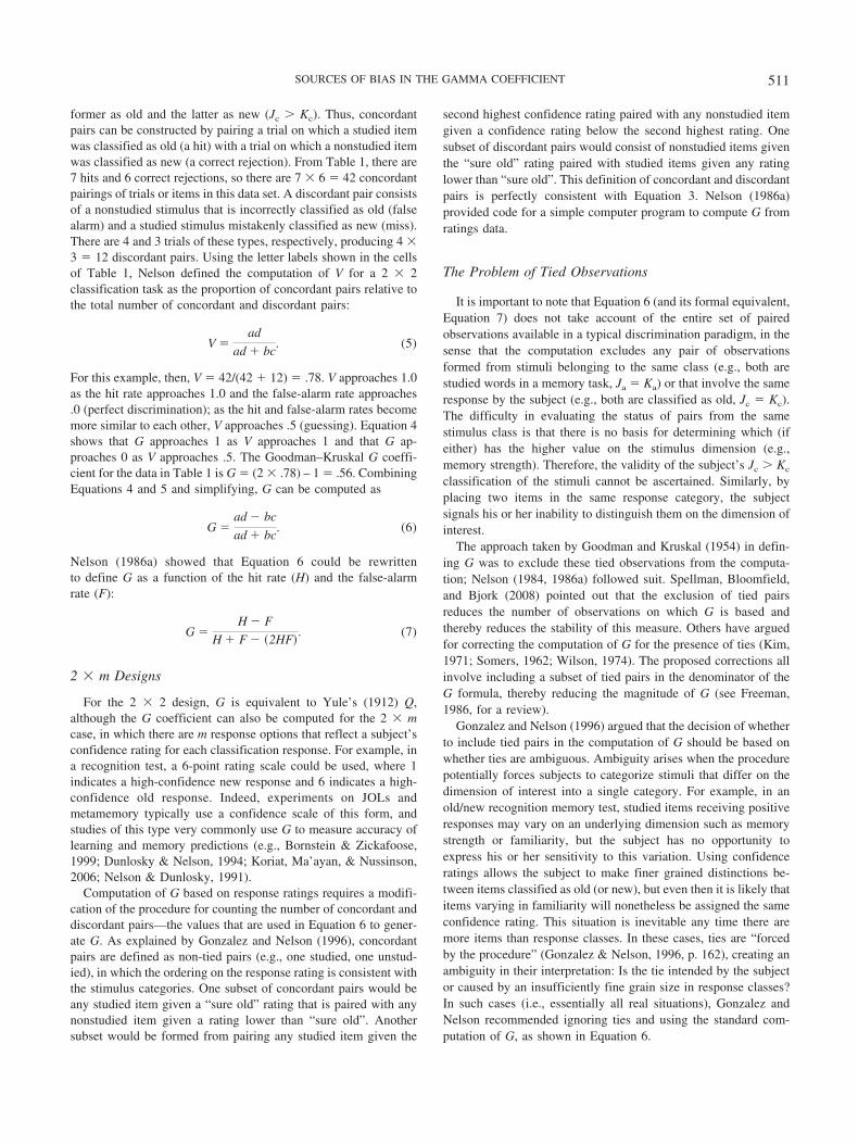
Results. The results of Simulation 1 for the equal-variancecase are presented in Figure 2, which displays, in the upper panel,the values for G calculated as in a 2 � 2 design, G based onconfidence ratings, and three versions of G corrected for ties.These observed values can be compared with the actual value of�d, shown as a horizontal line in each panel. The lower panelshows the obtained values for G� computed in the 2 � 2 case andwith confidence ratings. The associated population value for G�,shown as a horizontal line in each of the lower panels, wascomputed from the actual value of �d.
The observed values of G (uncorrected for ties) and G� consis-tently overestimated the population value, as determined by �d,and, critically, the amount of this overestimation varied acrossfalse-alarm rates. For example, at �d � .4, the observed G ex-ceeded actual �d by an amount that varied from .22 when false-alarm rate � .05 to .13 when false-alarm rate � .30. This variationin observed G is problematic because it means that even whenactual �d is constant, conditions that lead to different responsebiases, and thus different false-alarm rates, may yield spuriousdifferences in G as a measure of accuracy. The same is clearly truefor G�. Thus, it is not so much the fact that observed G and G�
deviate from the population values determined by �d but the factthat this deviation varies across false-alarm rates that is problem-atic. The correction proposed by Kim (1971) seems to vary some-what less than G across false-alarm rates, with good stability when�d � .6.
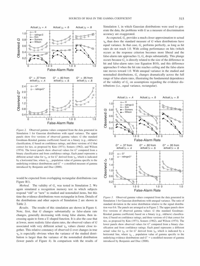
The variation in all versions of observed gamma values acrosschanges in false-alarm rate was even more pronounced when theunderlying distributions differed in variability, as the results inFigure 3 show. Under these conditions, all of the measures showeda marked decrease in magnitude as false-alarm rate increased. Forexample, the range in observed G across false-alarm rates of .05 to.50 is over .36 for an actual �d of .4. Even Kim’s (1971) correctionfares poorly under these circumstances and is worse than G when
1 We realize that this method of computing the population value of �d
may not provide the precisely correct value for �d that could be found withan analytic solution, but the simulation method is adequate for our pur-poses.
Figure 1. Flowchart showing the steps used in generating the simulationresults.
513SOURCES OF BIAS IN THE GAMMA COEFFICIENT
�d � .8. These variations in observed gamma values across false-alarm rate reflect a dramatic interaction with response bias.
Computing G and G� from confidence ratings provides for morefine-grained distinctions among items and generally reduces thenumber of observed ties. Indeed, Figures 2 and 3 reveal that G andG� based on ratings produce smaller overestimates of actual �d
than when computed from a binary classification task. Spellman etal. (2008) pointed out that, in general, a pair of items close to oneanother on the relevant stimulus dimension (e.g., similar JOLs) ismore likely than a pair that is further apart on the stimulusdimension (e.g., dissimilar JOLs) to be a discordant pair whenmemory judgments are obtained (i.e., the item given the higherJOL rating is not remembered, whereas the item given a lowerrating is remembered). With a binary classification task, however,pairs close together on the stimulus dimension are likely to beclassified together, resulting in a tied pair, which is excluded fromcalculation of G. Thus, fewer discordant pairs are generally ob-tained when computing G on the basis of a binary classificationtask rather than a ratings task. Moreover, ratings-based G varies toa smaller extent as the false-alarm rate changes. Despite thisimprovement, however, even ratings-based G systematically devi-ated from actual �d and varied as a function of false-alarm rate,particularly under conditions of unequal variance (a commonoccurrence in recognition memory studies). Thus, although usingconfidence ratings can improve the accuracy and consistency ofestimated G, systematic deviations from actual �d and variationwith response bias (false-alarm rate) continue to pose problems forthe interpretation of this measure. The same problems apply to G�.
Simulation 2: Rectangular Distributions
We have proposed that the primary source of the discrepancybetween observed G and actual �d is the loss of informationassociated with pairs of items that are tied with respect to the
subject’s responses or the stimulus categories. Moreover, we arguethat the variation in G across changing response criteria is theresult of a shift in the number of item pairs that constitute ties andin the relative numbers of those tied pairs that would have beenconcordant or discordant pairs had subjects been able to makemore fine-grained discriminations. For example, in Simulation 1,consider the case in which the standard deviation ratio is 0.6 and�d � .6 (see Figure 2). Note the substantial drop in G as thefalse-alarm rate moves from .10 to .50. That drop in G is accom-panied by a 17% increase in the number of tied pairs and a changein the ratio of concordant ties to discordant ties from 1.7 to 3.2.The larger proportion of concordant ties associated with the largerfalse-alarm rate is partly responsible for the reduction in G. Theimprovement in the behavior of G when finer grained distinctionsin responding were introduced (ratings G), thereby reducing thenumber of ties, is consistent with this proposal, although thevariability in estimated G with response bias was by no meanseliminated. Crucially, the change in the number of ties and in theratio of concordant to discordant pairs treated as ties acrosschanges in response bias will depend on the shape of the evidencedistributions from which the items are drawn.
To provide additional evidence for our claims about how tiesaffect the behavior of G, we turned to a simulation in which datawere generated from rectangular distributions. This distributionshape was chosen specifically because it afforded a straightfor-ward means of determining the proportions of tied pairs thatshould be considered as concordant or discordant. In Appendix B,we show how the computation of G should be modified to accom-plish this goal, and we develop a corrected version of G that werefer to as Gc for the special (and probably unrealistic case) ofequal-variance rectangular distributions. Computation of Gc in-cludes all observations and does not ignore ties. Rather, tied pairsare classified as concordant or discordant in proportion to what
Gaussian, �n � 0, Rectangular, �n � 0.5, Gaussian, �n � 0, n � 1, Gaussian, �f � 0, f � 1, n � 1, �s varies, n � 0.29, �s varies, �s varies, s � 1 or 1.67, �r � 1.02, r � 1.67 s � 1 or 1.67, s � 0.29 or 0.48, n/ s � 1.0 or 0.6 n/ s � 1.0 or 0.6 n/ s � 1.0 or 0.6
�d .4, .6, or .8 .4, .6, or .8 .4, .6, or .8 .4Number of items
sampled200,000 items from each
distribution200,000 items from
each distribution3 sets of 50,000 simulated
subjects; each set with 16,64, or 256 old and newitems
1,000 simulations of two groupsof 20 subjects with 64remembered and 64 forgottenitems each
Note. n � nonstudied, s � studied; for Simulation 4, f � forgotten, r � remembered. �d � population value of gamma specific to the underlying evidencedistributions; d� � signal detection measure of accuracy assuming equal-variance evidence distributions; G � the standard Goodman–Kruskal gammacoefficient; G�� a modified measure of gamma introduced by Benjamin and Diaz (2008); Gc � corrected gamma coefficient assuming rectangular evidencedistributions; da � signal detection measure of accuracy allowing for unequal-variance evidence distributions.
514 MASSON AND ROTELLO
would be expected from overlapping rectangular distributions (seeFigure B1).
Method. The validity of Gc was tested in Simulation 2. Weagain simulated a recognition memory test in which subjectsrespond “old” or “new” to studied and nonstudied items, but thistime the evidence distributions were rectangular in form. Details ofthe distributions and other aspects of Simulation 2 are shown inTable 2.
Results. The results of this simulation are shown in Figure 4.Note, first, that G changes substantially as false-alarm ratechanges, generally decreasing with rising false alarms, then in-creasing again to form a U-shaped function. It is also the case thatat lower, more realistic false-alarm rates, the observed values of Gassociated with very different actual �d values cluster close to-gether. This relative constancy of observed G over changes in true�d is especially obvious when the variance of the studied distri-bution is larger than the variance of the nonstudied distribution(lower panels of Figure 4). In comparison with the results of
Simulation 1, in which Gaussian distributions were used to gen-erate the data, the problems with G as a measure of discriminationaccuracy are exaggerated.
As expected, Gc provides a much closer approximation to actual�d than does the standard measure of G when distributions haveequal variance. In that case, Gc performs perfectly, as long as hitrates do not reach 1.0. With ceiling performance on hits (whichoccurs as the response criterion becomes more liberal and thefalse-alarm rate approaches 1), Gc drops substantially. This plungeoccurs because Gc is directly related to the size of the difference inhit and false-alarm rates (see Equation B10), and this differenceapproaches 0 when the hit rate reaches ceiling and the false-alarmrate moves toward 1.0. With unequal variance in the studied andnonstudied distributions, Gc changes dramatically across the fullrange of false-alarm rates, illustrating the fundamental dependenceof the validity of Gc on assumptions regarding the evidence dis-tributions (i.e., equal variance, rectangular).
Actual = .4
False-Alarm Rate0 1.0
ratings GG
KimSomersWilson
Actual = .6 Actual = .8
G* = .37 from actual = .4
0 1.0 0 1.0
0.4
0.8
1.2
1.6
2.0
2.4 G*ratings G*
0.2
0.4
0.6
0.8
1.0
False-Alarm Rate0 1.0 0 1.0 0 1.0
G* = .60 from actual = .6
G* = .95 from actual = .8γd
γdγdγd
γd γd
Figure 2. Observed gamma values computed from the data generated inSimulation 1 for Gaussian distributions with equal variance. The upperpanels show five versions of observed gamma values: G (the standardGoodman–Kruskal gamma coefficient) based on a binary (e.g., old/new)classification, G based on confidence ratings, and three versions of G thatcorrect for ties, as proposed by Kim (1971); Somers (1962), and Wilson(1974). The lower panels show observed values for G� computed from abinary classification and from confidence ratings. Each panel represents adifferent actual value for �d, or for G� derived from �d, which is indicatedby a horizontal line, where �d � population value of gamma specific to theunderlying evidence distributions and G� � a modified measure of gammaintroduced by Benjamin and Diaz (2008).
Actual = .4
False-Alarm Rate
ratings GG
KimSomersWilson
Actual = .6 Actual = .8
0 1.0 0 1.0
G*ratings G*
0.2
0.4
0.6
0.8
1.0
False-Alarm Rate0 1.0 0 1.0 0 1.0
0 1.0
0.2
0.6
1.0
1.4
1.8
2.2
G* = .37 from actual = .4
G* = .60 from actual = .6
G* = .95 from actual = .8
γd γd γd
γdγdγd
Figure 3. Observed gamma values computed from the data generated inSimulation 1 for Gaussian distributions with unequal variance. The ratio ofstandard deviation in the noise distribution relative to the signal distribu-tion was 0.6. The panels are arranged as in Figure 2. The upper panels showfive versions of observed gamma values: G (the standard Goodman–Kruskal gamma coefficient) based on a binary (e.g., old/new) classifica-tion, G based on confidence ratings, and three versions of G that correct forties, as proposed by Kim (1971), Somers (1962), and Wilson (1974). Thelower panels show observed values for G� computed from a binary clas-sification and from confidence ratings. Each panel represents a differentactual value for �d, or for G� derived from �d, which is indicated by ahorizontal line, where �d � population value of gamma specific to theunderlying evidence distributions and G� � a modified measure of gammaintroduced by Benjamin and Diaz (2008).
515SOURCES OF BIAS IN THE GAMMA COEFFICIENT
The results of Simulation 2 confirm our claim that the bias in Gthat we have demonstrated is due to the fact that the computationof G ignores tied pairs of observations. When correct proportionsof these ties can be defined as concordant versus discordant pairs,G can be computed with perfect accuracy. This computation,however, requires specific information about the shape of thedistributions from which observations are drawn, particularly inthe regions occupied by tied observations, and about the relativevariance of the distributions. To reinforce this point, we computedGc for the data generated in Simulation 1. The results are shown inFigure 5. When applied to data generated by Gaussian distribu-tions, the estimated values of Gc show substantial variation acrosschanges in the false-alarm rate while �d is held constant. As withthe simulation of data from rectangular distributions, the large fallin Gc as the false-alarm rate approaches 1 in the equal-variancecase (upper panel of Figure 4) is due to H hitting ceiling. Unlikethe situation with rectangular distributions, however, Gc changessubstantially across lower values of the false-alarm rate even whenthe distributions have equal variance. It is clear that Gc is usefulonly when the specific distributional assumptions underlying itsderivation hold. We do not, therefore, advocate Gc as a replace-
ment for G, and we suspect that it would be rare for distributionsunderlying actual data to conform to rectangular shape. Our intro-duction of Gc here was specifically intended to demonstrate thereason for the variation in observed values of G as responsecriterion changes.
Simulation 3: Population �d and Estimation Accuracy
We have identified two problems with G computed from sampledata when it is used as an estimate of discrimination accuracy.First, G systematically deviates from the true population value of�d, even when a correction for tied observations is included in thecomputation of G. Second, G varies, sometimes substantially, as afunction of response bias even though the population value �d isconstant across these changes. Although the concern regardingresponse bias is demonstrated here for the first time, the traditionalstatistics literature previously has addressed the properties of G asan estimator of �, defined in the classical manner.
In the statistics literature, interest has centered on the accuracywith which sample-based G estimates �. Goodman and Kruskal(1963, 1972) demonstrated that with asymptotically large samples,
Actual = .4
False-Alarm Rate
GcG
Actual = .6 Actual = .8
0 1.0 0 1.0
0.2
0.4
0.6
0.8
1.0
False-Alarm Rate0 1.0 0 1.0 0 1.0
0 1.0
Actual = .4 Actual = .6 Actual = .8
0.2
0.4
0.6
0.8
1.0
γd γd γd
γd γdγd
Figure 4. Observed G (the standard Goodman–Kruskal gamma coeffi-cient) values computed from the data generated in Simulation 2 for rect-angular distributions using Equation 6 and the corrected version of Gderived in Appendix B, Gc. The upper panels show the equal-variance case,and the lower panels present the data for unequal-variance distributions,where the ratio of noise to signal distribution standard deviations is 0.6.Each panel represents a different actual value for �d (population value ofgamma specific to the underlying evidence distributions), which is indi-cated by a horizontal line. .2
.4
.6
.8
1.0
0.0 1.0
False-Alarm Rate
.2
.4
.6
.8
1.0
.4.6.8
Actualγd
Figure 5. Observed Gc (corrected gamma coefficient assuming rectan-gular evidence distributions) values computed from the data generated inSimulation 1 for Gaussian distributions. The upper panel presents resultsfor the equal-variance case, and the lower panel displays results for anoise/signal standard deviation ratio of 0.6. Each symbol type shows thevalue of Gc computed when a different actual value of �d (population valueof gamma specific to the underlying evidence distributions) was in effect.Actual values of �d are also indicated by the horizontal lines in each panel.
516 MASSON AND ROTELLO
G is an unbiased estimate of �. For small to moderate sample sizesand the 2 � 2 and 2 � 3 cases, however, the distribution of sampleG values has rather high variability and is irregular and skewed,resulting in a biased estimate of �. Moreover, the distribution of Gconverges very slowly to the ideal form reported by Goodman andKruskal for the asymptotic case (Gans & Robertson, 1981a, 1981b;see also Lui & Cumberland, 2004; Rosenthal, 1966; Woods,2007).
Method. In Simulation 3, we examined bias and variability inobserved values of G relative to �d by simulating data for a largenumber of subjects, each of whom contributes a G value deter-mined by a defined number of observations, as is done in thestatistical literature when assessing the convergence of observed Gto actual �. We also included G� (Benjamin & Diaz, 2008) in thesesimulations to compare its convergence properties to those of G.Details of this simulation are shown in Table 2. The numbers oftrials on which each simulated subject’s data were based matchedthe numbers used by Verde, Macmillan, and Rotello (2006) in theirinvestigation of alternative measures of discrimination accuracy,thereby allowing us to compare our results with those they re-ported.
For simulation of the old/new task, we computed G and G� foreach subject but excluded any subjects for whom these measureswere undefined (e.g., G is undefined if H � F � 0; G� is undefinedif G � 1.0). To reduce the number of observations lost due toextreme outcomes, following Verde et al. (2006), we also com-puted G and G� based on a log-linear transformation of hit andfalse alarm rates, such that H � (Th � 0.5)/(T � 1) and F � (Tf �0.5)/(T � 1), where Th and Tf are the number of hits and falsealarms, respectively, and T is the number of signal trials and thenumber of noise trials. Loss of observations due to extreme out-comes was not a problem in Simulations 1 and 2 because in thosecases, we were not simulating individual subjects whose data werebased on relatively few observations. Rather, those simulationswere based on tens of thousands of trials for each computation ofa measure, so ceiling or floor values (1 and 0) were never encoun-tered.
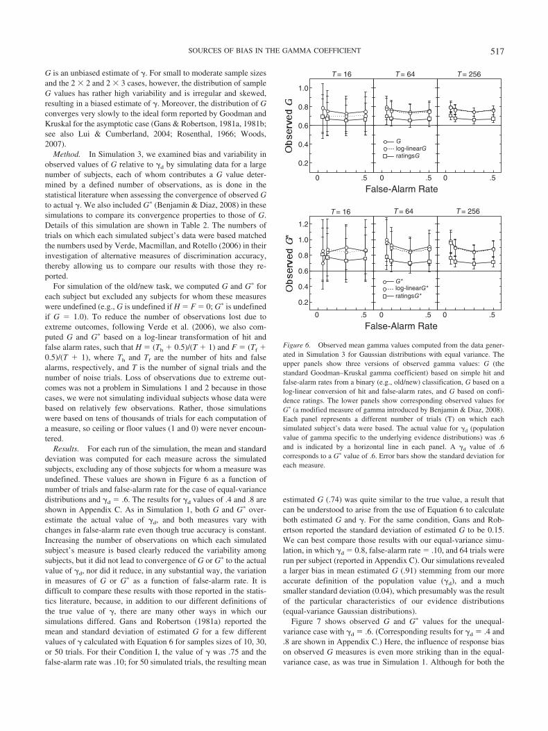
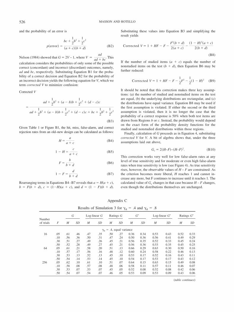
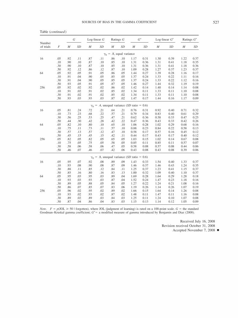
Results. For each run of the simulation, the mean and standarddeviation was computed for each measure across the simulatedsubjects, excluding any of those subjects for whom a measure wasundefined. These values are shown in Figure 6 as a function ofnumber of trials and false-alarm rate for the case of equal-variancedistributions and �d � .6. The results for �d values of .4 and .8 areshown in Appendix C. As in Simulation 1, both G and G� over-estimate the actual value of �d, and both measures vary withchanges in false-alarm rate even though true accuracy is constant.Increasing the number of observations on which each simulatedsubject’s measure is based clearly reduced the variability amongsubjects, but it did not lead to convergence of G or G� to the actualvalue of �d, nor did it reduce, in any substantial way, the variationin measures of G or G� as a function of false-alarm rate. It isdifficult to compare these results with those reported in the statis-tics literature, because, in addition to our different definitions ofthe true value of �, there are many other ways in which oursimulations differed. Gans and Robertson (1981a) reported themean and standard deviation of estimated G for a few differentvalues of � calculated with Equation 6 for samples sizes of 10, 30,or 50 trials. For their Condition I, the value of � was .75 and thefalse-alarm rate was .10; for 50 simulated trials, the resulting mean
estimated G (.74) was quite similar to the true value, a result thatcan be understood to arise from the use of Equation 6 to calculateboth estimated G and �. For the same condition, Gans and Rob-ertson reported the standard deviation of estimated G to be 0.15.We can best compare those results with our equal-variance simu-lation, in which �d � 0.8, false-alarm rate � .10, and 64 trials wererun per subject (reported in Appendix C). Our simulations revealeda larger bias in mean estimated G (.91) stemming from our moreaccurate definition of the population value (�d), and a muchsmaller standard deviation (0.04), which presumably was the resultof the particular characteristics of our evidence distributions(equal-variance Gaussian distributions).
Figure 7 shows observed G and G� values for the unequal-variance case with �d � .6. (Corresponding results for �d � .4 and.8 are shown in Appendix C.) Here, the influence of response biason observed G measures is even more striking than in the equal-variance case, as was true in Simulation 1. Although for both the
0.2
0.4
0.6
0.8
1.0
Glog-linear Gratings G
0.2
0.4
0.6
0.8
1.0
1.2
G*log-linear G*ratings G*
T = 16 T= 64 T= 256
T = 16 T = 64 T = 256
0 .5
False-Alarm Rate0 .5 0 .5
0 .5
False-Alarm Rate0 .5 0 .5
Figure 6. Observed mean gamma values computed from the data gener-ated in Simulation 3 for Gaussian distributions with equal variance. Theupper panels show three versions of observed gamma values: G (thestandard Goodman–Kruskal gamma coefficient) based on simple hit andfalse-alarm rates from a binary (e.g., old/new) classification, G based on alog-linear conversion of hit and false-alarm rates, and G based on confi-dence ratings. The lower panels show corresponding observed values forG� (a modified measure of gamma introduced by Benjamin & Diaz, 2008).Each panel represents a different number of trials (T) on which eachsimulated subject’s data were based. The actual value for �d (populationvalue of gamma specific to the underlying evidence distributions) was .6and is indicated by a horizontal line in each panel. A �d value of .6corresponds to a G� value of .6. Error bars show the standard deviation foreach measure.
517SOURCES OF BIAS IN THE GAMMA COEFFICIENT
equal- and the unequal-variance cases, the G estimates seem toconverge toward the true value of �d as the false-alarm rateincreases, Simulation 1 shows that this is a deceiving trend in thatG estimates increase sharply once false-alarm rate exceeds .5 in theequal-variance case (see Figure 2), and they decrease markedly inthe unequal-variance case, leading to underestimates of �d (seeFigure 3).
Comparable simulations reported by Verde et al. (2006) usingthe signal detection measure Az, which is closely related to the da
measure presented earlier in the introduction (see Appendix A),show that Az has much smaller variability than does G. Forexample, across a range of false-alarm rates, with actual accuracysimilar to �d � .6, and equal-variance Gaussian distributions,Verde et al. obtained standard deviations of the Az estimate rangingfrom approximately .08 to .02 for sample sizes that varied from 16to 256. In our simulations with G, the corresponding standard
deviations ranged from approximately .20 to .05 (ratings G wasonly slightly better and log-linear G was worse). The samplingvariability for G� was even larger than that for G, in part becauseG� takes on a wider range of possible values. Thus, Simulation 3,in conjunction with the Verde et al. simulations, shows that sam-pling variability for G is generally larger than for Az, a measurebased on signal detection theory.
A Signal Detection Alternative to G
Desirable properties of an accuracy measure are independencefrom response bias, low statistical bias, and a low standard error.Our first three simulations showed that G and ratings G fail on allcounts. In addition, a successful measure must be consistent withthe observed form of the empirical receiver operating characteris-tic (ROC). Swets (1986a) showed that, for a range of disciplines,empirical ROCs are consistent with underlying evidence distribu-tions that are approximately Gaussian in form and unequal invariance (like the recognition ROCs in Figure 8 and themetamemory ROCs in Figure 9). Here, too, G fails because it ismost consistent with equal-variance logistic distributions (Swets,1986b). Requiring an accuracy measure to be consistent withunequal-variance Gaussian distributions eliminates a number ofcommonly used measures, including percentage or proportion cor-rect, recognition scores corrected for bias (i.e., Pr � hit rate –false-alarm rate), and A� (Verde et al., 2006; Rotello, Masson, &Verde, 2008). Even d� fails these tests, as it does not always havelow statistical bias or a low standard error (Miller, 1996), and it isindependent of response bias only when the data are drawn fromequal-variance Gaussian distributions (Macmillan & Creelman,2005; Rotello et al., 2008).
In contrast, the accuracy measure Az, which estimates the areaunder the ROC for data drawn from any distributions that can bemonotonically transformed to equal- or unequal-variance Gaussiandistributions, satisfies all of our criteria: It has very low statisticalbias, has a low standard error, and is not affected by the standarddeviation ratio of the underlying distributions (Macmillan, Rotello,& Miller, 2004; Verde et al., 2006). Indeed, Swets (1986a) arguedthat the consistency of the form of the empirical ROCs acrossfields “supports the use of the accuracy index Az” (p. 196). Thevariable da is a distance-based measure that shares the desirableproperties of Az, including independence from response bias (seeMacmillan et al., 2004; Rotello et al., 2008), and is monotonicallyrelated to it (see Equation A1). Thus, use of either Az or da is welljustified.
Simulation 4: A Simulated Metacognitive Experiment
In Simulation 4, we demonstrate that with realistic numbers ofobservations and subjects, G and ratings G are likely to produceartifactual indications of accuracy differences between conditionsthat vary only with respect to response bias. Moreover, we dem-onstrate that the signal detection–based measure da avoids thisproblem. We base our simulation on the observation that a numberof experiments on metamemory have shown that the estimates ofthe FOK or JOLs are influenced by factors such as the delaybetween study exposure and the metamemory decision on eachitem. G (or ratings G) is smaller when a JOL for an item is madeat the same time that the item is studied, relative to when JOLs are
0.2
0.4
0.6
0.8
1.0
1.2
1.4
0.2
0.4
0.6
0.8
1.0
Glog-linear Gratings G
G*log-linear G*ratings G*
T = 16 T= 64 T = 256
T = 16 T = 64 T = 256
0 .5
False-Alarm Rate0 .5 0 .5
0 .5
False-Alarm Rate0 .5 0 .5
Figure 7. Observed mean gamma values computed from the data gener-ated in Simulation 3 for Gaussian distributions with unequal variance. Theratio of standard deviation in the noise distribution relative to the signaldistribution was 0.6. The panels are arranged as in Figure 6: The upperpanels show three versions of observed gamma values: G (the standardGoodman–Kruskal gamma coefficient) based on simple hit and false-alarmrates from a binary (e.g., old/new) classification, G based on a log-linearconversion of hit and false-alarm rates, and G based on confidence ratings.The lower panels show corresponding observed values for G� (a modifiedmeasure of gamma introduced by Benjamin & Diaz, 2008). Each panelrepresents a different number of trials (T) on which each simulated sub-ject’s data were based. The actual value for �d (population value of gammaspecific to the underlying evidence distributions) was .6 and is indicated bya horizontal line in each panel. A �d value of .6 corresponds to a G� valueof .6. Error bars show the standard deviation for each measure.
518 MASSON AND ROTELLO
collected after even a brief delay (for a review, see Schwartz,1994). Subject-related factors have also been shown to influence Gin theoretically interesting ways. For example, Souchay, Moulin,Clarys, Taconnat, and Isingrini (2007) reported that older adults’FOK judgments on episodic memory tasks were less accurate thanthose of younger adults’: Ratings G was lower for the oldersubjects. The authors’ interpretation was that older adults are lessable to use a recollective memory process that is essential foraccurate episodic FOK judgments. Another explanation of this agedifference in ratings G is that it is the result of a response biaseffect. That is, the older adults in Souchay et al.’s Experiment 2used a more liberal response criterion than did the younger adults(false-alarm rate � 0.22 for older adults and 0.16 for youngeradults).2 The results of our Simulation 1 (Figures 2 and 3) showedthat both G and ratings G decrease as the response criterionbecomes more liberal (at least over the range of false alarms
exhibited by the two age groups in the Souchay et al. study). It isreasonable to ask, then, whether the difference in the observedgamma correlations is a real effect based in a memory ormetamemory process or an effect that is driven by the differentresponse criteria used by the younger and older subjects. Givenonly the data reported by Souchay et al., we cannot definitivelyseparate accuracy effects from response bias effects.
In this section, we simulate the consequences of a response-biasdifference across conditions in a metacognitive experiment. Theresulting data are reported for G, ratings G, and two signal-detection based statistics, d� and da. Other measures related to Gthat we examined in earlier simulations, such as G�, show the samepattern of behavior as G, both in Simulation 4 and in our evalua-tion of actual empirical data presented below. The advantage ofusing a simulation is that we know the two simulated conditionshave a common level of true accuracy but different responsebiases. Thus, we can evaluate the probability that significance testswith each accuracy measure would lead the researcher to theincorrect conclusion that the two conditions differ in accuracy(e.g., that G differs reliably between groups). In other words,Simulation 4 estimates the Type I error rate for each measureunder conditions of changing response bias (see also Rotello et al.,2008). In the next section, we consider how these same accuracymeasures fare with actual empirical data from two publishedexperiments.
Method. In Simulation 4, we assumed that there are two ex-perimental conditions in which each subject has the same trueaccuracy level of �d � 0.4 but that subject in the conservativecondition have an average false-alarm rate that is lower than thatof subjects in the liberal condition. Details of the evidence distri-
2 Most metamemory experiments use recall or cued recall to assessmemory performance. Of those that use recognition, most report only theoverall percentage of correct memory judgments, from which response biascannot be determined. Of course, the absence of information about re-sponse bias does not eliminate the problems created by differences inresponse bias.
12345
.0
.2
.4
.6
.8
1.0Recall Task
.0 .2 .4 .6 .8 1.0
p (JOL | Forgotten)
Recognition Task
.0 .2 .4 .6 .8 1.0
p (JOL | Forgotten)
.0
.2
.4
.6
.8
1.0
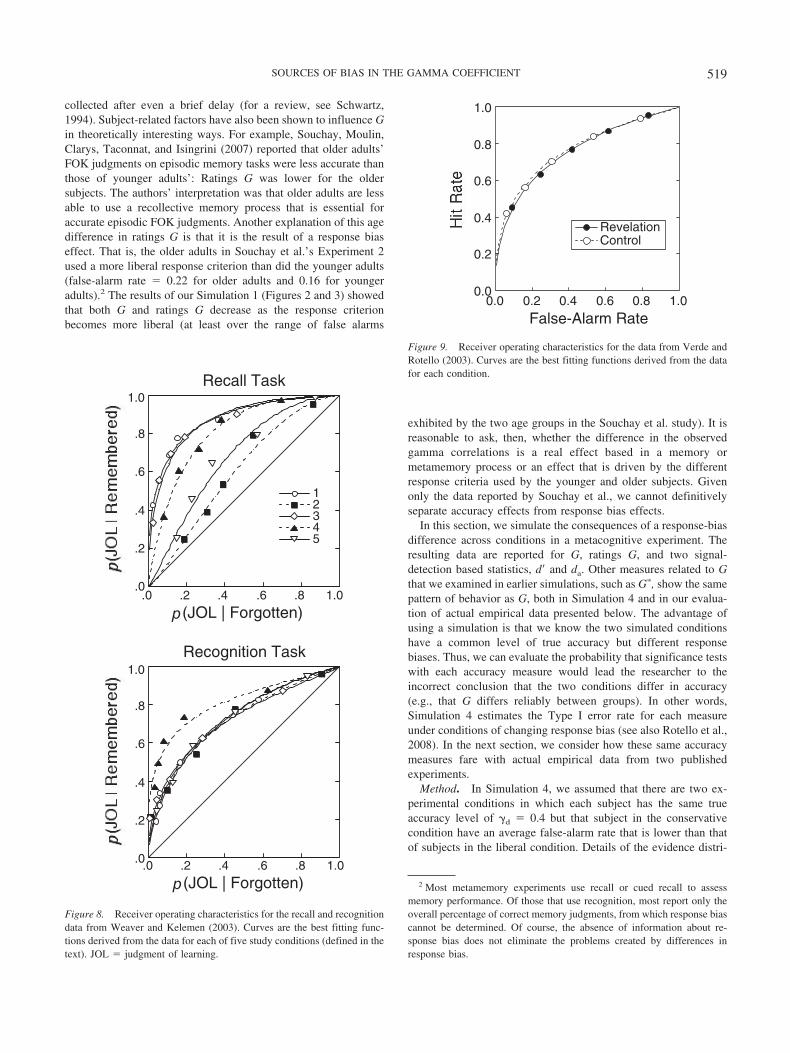
Figure 8. Receiver operating characteristics for the recall and recognitiondata from Weaver and Kelemen (2003). Curves are the best fitting func-tions derived from the data for each of five study conditions (defined in thetext). JOL � judgment of learning.
0.0
0.2
0.4
0.6
0.8
1.0
0.0 0.2 0.4 0.6 0.8 1.0
False-Alarm Rate
RevelationControl
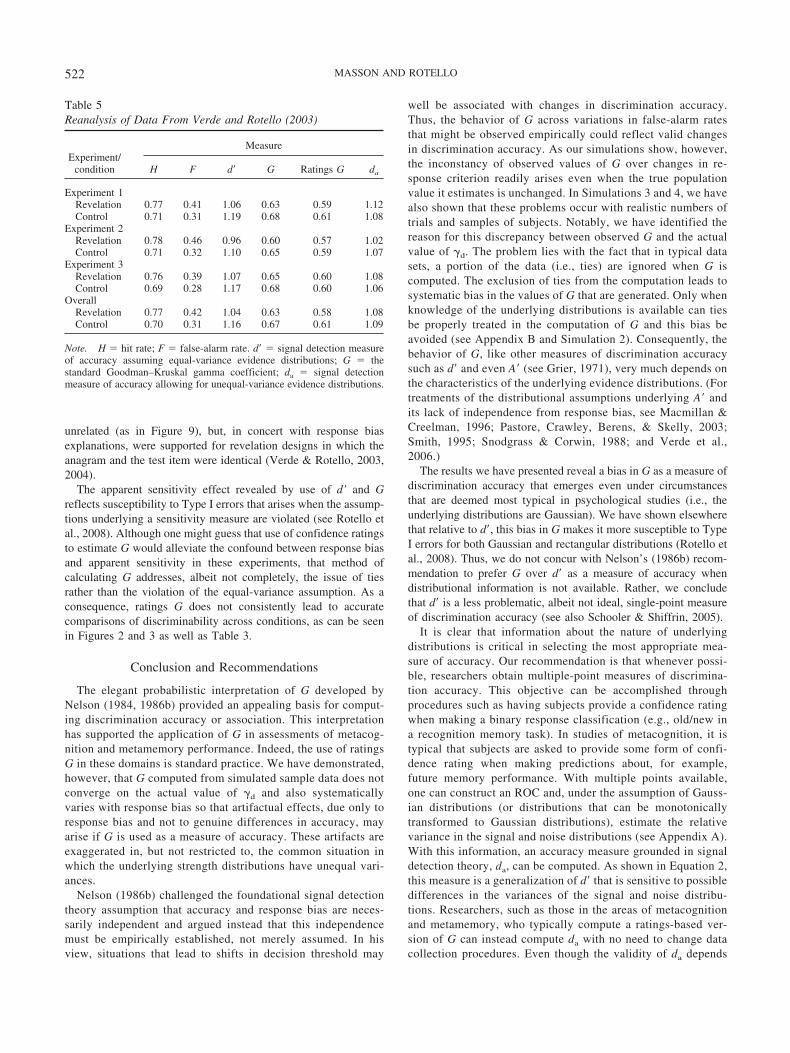
Figure 9. Receiver operating characteristics for the data from Verde andRotello (2003). Curves are the best fitting functions derived from the datafor each condition.
519SOURCES OF BIAS IN THE GAMMA COEFFICIENT
butions and other aspects of the simulation are shown in Table 2.Note that in this simulation, larger variance was assumed for thedistribution of remembered items than for the distribution offorgotten items.
Results. If G and ratings G were unbiased estimators of true�d, then both would have average values of around 0.4. Table 3shows that both measures overestimate the true value, and theamount of overestimation is larger in the conservative condition. Inaddition, all of the 1,000 t tests (one per simulated experiment)declared that the two conditions differed significantly, both on Gand on ratings G. In other words, the Type I error rate for thesemeasures was 1.0. Similar results were reported by Rotello et al.(2008) for a wide range of simulated experimental conditions.
Use of the signal detection measure d� to assess memory accu-racy in this simulation also led to a Type I error rate of 1.0 (seeTable 3 and Rotello et al., 2008) because d� is confounded withresponse bias when the underlying distributions are of unequalvariance (Macmillan & Creelman, 2005). In contrast, the da mea-sure, which generalizes d� to the unequal-variance situation (seeEquation 2), yielded a Type I error rate near the standard alphalevel of 5%. Moreover, the mean da value in each condition is 0.75,which is essentially identical to the theoretical value of 0.74 forthese distributions.
The implications of Simulation 4, as well as the related simu-lations reported by Rotello et al. (2008), are quite broad. Use of G,ratings G, or d� to measure metacognitive performance may mis-lead researchers about the nature of the differences between con-ditions. When the underlying metamemory or memory distribu-tions have unequal variance and only response bias differs betweenconditions, all of these measures misattribute those bias differ-ences to accuracy effects. Only da provides an appropriate descrip-tion of metamemory accuracy.
Two Numerical Examples With Real Data
Using simulations, we have demonstrated that G is associatedwith four disadvantages relative to accuracy measures based onsignal detection: (a) It is modulated by varying response criteriaeven when actual accuracy is constant; (b) it does not asymptoti-cally converge on the true value of �d; (c) its sampling variabilityis large; and (d) it yields an unacceptably high Type I error ratewhen accuracy is constant across conditions but response biasdiffers. We now consider how G and ratings G, as well as thesignal-detection–based measures d� and da, fare in two real datasets. For our evaluations, we chose examples in which confidence
ratings were collected so that the form of the underlying evidencedistributions, and therefore true sensitivity, could be estimatedaccurately. The availability of confidence ratings also allows com-putation of both ratings G and da. We selected one example fromthe metamemory literature (Weaver & Kelemen, 2003) in which Gis used most heavily and a second example from the recognitionmemory literature where d� dominates (Verde & Rotello, 2003).
Metamemory example. Weaver and Kelemen (2003) askedsubjects to make JOLs on cue–target word pairs (e.g.,ELEPHANT–sunburn) and later to recall the target word in re-sponse to the cue or to recognize the correct cue–target pair froma set that included 6 lure pairs. The theoretical motivation for theauthors’ study was to test whether the accuracy of the JOLsreflected transfer-appropriate monitoring. That is, if the JOLs weregenerated under conditions that more closely mimicked the testconditions, would they be more accurate? To find out, Weaver andKelemen collected the JOLs in five conditions. In Condition 1, theJOL probe consisted of only the cue word (ELEPHANT–?) fromeach pair. This condition mimicked a cued recall task. In Condition2, the JOL probe consisted of the cue–target pair (ELEPHANT–sunburn). In Condition 3, the JOL probe was the cue word(ELEPHANT–?), but it was shown in the context of 6 lure pairs(ELEPHANT– diamond, ELEPHANT– hillside, ELEPHANT–sugar, etc.); this condition reflected a mixture of cued-recall andrecognition tasks. Condition 4 was similar to Condition 3, exceptthat the entire cue–target pair (ELEPHANT–sunburn) was pre-sented with the lures; this condition mimicked the recognition task.Finally, Condition 5 was identical to Condition 4 except that thecorrect cue–target pair was marked (ELEPHANT–sunburn���).
Weaver and Kelemen (2003) reported ratings G correlations ofthe JOLs in each condition with the eventual memory perfor-mance, predicting that Condition 1 would show the highest ratingsG when computed using cued recall data and that Condition 4would show the highest ratings G when computed using recogni-tion data. The results, shown in the ratings G column of Table 4,do not support the transfer-appropriate monitoring hypothesis.Ratings G was higher in Condition 1 than in Conditions 2 or 5when recall data were used, but it was equal to that in Conditions3 and 4. When the recognition data were used, Condition 4’sratings G was among the lowest of all. For these reasons, Weaverand Kelemen rejected transfer-appropriate monitoring as a possi-ble theoretical account of metamemory judgments, concluding thatalternative theories better accounted for their results.
Table 3Results of Simulation 4: A Simulated Metacognition Experiment in Which Conditions Differ Only in Response Bias
Note. Values for d’ are based on log-linear corrections for 0s and 1s in the hit and false-alarm rates of individual simulated subjects. H � p(FOK �50 | remembered); F � p(FOK � 50 | forgotten), where FOK (feeling of knowing) is rated on a 100-point scale. d� � signal detection measure of accuracyassuming equal-variance evidence distributions; G � the standard Goodman–Kruskal gamma coefficient; da � signal detection measure of accuracyallowing for unequal-variance evidence distributions.
520 MASSON AND ROTELLO
We used the JOL ratings to create metamemory ROCs, employ-ing a method that Benjamin and Diaz (2008) described in detail(see also Nelson, 1984). Analogous to the recognition ROCs,metamemory ROCs plot accurate responses (remembered items)on the y-axis and errors (forgotten items) on the x-axis as afunction of JOL rating. Thus, the first point on each ROC reflectsmetamemory accuracy for items that subjects were sure theywould remember (JOL � 100%), the second point indicates re-sponses to items that subjects were quite confident about (JOL �80%), and so forth. The resulting metamemory ROCs are shown inFigure 8; curves higher in the space reflect greater metamemoryaccuracy. There are two striking effects. First, Conditions 1 and 3fall higher than the others when the recall data are considered;second, Condition 4 falls well above the others when recognitiondata are used. Weaver and Kelemen predicted this pattern ofmetamemory accuracies on the principle of transfer-appropriateprocessing but did not observe it with ratings G.
We computed d�, da, and nonrating G for these data, assumingthat a hit was a remembered item to which subjects had assigneda JOL of at least 50%, and a false alarm was a forgotten item givena similar JOL. Thus, H � p(JOL � 50 | remembered) and F �p(JOL � 50 | forgotten). Because the metamemory ROCs inFigure 8 are roughly consistent with underlying distributions thatare unequal-variance Gaussian in form, and because response biasdifferences are evident across conditions, we expected that da
would provide the best description of metamemory accuracy, as itdid in Simulation 4. In other words, we expected da to show apattern consistent with the varying heights of the metamemoryROCs across JOL conditions. The resulting values, shown in Table4, are consistent with that expectation.3 The implication of thisanalysis is startling. Had Weaver and Kelemen used da rather thanratings G to assess metamemory accuracy, they would havereached the opposite theoretical conclusion, finding support fortheir preferred theory (transfer-appropriate monitoring) andagainst the alternatives.
Recognition memory example. Verde and Rotello (2003) col-lected confidence ratings in three within-subject recognition mem-ory experiments. In each experiment, subjects studied a list ofwords and then were given a recognition test that consisted of bothstudied and nonstudied items. In the revelation conditions, subjectswere asked to solve an anagram immediately prior to making theirrecognition judgment for a particular item (the anagram and testword were unrelated); in the control conditions, there were noanagrams. The substantive question of interest was whether mem-ory sensitivity was affected by the revelation task. In each exper-iment, the hit and false-alarm rates were both higher in the reve-lation condition than in the control condition (see Table 5). Theseresponse rates can be used to compute single-point sensitivitystatistics. In the literature on the revelation effect, d’ is used mostcommonly. Its application suggests that accuracy is decreased bythe revelation task, significantly so when considered across exper-iments, t(81) � 2.09, p � .05. Application of G supports thatconclusion, t(81) � 1.71, p � .09, but use of ratings G reduces thedifference to a nonsignificant level, t(81) � 1.06, p � .25. On thebasis of d’ results like these, the revelation effect previously hadbeen attributed to an increase in the familiarity of the test itemsduring the revelation task (see Hicks & Marsh, 1998, for a meta-analysis).
In this case, however, only ratings G accurately describes theeffect of the revelation task on memory accuracy. Verde andRotello (2003) used the confidence rating data to estimate thestandard deviation ratios of the distributions underlying the non-studied and studied items, which was about 0.8. When the standarddeviation ratio is less than 1, larger values of d� are estimated formore conservative response criteria that result in lower hit andfalse-alarm rates (i.e., the control conditions). Analogous problemsexist for G (and ratings G; see Figures 2 and 3 and Table 3), whichis consistent with equal-variance logistic distributions (see Swets,1986b). Verde and Rotello computed the more appropriate statisticda and found no sensitivity differences across conditions, t(81) �0.06. Consistent with this conclusion, we show in Figure 9 theROCs for the revelation and control conditions on the basis ofconfidence-rating data aggregated across the three experiments(these data are available in the Appendix of the Verde & Rotelloarticle). Note that the two curves in Figure 9 fall at a nearlyidentical height in the space, indicating very similar levels ofdiscrimination accuracy. Use of the more appropriate statistic da
provided theoretical insight on the revelation literature:Familiarity-based explanations of the effect were eliminated forrevelation designs in which the anagram and the test item were
3 Bill Kelemen very kindly provided the data from this experiment, butthe ROCs were extremely unstable at the individual subject level becausethere were too few trials per condition. Therefore, statistical comparison ofthese measures across JOL conditions was not possible, and we based ourestimates of G and the signal detection measures on the group data. Theindividual data do allow clarity on one curious aspect of these data, whichis that ratings G does not appear to capture the pattern of performance aswell as G. A number of subjects achieved perfect recall or recognition inone condition or another, and G cannot be computed from data of this formbecause all items pairs are ties (see the program in Nelson, 1986a). Thus,these subjects were omitted from the analyses reported by Weaver andKelemen (2003). When ratings G is calculated on the group data, however,the resulting values mimic the order of the ROCs in Figure 8.
Table 4Reanalysis of Data From Weaver and Kelemen (2003)
Note. JOL (judgment of learning) conditions marked with an asteriskwere predicted by Weaver and Kelemen (2003) to produce the best meta-cognitive performance. H � p(JOL � 50 | remembered); F � p(JOL �50 | forgotten), where JOL is rated on a 100-point scale. d� � signal detectionmeasure of accuracy assuming equal-variance evidence distributions; G � thestandard Goodman–Kruskal gamma coefficient; da � signal detection measureof accuracy allowing for unequal-variance evidence distributions.
521SOURCES OF BIAS IN THE GAMMA COEFFICIENT
unrelated (as in Figure 9), but, in concert with response biasexplanations, were supported for revelation designs in which theanagram and the test item were identical (Verde & Rotello, 2003,2004).
The apparent sensitivity effect revealed by use of d’ and Greflects susceptibility to Type I errors that arises when the assump-tions underlying a sensitivity measure are violated (see Rotello etal., 2008). Although one might guess that use of confidence ratingsto estimate G would alleviate the confound between response biasand apparent sensitivity in these experiments, that method ofcalculating G addresses, albeit not completely, the issue of tiesrather than the violation of the equal-variance assumption. As aconsequence, ratings G does not consistently lead to accuratecomparisons of discriminability across conditions, as can be seenin Figures 2 and 3 as well as Table 3.
Conclusion and Recommendations
The elegant probabilistic interpretation of G developed byNelson (1984, 1986b) provided an appealing basis for comput-ing discrimination accuracy or association. This interpretationhas supported the application of G in assessments of metacog-nition and metamemory performance. Indeed, the use of ratingsG in these domains is standard practice. We have demonstrated,however, that G computed from simulated sample data does notconverge on the actual value of �d and also systematicallyvaries with response bias so that artifactual effects, due only toresponse bias and not to genuine differences in accuracy, mayarise if G is used as a measure of accuracy. These artifacts areexaggerated in, but not restricted to, the common situation inwhich the underlying strength distributions have unequal vari-ances.
Nelson (1986b) challenged the foundational signal detectiontheory assumption that accuracy and response bias are neces-sarily independent and argued instead that this independencemust be empirically established, not merely assumed. In hisview, situations that lead to shifts in decision threshold may
well be associated with changes in discrimination accuracy.Thus, the behavior of G across variations in false-alarm ratesthat might be observed empirically could reflect valid changesin discrimination accuracy. As our simulations show, however,the inconstancy of observed values of G over changes in re-sponse criterion readily arises even when the true populationvalue it estimates is unchanged. In Simulations 3 and 4, we havealso shown that these problems occur with realistic numbers oftrials and samples of subjects. Notably, we have identified thereason for this discrepancy between observed G and the actualvalue of �d. The problem lies with the fact that in typical datasets, a portion of the data (i.e., ties) are ignored when G iscomputed. The exclusion of ties from the computation leads tosystematic bias in the values of G that are generated. Only whenknowledge of the underlying distributions is available can tiesbe properly treated in the computation of G and this bias beavoided (see Appendix B and Simulation 2). Consequently, thebehavior of G, like other measures of discrimination accuracysuch as d� and even A� (see Grier, 1971), very much depends onthe characteristics of the underlying evidence distributions. (Fortreatments of the distributional assumptions underlying A� andits lack of independence from response bias, see Macmillan &Creelman, 1996; Pastore, Crawley, Berens, & Skelly, 2003;Smith, 1995; Snodgrass & Corwin, 1988; and Verde et al.,2006.)
The results we have presented reveal a bias in G as a measure ofdiscrimination accuracy that emerges even under circumstancesthat are deemed most typical in psychological studies (i.e., theunderlying distributions are Gaussian). We have shown elsewherethat relative to d�, this bias in G makes it more susceptible to TypeI errors for both Gaussian and rectangular distributions (Rotello etal., 2008). Thus, we do not concur with Nelson’s (1986b) recom-mendation to prefer G over d� as a measure of accuracy whendistributional information is not available. Rather, we concludethat d� is a less problematic, albeit not ideal, single-point measureof discrimination accuracy (see also Schooler & Shiffrin, 2005).
It is clear that information about the nature of underlyingdistributions is critical in selecting the most appropriate mea-sure of accuracy. Our recommendation is that whenever possi-ble, researchers obtain multiple-point measures of discrimina-tion accuracy. This objective can be accomplished throughprocedures such as having subjects provide a confidence ratingwhen making a binary response classification (e.g., old/new ina recognition memory task). In studies of metacognition, it istypical that subjects are asked to provide some form of confi-dence rating when making predictions about, for example,future memory performance. With multiple points available,one can construct an ROC and, under the assumption of Gauss-ian distributions (or distributions that can be monotonicallytransformed to Gaussian distributions), estimate the relativevariance in the signal and noise distributions (see Appendix A).With this information, an accuracy measure grounded in signaldetection theory, da, can be computed. As shown in Equation 2,this measure is a generalization of d� that is sensitive to possibledifferences in the variances of the signal and noise distribu-tions. Researchers, such as those in the areas of metacognitionand metamemory, who typically compute a ratings-based ver-sion of G can instead compute da with no need to change datacollection procedures. Even though the validity of da depends
Table 5Reanalysis of Data From Verde and Rotello (2003)
Note. H � hit rate; F � false-alarm rate. d� � signal detection measureof accuracy assuming equal-variance evidence distributions; G � thestandard Goodman–Kruskal gamma coefficient; da � signal detectionmeasure of accuracy allowing for unequal-variance evidence distributions.
522 MASSON AND ROTELLO
on the assumption that underlying distributions are Gaussian orcan be monotonically transformed to that shape, this measure ispreferable to G, which we have shown here to vary systemati-cally with response criterion under a variety of distributionalassumptions. Moreover, examination of the empirical ROCs canprovide some indication of whether the Gaussian assumption isjustified.
One could develop a correction for G that takes into accountdistributional properties, as we have done for the case ofequal-variance rectangular distributions. As we have shown,however, such corrections are highly specific to particulardistributional parameters and potentially break down with mod-erate to high false-alarm rates. We recommend da as a morerobust alternative and one that reacts properly to differences inthe variance of signal and noise distributions as well as changesin response bias.
References
Ashby, F. G., & Gott, R. E. (1988). Decision rules in the perception andcategorization of multidimensional stimuli. Journal of ExperimentalPsychology: Learning, Memory, and Cognition, 14, 33–53.
Benjamin, A. S. (2005). Recognition memory and introspective remember/know judgments: Evidence for the influence of distractor plausibility on“remembering” and a caution about purportedly nonparametric mea-sures. Memory & Cognition, 33, 261–269.
Benjamin, A. S., & Diaz, M. (2008). Measurement of relative metamne-monic accuracy. In J. Dunlosky & R. A. Bjork (Eds.), Handbook ofmemory and metamemory (pp. 73–94). New York: Psychology Press.
Bornstein, B. H., & Zickafoose, D. J. (1999). “I know I know it, I know Isaw it”: The stability of the confidence–accuracy relationship acrossdomains. Journal of Experimental Psychology: Applied, 5, 76–88.
Criss, A. H., & Shiffrin, R. M. (2004). Pairs do not suffer interference fromother types of pairs or single items in associative recognition. Memory &Cognition, 32, 1284–1297.
Dunlosky, J., & Nelson, T. O. (1994). Does the sensitivity of judgments oflearning (JOLs) to the effects of various study activities depend on whenthe JOLs occur? Journal of Memory and Language, 33, 545–565.
Eng, J. (n.d.). ROC analysis: Web-based calculator for ROC curves.Retrieved August 23, 2007, from http://www.jrocfit.org
Freeman, L. C. (1986). Order-based statistics and monotonicity: A familyof ordinal measures of association. Journal of Mathematical Sociology,12, 49–69.
Gans, L. P., & Robertson, C. A. (1981a). Distributions of Goodman andKruskal’s gamma and Spearman’s rho in 2 � 2 tables for small andmoderate sample sizes. Journal of the American Statistical Association,76, 942–946.
Gans, L. P., & Robertson, C. A. (1981b). The behavior of estimatedmeasures of association in small and moderate sample sizes for 2 � 3tables. Communications in Statistics—Theory and Methods, 10, 1673–1686.
Glanzer, M., Kim, K., Hilford, A., & Adams, J. K. (1999). Slope of thereceiver-operating characteristic in recognition memory. Journal of Exper-imental Psychology: Learning, Memory, and Cognition, 25, 500–513.
Gonzalez, R., & Nelson, T. O. (1996). Measuring ordinal association insituations that contain tied scores. Psychological Bulletin, 119, 159–165.
Goodman, L. A., & Kruskal, W. H. (1954). Measures of association forcross classifications. Journal of the American Statistical Association, 49,732–764.
Goodman, L. A., & Kruskal, W. H. (1963). Measures of association forcross classifications. III: Approximate sampling theory. Journal of theAmerican Statistical Association, 58, 310–364.
Goodman, L. A., & Kruskal, W. H. (1972). Measures of association for
cross classifications. IV: Simplification of asymptotic variances. Journalof the American Statistical Association, 67, 415–421.
Grier, J. B. (1971). Nonparametric indexes for sensitivity and bias: Com-puting formulas. Psychological Bulletin, 75, 424–429.
Hicks, J. L., & Marsh, R. L. (1998). A decrement-to-familiarity interpre-tation of the revelation effect from forced-choice tests of recognitionmemory. Journal of Experimental Psychology: Learning, Memory, andCognition, 24, 1105–1120.
Kao, Y.-C., Davis, E. S., & Gabrieli, J. D. E. (2005). Neural correlates of actualand predicted memory formation. Nature Neuroscience, 8, 1776–1783.
Kim, J. O. (1971). Predictive measures of ordinal association. AmericanJournal of Sociology, 76, 891–907.
Koriat, A., Ma’ayan, H., & Nussinson, R. (2006). The intricate relation-ships between monitoring and control in metacognition: Lessons for thecause-and-effect relation between subjective experience and behavior.Journal of Experimental Psychology: General, 135, 36–69.
Lui, K.-J., & Cumberland, W. G. (2004). Interval estimation of gamma foran r � s table. Psychometrika, 69, 275–290.
Macmillan, N. A., & Creelman, D. (1996). Triangles in ROC space:History and theory of “nonparametric” measures of sensitivity andresponse bias. Psychonomic Bulletin & Review, 3, 164–170.
Macmillan, N. A., & Creelman, C. D. (2005). Detection theory: A user’sguide (2nd ed.). Mahwah, NJ: Erlbaum.
Macmillan, N. A., Rotello, C. M., & Miller, J. O. (2004). The samplingdistributions of Gaussian ROC statistics. Perception & Psychophysics,66, 406–421.
Masson, M. E. J., & Hicks, C. L. (1999). The influence of selection forresponse on repetition priming of word identification. Canadian Journalof Experimental Psychology, 53, 381–393.
Miller, J. (1996). The sampling distribution of d�. Perception & Psycho-physics, 58, 65–72.
Nelson, T. O. (1984). A comparison of current measures of the accuracy offeeling-of-knowing predictions. Psychological Bulletin, 95, 109–133.
Nelson, T. O. (1986a). BASIC programs for computation of the Goodman–Kruskal gamma coefficient. Bulletin of the Psychonomic Society, 24,281–283.
Nelson, T. O. (1986b). ROC curves and measures of discrimination accu-racy: A reply to Swets. Psychological Bulletin, 100, 128–132.
Nelson, T. O., & Dunlosky, J. (1991). When people’s judgments oflearning (JOLs) are extremely accurate at predicting subsequent recall:“The delayed-JOL effect”. Psychological Science, 2, 267–270.
Nobel, P. A., & Shiffrin, R. M. (2001). Retrieval processes in recognitionand cued recall. Journal of Experimental Psychology: Learning, Mem-ory, and Cognition, 27, 384–413.
Pastore, R. E., Crawley, E. J., Berens, M. S., & Skelly, M. (2003).“Nonparametric” A� and other modern misconceptions about signaldetection theory. Psychonomic Bulletin & Review, 10, 556–569.
Ratcliff, R., Sheu, C.-F., & Gronlund, S. D. (1992). Testing global memorymodels using ROC curves. Psychological Review, 99, 518–535.
Rosenthal, I. (1966). Distribution of the sample version of the measure ofassociation, gamma. Journal of the American Statistical Association, 61,440–453.
Rotello, C. M., Masson, M. E. J., & Verde, M. F. (2008). Type I error ratesand power analyses for single-point sensitivity measures. Perception &Psychophysics, 70, 389–401.
Schooler, L. J., & Shiffrin, R. M. (2005). Efficiently measuring recognitionperformance with sparse data. Behavior Research Methods, 37, 3–10.
Schwartz, B. L. (1994). Sources of information in metamemory: Judgmentsof learning and feelings of knowing. Psychonomic Bulletin & Review, 1,357–375.
Simpson, A. J., & Fitter, M. J. (1973). What is the best index of detect-ability? Psychological Bulletin, 80, 481–488.
Smith, W. D. (1995). Clarification of sensitivity measure A�. Journal ofMathematical Psychology, 39, 82–89.
523SOURCES OF BIAS IN THE GAMMA COEFFICIENT
Snodgrass, J. G., & Corwin, J. (1988). Pragmatics of measuring recognitionmemory: Applications to dementia and amnesia. Journal of Experimen-tal Psychology: General, 117, 34–50.
Somers, R. H. (1962). A new asymmetric measure of association forordinal variables. American Sociological Review, 27, 799–811.
Souchay, C., Isingrini, M., Clarys, D., Taconnat, L., & Eustache, F. (2004).Executive functioning and judgment-of-learning versus feeling-of-knowing in older adults. Experimental Aging Research, 30, 47–62.
Souchay, C., Moulin, C. J. A., Clarys, D., Taconnat, L., & Isingrini, M.(2007). Diminished episodic memory awareness in older adults: Evi-dence from feeling-of-knowing and recollection. Consciousness andCognition, 16, 769–784.
Spellman, B. A., Bloomfield, A., & Bjork, R. A. (2008). Measuringmemory and metamemory: Theoretical and statistical problems withassessing learning (in general) and using gamma (in particular) to do so.In J. Dunlosky & R. A. Bjork (Eds.), Handbook of memory andmetamemory (pp. 95–116). New York: Psychology Press.
Swets, J. A. (1986a). Form of empirical ROCs in discrimination anddiagnostic tasks: Implications for theory and measurement of perfor-mance. Psychological Bulletin, 99, 181–198.
Swets, J. A. (1986b). Indices of discrimination or diagnostic accuracy:Their ROCs and implied models. Psychological Bulletin, 99,100 –117.
Swets, J. A., & Pickett, R. M. (1982). Evaluation of diagnostic systems:Methods from signal detection theory. New York: Academic Press.
Verde, M. F., Macmillan, N. A., & Rotello, C. M. (2006). Measures ofsensitivity based on a single hit rate and false-alarm rate: The accuracy,precision, and robustness of d�, Az, and A�. Perception & Psychophysics,68, 643–654.
Verde, M. F., & Rotello, C. M. (2003). Does familiarity change in therevelation effect? Journal of Experimental Psychology: Learning, Mem-ory, and Cognition, 29, 739–746.
Verde, M. F., & Rotello, C. M. (2004). ROC curves show that therevelation effect is not a single phenomenon. Psychonomic Bulletin &Review, 11, 560–566.
Weaver, C. A., III, & Kelemen, W. L. (2003). Processing similarity doesnot improve metamemory: Evidence against transfer-appropriate moni-toring. Journal of Experimental Psychology: Learning, Memory, &Cognition, 29, 1058–1065.
Wilson, T. P. (1974). Measures of association for bivariate ordinal hypoth-eses. In H. M. Blalock (Ed.), Measurement in the social sciences (pp.327–342). Chicago: Aldine.
Wixted, J. T., & Stretch, V. (2004). In defense of the signal detectioninterpretation of remember/know judgments. Psychonomic Bulletin &Review, 11, 616–641.
Woods, C. M. (2007). Confidence intervals for gamma-family measures ofordinal association. Psychological Methods, 12, 185–204.
Yule, G. U. (1912). On the methods of measuring association betweentwo attributes. Journal of the Royal Statistical Society, 75, 579 – 652.
Appendix A
Methods for Estimating Ratio of Noise and Signal Distribution Standard Deviations
The assumption of equal-variance signal and noise distributionsmay be violated, as Ratcliff, Sheu, and Gronlund (1992) haveshown for recognition memory tasks. In such cases, a variant of d�,da, can be computed as shown in Equation 2 (Simpson & Fitter,1973). To compute da, it is necessary to estimate s, the size of thestandard deviation of the noise distribution relative to the standarddeviation of the signal distribution (i.e., the ratio of the standarddeviations). This can be done in a number of ways. First, s may bedetermined by the nature of artificially constructed stimuli (e.g.,Ashby & Gott, 1988). Alternatively, s can be estimated empiricallyby constructing a receiver operating characteristic (ROC) based onpairs of H and F values computed from rating responses (e.g.,confidence ratings for “old” and “new” responses in a recognitionmemory task). The ROC is then replotted on binormal probabilitycoordinates to create a zROC (see Figure A1). If the noise and
signal distributions are Gaussian, then the zROC will form astraight line with slope equal to s (Swets, 1986a). Both da and s (aswell as other characteristics of the ROC) can easily be computedwithin SYSTAT’s SDT module; Macmillan and Creelman (2005,Chapter 3) describe the necessary commands.
An alternative to da may also be computed, which is an estimateof the area under the ROC (Swets & Pickett, 1982):
Az � �� da
�2� , (A1)
where � is the cumulative normal distribution function. Az may beestimated with SYSTAT or a convenient Web-based program(Eng, n.d.) available at http://www.rad.jhmi.edu/jeng/javarad/roc/JROCFITi.html. Az has been shown to have slightly better statis-tical properties than da (Macmillan et al., 2004).
Appendix B
Derivation of Gc
Consider a population of nonstudied items and a population ofstudied items, both of which form rectangular distributions ofequal variance, as shown in Figure B1. The response criterion forold/new decisions is indicated by a vertical line. The four indicatedregions correspond to the response cells depicted in Table 1, inwhich, for example, a is the number of studied items correctly
classified as old. Note that region a extends from the rightmostborder of the distribution leftward to the response criterion andtherefore overlaps with all of Region b. Similarly, Region d(correct rejections) overlaps with all of region c (misses).
In a forced-choice design, each trial typically presents onestudied item and one nonstudied item, and the subject must choose
524 MASSON AND ROTELLO
which was presented previously. Thus, items from Region a couldbe paired with items from region d, which would lead to accurateresponding because the regions do not overlap in strength and fallon opposite sides of the decision criterion. The probability of this
pairing of test probes is � a
a � c�� d
b � d� , the product of their
respective sampling probabilities, and the probability of a correctresponse for those probes is 1.0 (assuming a noise-free system).Alternatively, items from region b could be paired with items fromregion c, which would result in inaccurate responding because theregions fall on opposite sides of the decision criterion and theirrelationships to that criterion are reversed (e.g., the studied itemfalls in the “new” response region). Thus, the probability of this
pairing of test probes is � c
a � c�� b
b � d� , where all such pairings
lead to erroneous responses.It is also possible that a studied–nonstudied test pair might
consist of items from region b (for the nonstudied item) and the
region of the studied distribution that entirely overlaps with b. The
probability of such a pair is � b
b � d�� b
a � c� . For such pairs, it is
equally likely that the studied item or the nonstudied item willhave greater strength, so choosing the stronger item will lead to acorrect response for 50% of these pairs. Analogously, the studied–nonstudied pair might consist of items drawn from region c (fromthe studied distribution) and the region of the nonstudied distribu-tion that entirely overlaps with c. The probability of such a pair is
� c
a � c�� c
b � d� , and the expected accuracy rate is again 50%.
Finally, consider two remaining types of studied–nonstudiedpairs that could be sampled: Those in which one member of thepair falls in (a–b) and the other falls in b and those in which onemember falls in region (d–c) and the other falls in c. These pairscould be answered accurately because in all cases the studiedmember of the pair has greater strength than the nonstudied mem-
ber; these trials have probabilities of �a � b
a � c�� b
b � d� and
� c
a � c�� d � c
b � d� , respectively.
Taking all of these cases together, the probability of a correctresponse is
p�correct� �
ad �1
2b2 �
1
2c2 � �a � b�b � �d � c�c
�a � c��b � d�
(B1)
(Appendixes continue)
.0
.2
.4
.6
.8
1.0
.0 .2 .4 .6 .8 1.0
F
-1.5
-1.0
-0.5
0.0
0.5
-1.5 -1.0 -0.5 0.0 0.5
zF
Figure A1. Receiver operating characteristic (ROC) based on hypothet-ical data from a recognition memory experiment (upper panel) and thesame data plotted on binormal coordinates to form a zROC (lower panel).H � hit rate; F � false-alarm rate.
Figure B1. Hypothetical rectangular distributions of memory strength.The distribution of studied items, outlined with dashed lines, consists ofRegions a (diagonal lines) and c (cross-hatched); the distribution of non-studied items, outlined with gray lines, consists of regions d (horizontallines) and b (cross-hatched). Note that Region a overlaps with all of Regionb, and that Region d overlaps with all of Region c. The vertical lineseparating Regions b and c is the response criterion; items lying above thecriterion generate “old” responses.
525SOURCES OF BIAS IN THE GAMMA COEFFICIENT
and the probability of an error is
p�error� �
bc �1
2b2 �
1
2c2
�a � c��b � d�(B2)
Nelson (1984) showed that G � 2V – 1, where V �ad
ad � bc. This
calculation considers the probabilities of only some of the possiblecorrect (concordant) and incorrect (discordant) outcomes, namely,ad and bc, respectively. Substituting Equation B1 for the proba-bility of a correct decision and Equation B2 for the probability ofan incorrect decision yields the following equation for V, which weterm corrected V to minimize confusion:
Corrected V
�
ad �1
2b2 � �a � b�b �
1
2c2 � �d � c�c
ad �1
2b2 � �a � b�b �
1
2c2 � �d � c�c � bc �
1
2b2 �
1
2c2
(B3)
Given Table 1 or Figure B1, the hit, miss, false-alarm, and correctrejection rates from an old–new design can be calculated as follows:
H �a
a � c(B4)
1 � H �c
a � c(B5)
F �b
b � d(B6)
1 � F �d
b � d(B7)
Rearranging terms in Equations B4–B7 reveals that a � H(a � c),b � F(b � d), c � (1H)(a � c), and d � (1 F)(b � d).
Substituting these values into Equation B3 and simplifying theresult yields
Corrected V � 1 � HF � F �F2�b � d�
2�a � c��
�1 � H�2�a � c�
2�b � d�
(B8)
If the number of studied items (a � c) equals the number ofnonstudied items on the test (b � d), then Equation B6 may befurther reduced:
Corrected V � 1 � HF � F �1
2F2 �
1
2�1 � H�2 (B9)
It should be noted that this correction makes three key assump-tions: (a) the number of studied and nonstudied items on the testare equal, (b) the underlying distributions are rectangular, and (c)the distributions have equal variance. Equation B8 may be used ifthe first assumption is violated. If either the second or the thirdassumption is violated, then it is no longer the case that theprobability of a correct response is 50% when both test items aredrawn from Regions b or c. Instead, the probability would dependon the exact form of the probability density functions for thestudied and nonstudied distributions within those regions.
Finally, calculation of G proceeds as in Equation 4, substitutingcorrected V for V. A bit of algebra shows that, under the threeassumptions laid out above,
Gc � 2�H–F�–�H–F�2. (B10)
This correction works very well for low false-alarm rates at anylevel of true sensitivity and for moderate or even high false-alarmrates when true sensitivity is low (see Figure 4). As true sensitivityrises, however, the observable values of H – F are constrained: Asthe criterion becomes more liberal, H reaches 1 and cannot in-crease any more, but F continues to increase until it reaches 1. Thecalculated value of Gc changes in that case because H – F changes,even though the distributions themselves are unchanged.
Appendix C
Results of Simulation 3 for �d � .4 and �d � .8
Numberof trials F
G Log-linear G Ratings G G� Log-linear G� Ratings G�
Note. F � p(JOL � 50 | forgotten), where JOL (judgment of learning) is rated on a 100-point scale. G � the standardGoodman–Kruskal gamma coefficient; G�� a modified measure of gamma introduced by Benjamin and Diaz (2008).
Received July 16, 2008Revision received October 31, 2008