NBER WORKING PAPER SERIESSOURCES OF INACTION IN HOUSEHOLD FINANCE:
EVIDENCE FROM THE DANISH MORTGAGE MARKET
Steffen AndersenJohn Y. Campbell
Kasper Meisner NielsenTarun Ramadorai
Working Paper 21386http://www.nber.org/papers/w21386
NATIONAL BUREAU OF ECONOMIC RESEARCH1050 Massachusetts Avenue
Cambridge, MA 02138July 2015, Revised July 2019
An earlier version of this paper was circulated under the title “Inattention and Inertia in Household Finance: Evidence from the Danish Mortgage Market.” We thank the Sloan Foundation for financial support. We are grateful to the Association of Danish Mortgage Banks (ADMB) for providing data and facilitating dialogue with the individual mortgage banks, and to senior economists Bettina Sand and Kaare Christensen at the ADMB for providing us with valuable institutional details. We thank Sumit Agarwal, Joao Cocco, John Driscoll, Xavier Gabaix, Samuli Knüpfer, David Laibson, Tomasz Piskorski, Tano Santos, Antoinette Schoar, Amit Seru, Susan Woodward, Vincent Yao, and seminar participants at the Board of Governors of the Federal Reserve/GFLEC Financial Literacy Seminar at George Washington University, the NBER Summer Institute Household Finance Meeting, the Riksbank-EABCN Conference on Inequality and Macroeconomics, the American Economic Association 2015 Meeting, the Real Estate Seminar at UC Berkeley, the Federal Reserve Bank of New York, Copenhagen Business School, Columbia Business School, the May 2015 Mortgage Contract Design Conference, the NUS-IRES Real Estate Symposium, Chicago Booth, the European Finance Association 2015 Meeting, the FIRS 2016 Meeting, the Imperial College London-FCA Conference on Mortgage Markets, Cass Business School, the Banca d’Italia, Wharton, Boston College, Stanford, the 2017 Conference on the Econometrics of Financial Markets, Bocconi, and Lugano for many useful comments, and Josh Abel and Federica Zeni for excellent and dedicated research assistance. The views expressed herein are those of the authors and do not necessarily reflect the views of the National Bureau of Economic Research.
At least one co-author has disclosed a financial relationship of potential relevance for this research. Further information is available online at http://www.nber.org/papers/w21386.ack
NBER working papers are circulated for discussion and comment purposes. They have not been peer-reviewed or been subject to the review by the NBER Board of Directors that accompanies official NBER publications.
Sources of Inaction in Household Finance: Evidence from the Danish Mortgage Market Steffen Andersen, John Y. Campbell, Kasper Meisner Nielsen, and Tarun Ramadorai NBER Working Paper No. 21386July 2015, Revised July 2019JEL No. G11,G21
ABSTRACT
We build an empirical model to decompose delays in mortgage refinancing into time-dependent inaction (a low probability of responding to a refinancing incentive in a given quarter) and state- dependent inaction (a psychological addition to the financial cost of refinancing). We estimate the model on high-quality administrative panel data from Denmark, where mortgage refinancing without cash-out is unconstrained. Middle-aged and wealthy households exhibit state-dependent inaction; but older, poorer, and less-educated households exhibit strong time-dependent inaction and thereby achieve lower savings. We use the model to understand frictions in the mortgage channel of monetary policy transmission.
Steffen AndersenDepartment of FinanceCopenhagen Business SchoolPorcelænshaven 16A, 1DK-2000 [email protected]
John Y. CampbellMorton L. and Carole S.Olshan Professor of EconomicsDepartment of EconomicsHarvard UniversityLittauer Center 213Cambridge, MA 02138and [email protected]
Kasper Meisner Nielsen Hong Kong University of Science and Technology Clearwater BayHong [email protected]
Tarun Ramadorai Imperial College London London SW7 2AZUnited [email protected]
A online appendix is available at http://www.nber.org/data-appendix/w21386
1 Introduction
A pervasive finding in studies of household financial decision-making is that households respond
slowly to changing financial incentives. Inaction is common, even in circumstances where market
conditions are changing continuously, and actions often occur long after the incentive to take them
has first arisen. Well known examples include participation, saving, and asset allocation decisions in
retirement savings plans, and portfolio rebalancing in response to fluctuations in risky asset prices.2
In this paper we study mortgage refinancing– a particularly important decision given the size of
mortgages relative to household budgets– with a view towards shedding light on the underlying
structural determinants of inaction. We do so in Denmark, an environment uniquely suited to
analyzing these questions, using a large panel of high-quality administrative data.
One standard explanation for inaction is that there are fixed costs of taking action, so that
households do so only when the benefits are suffi ciently large. (S, s) models of optimal inaction in
the presence of fixed costs have been a staple of the economics literature since the 1950s. They
have been used to model many different decisions, including those by firms to change their prices
(Caplin and Spulber 1987, Caballero and Engel 1991, Caplin and Leahy 1991) and decisions by
households to switch health insurance plans (Handel 2013). These models are sometimes called
“state-dependent”because financial incentives determine whether or not an action is taken.
In the case of mortgage refinancing, monetary fixed costs justify an inaction range until the
interest rate saving reaches an optimal threshold that triggers refinancing. Inaction beyond this
point can be explained by psychological costs of refinancing that shift the threshold, widening
the inaction range. These psychological costs could reflect the value of time spent executing
a refinancing, possibly augmented by behavioral present bias that makes households reluctant to
incur current time costs for the sake of future benefits (Laibson 1997, O’Donoghue and Rabin 1999).
As an initial step to evaluate this state-dependent approach, we calculate an optimal refinancing
2See for example Agnew, Balduzzi, and Sunden (2003), Choi, Laibson, Madrian, and Metrick (2002, 2004), andMadrian and Shea (2001) on retirement savings plans, and Anagol, Balasubramaniam, and Ramadorai (2018), Bilias,Georgarakos, and Haliassos (2010), Brunnermeier and Nagel (2008), and Calvet, Campbell, and Sodini (2009a) onportfolio rebalancing.
1
threshold for each household-quarter in our data, using a model recently proposed by Agarwal,
Driscoll, and Laibson (ADL 2013). We show that households commonly fail to refinance despite
having potential interest rate savings greater than the ADL threshold. This finding of pervasive
slow refinancing is consistent with results reported by Agarwal, Rosen, and Yao (2016) and Keys,
Pope, and Pope (2016) in US data.3
Is this evidence consistent with a purely state-dependent model of household refinancing in-
action? In a static setting where each household is observed only once, unobserved psychological
refinancing costs can explain any pattern of refinancing behavior. Since refinancing depends on
the distribution of thresholds, this distribution can be backed out directly from the data, but the
model implies no further restrictions. In a dynamic setting where households are observed repeat-
edly, however, a state-dependent model of inaction with fixed, unobserved refinancing costs does
restrict behavior. The model predicts that no household will ever refinance for the first time at an
incentive (an interest saving relative to its household-specific threshold) that is lower than one it
faced at an earlier period; and after a first-time refinancing, a household will never refinance at a
different incentive, or fail to refinance at a higher incentive, than the one that triggered the initial
refinancing. These restrictions are far from satisfied by household behavior in our panel data.
To relax these restrictions, one needs a model in which household behavior varies over time.
Standard discrete-choice models, such as the logit and probit models, specify that an action is
taken if a random shock is large enough that a linear combination of household characteristics and
the shock exceeds a fixed threshold. If a new shock is drawn for each household in each period, then
the decisions of a given household need not be tightly related across different periods. Models of
this sort can be extremely flexible if the distribution of shocks is allowed to vary across households
and over time; but for this very reason, they can sometimes be diffi cult to interpret in terms of a
plausible economic model of household behavior.
An alternative explanation for inaction is that households monitor their financial circumstances
3We verify that our results are not sensitive to the parameterization of the ADL optimal refinancing model or toour decision to use the ADL model as the rational refinancing benchmark. We also compare the ADL threshold tothe recommendations of financial advisors and to the decisions of prompt Danish refinancers.
2
intermittently rather than continuously. Empirical models of this phenomenon generally specify
time intervals of constant duration during which households take no action, or a constant probability
of taking action in any one period, as in the well-known Taylor (1980) and Calvo (1983) models
of firms’price-setting decisions. Importantly, in these models the length of inactive periods is
unaffected by the financial incentives to act; hence, these are known as “time-dependent”models.
Time-dependence can be microfounded if households have information-gathering costs– fixed costs
of gathering information and evaluating the incentives to act (Duffi e and Sun 1990, Gabaix and
Laibson 2002, Reis 2006a,b, Abel, Eberly, and Panageas 2007).4
The time-dependent specification is simple and tractable. However, a pure time-dependent
model cannot explain why refinancing responds to the interest saving; and even a time-dependent
model with a refinancing threshold determined by monetary fixed costs implies, counterfactually,
that the interest saving no longer affects refinancing behavior once it exceeds that threshold.
We therefore estimate a new empirical model of mortgage refinancing that nests state-dependent
and time-dependent models of inaction. Our model incorporates both a psychological refinancing
cost that widens the inaction range, as in a state-dependent model, and a constant probability
of considering a refinancing in any period, as in a time-dependent model. In addition, we allow
random shocks to affect household choice in each period, but to discipline this flexibility, we specify
that the distribution of these shocks is constant across households and over time. In our baseline
model we assume that the psychological refinancing cost is the same for all households with the same
observable demographic characteristics, but in an extension of the model we allow for unobserved
heterogeneity in psychological refinancing costs.
The resulting model can separately identify state-dependent and time-dependent sources of in-
action, even though we observe neither households’ observations of data nor their psychological
costs of taking action. To understand how this is possible, first consider a baseline model in which
psychological refinancing costs depend solely on observed household characteristics. In this case,
4An alternative to a fixed cost of gathering information is a cost that increases in the content of the information,as in the “rational inattention”models of Sims (2003), Moscarini (2004), Woodford (2009), and Matejka and McKay(2015). Veldkamp (2011) and Caplin (2016) survey this literature.
3
state-dependent and time-dependent sources of inaction have different effects on household behavior
in a single cross-section of refinancing incentives. State-dependent inaction reduces refinancing at
incentives below the (household-characteristics specific) threshold, but it has no effect on refinanc-
ing at suffi ciently high incentives. However, time-dependent inaction lowers the probability that
households refinance at all levels of incentives.
Now consider a model that also allows unobserved heterogeneity in psychological refinancing
costs. State-dependent and time-dependent inaction can no longer be separately identified in a
single cross-section, but they can when household behavior is observed over time. A household
that monitors mortgage markets continuously but has a large unobserved psychological refinancing
cost will rarely refinance at a low incentive, but will reliably do so at a high incentive. A household
with a low probability to even consider refinancing, on the other hand, will have a low refinancing
propensity that is relatively insensitive to the level of incentives it faces. A large one-time decline
in interest rates will trigger a rapid refinancing response from households of the first type, but a
delayed response from households of the second type.
Estimating the model on the Danish data, we document how demographic characteristics alter
the prevalence of state- and time-dependent inaction manifested in slow mortgage refinancing.
We find that psychological refinancing costs are hump-shaped in age and generally increasing in
measures of socioeconomic status, with a particularly large effect on financially wealthy households.
This pattern is consistent with the idea that such costs reflect, at least in part, the unmeasured value
of time spent on mortgage refinancing. By contrast, older households with lower education, income,
housing wealth, and financial wealth are less likely to consider refinancing, regardless of the financial
incentive to do so; their slow refinancing is well described by a time-dependent model. Overall, we
find that state-dependent and time-dependent inaction affect different types of households.
These findings can guide further work modeling household financial behavior. The fact that
older, less educated, and poorer households follow time-dependent refinancing rules suggests that
for them, information-gathering costs are important. Middle-aged households with higher income
and wealth, however, behave as if their time is valuable and they will allocate it only to activities
4
with a high payoff. Household finance models should accommodate heterogeneity of this sort.
In addition to providing insights into the sources of inaction in household finance, our work
has implications for the transmission of monetary policy through the mortgage refinancing chan-
nel. Consider for example a one-time decline in interest rates to a lower level that then remains
unchanged. In a model with time-dependent inaction, the interest rate decline has delayed effects
on refinancing, because some households react only with a lag. Over time, however, in a pure
time-dependent model, all households with refinancing incentives above the optimal threshold do
refinance. In contrast, in a model with pure state-dependent inaction, the interest rate decline gen-
erates an instantaneous refinancing wave by the subset of households whose refinancing incentives
move above the higher threshold defined by their psychological refinancing costs. However there is
no further refinancing predicted by the pure state-dependent model after the initial period. We
show how these predictions play out in the Danish data using a series of counterfactual, partial
equilibrium simulations from our model.
A note on the data is in order. Our empirical work analyzes a comprehensive administrative
dataset on refinancing decisions in Denmark between 2009 and 2017. The Danish mortgage system
is ideal for our purpose because, while it is similar to the US system in that long-term fixed-rate
mortgages are common and can be refinanced without penalties related to the level of interest rates,
it differs in two ways that facilitate our analysis.
First, Danish households are free to refinance their mortgages whenever they choose to do so,
even if their home equity is negative or their credit standing has deteriorated, provided that they do
not “cash out”by extracting home equity. Danish borrowers can add the fixed costs of refinancing
to their mortgage balance without triggering the cash-out restriction, so refinancing does not require
liquid financial assets and is not affected by borrowing constraints. In the US mortgage system,
by contrast, households are constrained from refinancing when they have negative home equity or
impaired credit scores, and it is diffi cult to accurately measure these constraints. These features
of the Danish mortgage system allow us to study household refinancing behavior without having to
control for the additional constraints that restrict refinancing in the US.
5
Second, the Danish statistical offi ce provides us with accurate administrative data on household
demographic and financial characteristics at each point in time, for all mortgage borrowers including
both refinancers and non-refinancers. This allows us to measure the prevalence of time-and state-
dependent slow refinancing across demographic groups. This again stands in contrast with the
US system, where it is challenging to measure borrower characteristics continuously. These are
reported only at the time of a mortgage application in the US, through the form required by the
Home Mortgage Disclosure Act (HMDA), and hence one cannot directly compare the characteristics
of refinancers and non-refinancers at a point in time using these data.
1.1 Related literature
Almost all previous research on mortgage refinancing has studied US data. Slow mortgage prepay-
ment and risk created by random time-variation in prepayment rates were the main preoccupations
of a large literature on the pricing and hedging of US mortgage-backed securities in the years before
the global financial crisis of the late 2000s.5 Since the financial crisis, there has been interest
in the extent to which slow refinancing– caused either by household inaction or by refinancing
barriers– has reduced the effectiveness of expansionary US monetary policy (Auclert 2016, Agarwal
et al. 2015, Beraja et al. 2017, Di Maggio et al. 2016). Two exceptions to the US focus of the
refinancing literature are Miles (2004) and Bajo and Barbi (2016), which study the UK and Italy
respectively. Badarinza et al (2016) advocate more generally for an international comparative
approach to household finance.
Within the US refinancing literature, many papers have tried to overcome the limited data
available on refinancing constraints and the characteristics of non-refinancing households. Agarwal,
Rosen, and Yao (2016) and Keys, Pope, and Pope (2016) use a number of ingenious techniques to
handle these problems, combining available data to impute household variables that they cannot
observe such as current creditworthiness and demographic characteristics. Keys, Pope, and Pope
(2016) and Johnson, Meier, and Toubia (2015) also study pre-approved refinancing offers that5See for example Schwartz and Torous (1989), McConnell and Singh (1994), Stanton (1995), Deng, Quigley, and
Van Order (2000), Bennett, Peach, and Peristiani (2001), and Gabaix, Krishnamurthy, and Vigneron (2007).
6
eliminate refinancing constraints, but these are relatively infrequent and thus samples are small.6 In
the aftermath of the global financial crisis, the US government tried to relax refinancing constraints
through the Home Affordable Refinance Program (HARP), but the effectiveness of this program
remains an outstanding research question (Agarwal et al. 2015, Tracy and Wright 2012, Zandi and
deRitis 2011, Zhu 2012).
Our work is also related to a broader literature on the diffi culties households have in managing
their mortgage borrowing. Campbell and Cocco (2003, 2015) specify models of optimal choice
between FRMs and ARMs, and optimal prepayment and default decisions, showing how challenging
it is to make these decisions correctly. Chen, Michaux, and Roussanov (2013) similarly study
decisions to extract home equity through cash-out refinancing, while Khandani, Lo, and Merton
(2013) and Bhutta and Keys (2016) argue that households used cash-out refinancing to borrow too
aggressively during the housing boom of the early 2000s. Bucks and Pence (2008) provide direct
survey evidence that ARM borrowers are unaware of the exact terms of their mortgages, specifically
the range of possible variation in their mortgage rates, and Woodward and Hall (2010, 2012) and
Bhutta, Fuster, and Hizmo (2018) argue that borrowers pay excessive mortgage fees because they
do not shop for lower-cost mortgages.
A recent literature has explored ways to combine time-dependent and state-dependent inaction.
Nakamura and Steinsson (2010) estimate a “CalvoPlus”model of firms’price-setting which incor-
porates both elements. Some recent theoretical papers have characterized optimal behavior when
households have both action costs and information-gathering costs (Alvarez, Lippi, and Paciello
2011, Abel, Eberly, and Panageas 2013). Optimal policies are complicated in this situation, and
typically involve both discrete periods of inactivity and inaction ranges. The two types of costs
have interacting effects, because the benefit of gathering information is reduced when the action
that would exploit the information is itself costly; and the optimal threshold for taking action in a
particular period, having gathered information, may be lower when an agent knows that considering
action in the future will incur a new information-gathering cost. Structural estimation of such
6Earlier attempts to control for constraints and measure refinancer and non-refinancer characteristics includeArcher, Ling, and McGill (1996), Campbell (2006), Caplin, Freeman, and Tracy (1997), LaCour-Little (1999), andSchwartz (2006).
7
models is challenging, although Alvarez, Guiso, and Lippi (2012) make some progress using data in
which households’observations of financial conditions are directly measured.
The organization of our paper is as follows. Section 2 explains the Danish mortgage system
and household data. Section 3 summarizes the deviations of Danish household behavior from a
benchmark model of rational refinancing. Section 4 sets up our econometric model with both
time-dependent and state-dependent inaction, estimates the model empirically, and interprets the
cross-sectional patterns of coeffi cients. This section also assesses the robustness of our results to the
mortgage sample and the specification of the optimal refinancing threshold, and uses our model to
ask how plausible modifications to the mortgage system might affect refinancing behavior. Section
5 concludes. An online appendix (Andersen, Campbell, Nielsen, and Ramadorai 2019) provides
many supporting details.
2 The Danish Mortgage System and Household Data
2.1 The Danish mortgage system
The Danish mortgage system is similar to the US system in offering long-term fixed-rate mortgages
without prepayment penalties, but it has a number of design features that differ from the US
model (Campbell 2013, Gyntelberg et al. 2012, Lea 2011). In this section we briefly review the
funding of Danish mortgages and the rules governing refinancing. Online Appendix A provides
some additional details on the Danish system.
A. Mortgage funding
Danish mortgages, like those in some other continental European countries, are funded using
covered bonds: obligations of mortgage lenders that are collateralized by pools of mortgages. These
bonds are currently issued by seven mortgage banks, who operate in a highly competitive market
and charge very similar mortgage rates and administration fees. While mortgages on various types
8
of property are eligible as collateral for mortgage bonds, mortgages on residential property dominate
most collateral pools.
Danish mortgage banks act as intermediaries between investors and borrowers. Investors buy
mortgage bonds which are issued by the mortgage banks and backed by a pool of mortgages, while
borrowers take out mortgages from the banks. All lending is secured, and once banks initially screen
borrowers, they have no further influence on mortgage rates, which are entirely determined by the
market. Borrowers pay the coupons on the mortgage bonds, as well as a fee to the mortgage bank
to compensate for administrative costs and the bank’s credit exposure. This fee is roughly 70 basis
points on average, and depends on the loan-to-value (LTV) ratio on the mortgage, but is otherwise
independent of household characteristics. Borrowers’retail banks work with the mortgage banks
to arrange mortgage issuance and settle monthly payments.
Under this system mortgage payments, including prepayments, flow directly to covered bond
investors. As a result, prepayments do not affect the cash flows received by mortgage banks,
except through their effect on fee receipts on account of contract termination. If a borrower
defaults, however, the mortgage bank must replace the defaulted mortgage in the pool that backs
the mortgage bond. This ensures that investors are unaffected by defaults in their borrower pool
so long as the bank remains solvent. In effect, bond investors bear interest rate and prepayment
risk, while mortgage banks retain credit risk.7
Traditionally the Danish system has been dominated by fixed-rate mortgages, although adjustable-
rate mortgages have become more popular in the last 15 years. Badarinza, Campbell, and Ra-
madorai (2016) report that the average share of adjustable-rate mortgages in Denmark was 45% in
the period 2003—13, with a standard deviation of 13%. At the beginning of our sample period in
2009, the adjustable-rate mortgage share was roughly 40%.
B. Refinancing
Fixed-rate mortgage borrowers in Denmark have the right to prepay their mortgages without
7Banks’credit risk exposure is reduced by the fact that Danish mortgages, like those in other European countriesand in some US states, have personal recourse against borrowers.
9
incurring penalties. As in the US, refinancing fees increase with mortgage size but do not vary
with the level of interest rates. However the prepayment system in Denmark also differs from the
US system in several important respects.
An important feature is that the Danish mortgage system imposes minimal barriers to any
refinancing that does not “cash out”(in a sense to be made more precise below). Danish borrowers
can refinance their mortgages to reduce their interest rate and/or extend their loan maturity, without
cashing out, even if their homes have declined in value (i.e., even when they have negative home
equity). Related to this, refinancing without cashing out does not require a review of the borrower’s
credit quality.8 Moreover, refinancing costs do not need to be paid up front, but can be added to
mortgage principal as part of a refinancing, without being counted as a cash-out. These features of
the system imply that all mortgage borrowers, including those whose credit quality has deteriorated,
can benefit from a decline in interest rates, even in a weak economy with declining house prices and
consumer deleveraging.
Mortgage banks have incentives to refinance mortgages in this way because, as previously men-
tioned, they do not receive mortgage cash flows but do bear credit risk; and refinancing to take
advantage of lower interest rates reduces the risk of default by lowering mortgage payments and
relieving household budgets. Retail banks, similarly, have incentives to advise their customers to
refinance because they earn fees for arranging the transaction. This structure reduces refinancing
frictions that have been identified in the US market arising from imperfect competition in mortgage
origination (Agarwal et al. 2015).
The mechanics of refinancing in Denmark are as follows. A mortgage bank, working on behalf
of a borrower, repurchases mortgage bonds corresponding to the mortgage debt, and delivers them
to the mortgage lender. This repurchase can be done either at market value or at face value. It
is advantageous to repurchase bonds at market value if interest rates have risen since mortgage
8Denmark does not have a system of continuous credit scores like the widely used FICO scores in the US. Instead,there is what amounts to a zero/one scoring system that can be used to label an individual as a delinquent borrower(“dårlig betaler”) who has unpaid debt outstanding. A delinquent borrower would be unlikely to obtain a mortgage,but a borrower with an existing mortgage can refinance, without cashing out, even if he or she has been labeled asdelinquent since the mortgage was taken out.
10
origination, but in an environment of declining interest rates such as the one we study, it is cheaper
to repurchase bonds at face value as in a US refinancing.9
An important point is that mortgage bonds in Denmark are issued with discrete coupon rates,
historically at integer levels and more recently at 50-basis point intervals. Market yields, of course,
fluctuate continuously. Danish mortgage bonds can never be issued at a premium to face value,
since this would allow instantaneous advantageous refinancing, and normally are issued at a discount
to face value; in other words, the market yield is somewhat above the discrete coupon at issue. This
implies that to raise, say, DKK 1 million for a mortgage, bonds must be issued with a face value
which is higher than DKK 1 million. Refinancing the mortgage in an environment of falling rates
requires buying the full face value of the bonds that were originally issued to finance it. Therefore
the interest saving from refinancing in the Danish system is given by the spread between the coupon
rate on the old mortgage bond (not the yield on the mortgage when it was issued) and the yield on
a new mortgage.
Similarly, refinancing increases mortgage principal because new bonds must be issued at a dis-
count to repurchase the old ones. However, such a transaction does not count as a cash-out
refinancing provided that the market value of the newly issued mortgage bonds is no greater than
the face value of the old mortgage bonds plus any refinancing costs that have been borrowed as
part of the refinancing.
Importantly, this increase in mortgage principal has a much smaller impact on Danish borrowers
than it would do in the US mortgage system. Danish borrowers have the option to pay off their
mortgage at market value or face value (an option that survives even in the event of default); and
at mortgage origination market value is below face value, so market value is the relevant measure of
the burden of the debt. The higher face value becomes relevant only in the event that interest rates
decline far enough for borrowers to consider a second refinancing. In that event, the refinancing
9In a rising interest-rate environment, the option to repurchase bonds at market value is a valuable feature of theDanish mortgage system. It prevents “lock-in”by allowing homeowners who move to buy out their old mortgagesat a discounted market value rather than prepaying at face value as is required in the US system. It also allowshomeowners to take advantage of disruptions in the mortgage bond market by effectively buying back their own debtif a mortgage-bond fire sale occurs.
11
incentive will once again be the spread between the coupon rate on the mortgage bond and the
currently prevailing yield.10
Cash-out refinancing does require suffi ciently positive home equity and good credit status. For
this reason, cash-out refinancing has been less common in Denmark in the period we examine
since the onset of the housing downturn in the late 2000s. In our dataset 26% of refinancings
are associated with an increase in mortgage principal of 10% or more, enough to classify these as
cash-out refinancings with a high degree of confidence. In the paper we present results that include
these refinancings, but in section 4.5 we show that our results are robust to excluding them.
2.2 Danish household data
A. Data sources
Our dataset covers the universe of adult Danes in the period between 2009 and 2017, and
contains both demographic and economic information about this population. We derive data from
four different administrative registers made available through Statistics Denmark.
We obtain mortgage data from the Danmarks Nationalbank, which in turn obtains the data
from mortgage banks through the Association of Danish Mortgage Banks (Realkreditrådet) and
the Danish Mortgage Banks’Federation (Realkreditforeningen). The data are annual and cover
all mortgage banks and all mortgages in Denmark.11 We have personal identification numbers for
borrowers, identification numbers for mortgages, and information on mortgage terms (principal,
We obtain demographic information from the Danish Civil Registration System (CPR Regis-
teret). These records cover the entire Danish population and include each individual’s personal
10We are grateful to Susan Woodward for discussions on this point.11The data use agreement requires us to merge data from all mortgage banks and does not allow us to study
variation across banks. The Danish mortgage market is competitive and offers virtually homogeneous products,with minimal rate variation across banks. Consequently, we believe that bank-specific effects are not of first-orderimportance for our inferences.
12
identification number (CPR), as well as their name, gender, date of birth, and marital history
(number of marriages, divorces, and history of spousal bereavement). The records also contain a
unique household identification number, as well as CPR numbers of each individual’s spouse and any
children in the household. We use these data to obtain demographic information about mortgage
borrowers.
We obtain income and wealth information from the Danish Tax Authority (SKAT). This dataset
contains total and disaggregated income and wealth information by CPR numbers for the entire
Danish population. SKAT receives this information directly from the relevant third-party sources,
because employers supply statements of wages paid to their employees, and financial institutions
supply information to SKAT on their customers’ deposits, interest paid (or received), security
investments, and dividends. Because taxation in Denmark mainly occurs at the source level, the
income and wealth information are highly reliable.
Some components of wealth are not recorded by SKAT. The Danish Tax Authority does not
have information about individuals’holdings of unbanked cash, the value of their cars, debt owed
to private individuals, defined-contribution pension savings, private businesses, or other informal
wealth holdings. This leads some individuals to be recorded as having negative net financial wealth
because we observe debts but not corresponding assets, for example in the case where a person has
borrowed to finance a new car.
Finally, we obtain the level of education from the Danish Ministry of Education (Undervis-
ningsministeriet). This register identifies the highest level of education and the resulting professional
qualifications. On this basis we calculate the number of years of schooling.
B. Sample selection
Our sample selection entails linking individual mortgages to the household characteristics of
borrowers. We define a household as one or two adults living at the same postal address. To be
able to credibly track the ownership of each mortgage we additionally require that each household
has an unchanging number of adult members over two subsequent years. This allows us to identify
13
2,698,011 Danish households overall in 2009 (the number of households increases slightly over time,
to 2,884,184 in 2017).
To operationalize our analysis of refinancing, we begin by identifying households with a single
fixed-rate mortgage. This is done in four steps, year-by-year. First we identify households holding
any mortgages in a given year, leaving us with, for example, 960,159 households in 2009. Second, to
simplify the analysis of refinancing choice, we focus on households with a single mortgage observed
in two consecutive years, leaving us with 641,786 households in the 2009—2010 consecutive year
period. Third, we focus on households with fixed-rate mortgages, as these are the households
who have financial incentives to refinance when interest rates decline. This leaves us with 330,350
households holding a single fixed-rate mortgage which we can track in the 2009-2010 consecutive
year period. Following this approach to data construction, our final sample has 2,376,815 household
observations across the eight years. Finally, we expand the data to the quarterly frequency using
mortgage issue dates reported in the annual mortgage data, giving us a total of 9,351,183 household-
quarters during which we can study refinancing decisions.12
We observe a total of 378,421 refinancings across the eight years, i.e., a refinancing rate of
approximately 4%. Of these refinancings, 113,333 were from fixed-rate to adjustable-rate mortgages,
and 265,088 from fixed-rate to fixed-rate mortgages (or in a small minority of cases, to capped
adjustable-rate mortgages which have similar properties to true fixed-rate mortgages). We treat
both types of refinancings in the same way and do not attempt to model the choice of an adjustable-
rate versus a fixed-rate mortgage at the point of refinancing.13
Collectively, our selection criteria ensure that the refinancings we measure are undertaken for
economic reasons. Refinancing in our sample occurs when a household changes from one fixed-rate
mortgage to another mortgage (whether it is fixed- or adjustable-rate) on the same property. Mort-
12This is less than the number of yearly observations times four, because some households refinance from a fixed-rate mortgage to an adjustable-rate mortgage, and drop out of the sample in subsequent quarters in the year. Ourimputation of quarterly refinancings will be incorrect if a mortgage refinances twice in the same calendar year (sinceonly the second refinancing will be recorded at the end of the year), but we believe this event to be exceedingly rare.13The comparison of adjustable- and fixed-rate mortgages is complex and has been discussed by Dhillon, Shilling,
and Sirmans (1987), Brueckner and Follain (1988), Campbell and Cocco (2003, 2015), Koijen, Van Hemert, and VanNiewerburgh (2009), Johnson and Li (2014), and Badarinza, Campbell, and Ramadorai (2017) among others. Weverify in section 4.5 that our results are robust to excluding refinancings from fixed- to adjustable-rate mortgages.
14
gage terminations that are driven by household-specific events, such as moves, death, or divorce,
are treated separately by predicting the probability of mortgage termination, and using the fitted
probability as an input into our models of optimal refinancing. This approach differs from that of
the US prepayment literature, which seeks to predict all mortgage terminations regardless of their
cause.
3 Deviations from Rational Refinancing
3.1 The optimal refinancing threshold
A household should refinance when its incentive to do so is positive. We write the incentive as Iit,
to indicate that it depends on the characteristics of household i and the household’s mortgage at
time t. In the Danish context the incentive is the coupon rate on the mortgage bond corresponding
to the current mortgage Coldit , less the interest rate on a new mortgage Y
newit , less a threshold level
Oit, which again depends on household and mortgage characteristics:
Iit = (Coldit − Y new
it )−Oit. (1)
Optimal refinancing of a fixed-rate mortgage, given fixed costs of refinancing, is a complex
real options problem. The optimal refinancing threshold Oit takes the fixed cost of refinancing into
account, and captures the option value of waiting for further interest-rate declines. To measure Oit,
for our main analysis we adapt a formula due to Agarwal, Driscoll, and Laibson (ADL 2013). (In
section 4.5 we verify that our results are not sensitive to this specific formulation of the threshold, by
recomputing the threshold using the approach of Chen and Ling (1989)). The ADL model assumes
that mortgages have an infinite maturity with principal declining at an exogenous constant rate,
that mortgages may be refinanced multiple times, that mortgage borrowers are risk-neutral with
respect to refinancing proceeds, and that the mortgage interest rate follows an arithmetic random
15
walk. The last assumption approximates the behavior of the long-term interest rate in standard
term structure models, because substantial predictability in long-term interest rate changes would
imply highly profitable trading strategies in long-term bonds which are ruled out by such models.
ADL’s closed-form solution for the refinancing threshold Oit is:
Oit =1
ψit[φit +W (− exp(−φit))] , (2)
ψit =
√2(ρ+ λit)
σ, (3)
φit = 1 + ψit(ρ+ λit)κ(mit)
mit(1− τ). (4)
Here W (.) is the Lambert W -function, and ψit and φit are two household-specific inputs to the
formula, which in turn depend on interpretable marketwide and household-specific parameters. The
marketwide parameters are ρ, the discount rate; σ, the volatility of the annual change in the interest
rate; and τ , the marginal tax rate that determines the tax benefit of mortgage interest deductions.
Although the Danish tax system is progressive, the tax benefit of mortgage interest deductions is
applied at a fixed tax rate, consistent with ADL’s assumptions. We calibrate these parameters
using a mixture of the recommended parameters in ADL and sensible values given the Danish
The first two terms correspond to bank handling fees in the range DKK 3, 000− 7, 000 (about US$
450−1, 050) and the third term represents the cost incurred to trade mortgage bonds to implement
the refinancing. For extremely large mortgages, the third term may not increase directly with the
16
size of the new mortgage (as there are significant incentives for wealthy households to shop, and
variation across banks in their “capping”policies) so we additionally winsorize κ(mi,t) at the 99th
percentile of (5), a value just below DKK 10, 000 (about $1,500). This additional winsorization
does not make a material difference to our results.
The remaining household-specific parameter is λi,t, the expected rate of decline in the real
principal of the mortgage for reasons other than rate-reducing refinancing. Following ADL we
define λi,t as
λi,t = µi,t
+Y oldi,t
exp(Y oldi,t Ti,t)− 1
+ πt. (6)
The three terms in this expression are the exogenous mortgage termination hazard µi,t, the rate
of nominal principal paydown, and the inflation rate πt. We estimate µi,t at the household level
using additional data in an auxiliary regression. Mortgage termination can occur for many reasons,
including the household relocating and selling the property, experiencing a windfall and paying
down the principal amount, or simply because the household ceases to exist because of death or
divorce. (We infer these events from the register data, and of course, exclude refinancing from
the definition of mortgage termination.) Without seeking to differentiate these causes, we use all
households with a single fixed-rate mortgage and estimate, for each year in the sample,
µi,t = p(Termination) = p(µ′zit + εit > 0), (7)
where εit is a standard logistic distributed random variable, using a vector zit of household charac-
teristics.14
The remaining variables in (6) are Y oldit, the yield on the household’s pre-existing (“old”) mort-
gage; Ti,t, the number of years remaining on the mortgage; and πt, the inflation rate. We calculate
the yield on the old mortgage using mortgage bond yields in 10-year maturity bands.15 We set πt14Online Appendix Table B1 reports the estimated coeffi cients, and Figure B1 shows a histogram of the estimated
mortgage termination probabilities, with a dashed line showing the position of the ADL suggested “hardwired”levelof 10% per annum. The mean of our estimated termination probabilities is 11.4%, larger than the median of 8.1%because the distribution of termination probabilities is right-skewed. The standard deviation of this distribution is10.1%.15That is, in each quarter, for mortgages with 10 or fewer years to maturity, we use the average 10 year mortgage
17
equal to realized consumer price inflation over the past year, a standard proxy for expected inflation
that varies between 2.0% and 3.0% during our sample period.
Figure 1 plots the ADL threshold level in basis points associated with each fixed cost in DKK.
The figure shows that the ADL threshold is a concave function of fixed costs, but becomes roughly
linear at high levels of fixed costs. The level and slope of the function are considerably greater for
smaller mortgages, and slightly greater for older mortgages with shorter remaining time to maturity,
because fixed costs are more important relative to interest savings for these mortgages. This implies
that for any given mortgage, the threshold rises over time as principal is paid down and remaining
maturity declines; hence, the incentive to refinance declines over time if the interest rate remains
unchanged. This effect is small for new mortgages (and for most of the mortgages in our sample),
but it becomes increasingly important as mortgages age. In section 4.5 we discuss the sensitivity
of the threshold to the parameters we have assumed.
We note two minor limitations of the ADL formula in our context. First, it gives us the
incentive for a household to refinance from a fixed-rate mortgage to another fixed-rate mortgage.
Some households in our sample refinance from fixed-rate to adjustable-rate mortgages, implying
that they perceive a new ARM as even more attractive than a new FRM. We do not attempt to
model this decision here but simply use the ADL formula for all initially fixed-rate mortgages and
refinancings, whether or not the new mortgage carries a fixed rate. We verify in section 4.5 that
our results are robust to excluding FRM-to-ARM refinancings.
Second, the ADL formula ignores the fact, unique to the Danish system, that refinancing may
increase the mortgage principal balance because the coupon on the new mortgage bond is lower than
the market yield. Because Danish households have the option to pay off a mortgage at market
value, which is below face value immediately after a refinancing, this increase in the mortgage
principal has no economic effect except in the event that interest rates decline in the future to the
point where the household considers refinancing the new mortgage. The value of the refinancing
bond yield to compute incentives, and for remaining tenures between 10-20 years (greater than 20 years) we use theaverage 20 year (30 year) bond yield. These 10, 20, and 30 year yields are calculated as value-weighted averages ofyields on all newly issued mortgage bonds with maturities of 10, 20, and 30 years, respectively.
18
option attached to the new mortgage is determined by the new mortgage bond coupon, and is lower
than that assumed by the ADL formula whenever that coupon is lower than the current market
yield, in other words, whenever the mortgage principal increases. In section 4.5, we bound the
magnitude of this effect by comparing the ADL model with an alternative model due to Chen and
Ling (1989) that excludes subsequent refinancings entirely.
3.2 Refinancing and incentives
Table 1 summarizes the characteristics of Danish fixed-rate mortgages, and households’propen-
sity to refinance them. As mentioned earlier, we have over 9.3 million quarterly observations of
household mortgages. The average mortgage has an outstanding principal of DKK 983,000 (about
$147,000), just over 23 years to maturity, and a loan-to-value ratio of 60%. These characteristics
are fairly stable over our sample period, although principal and loan-to-value ratios do increase
somewhat in later years.
The average refinancing rate in our sample is 4% per quarter, and among these, 70% are refi-
nanced to fixed-rate mortgages, and 30% to adjustable-rate mortgages. The incentive to refinance,
calculated using coupon rates on outstanding mortgage bonds in relation to current mortgage yields
less the threshold estimated from the ADL formula (1) from the previous section, is negative for
56% of the household-quarter observations and positive for the remaining 44%. The refinancing
rate is much lower at negative incentives (1.3%) than at positive incentives (7.6%).
Figure 2 illustrates the cross-sectional distribution of incentives and refinancing activity in
greater detail.16 The top panel of the figure is a histogram of incentives, treating each household-
quarter as a separate observation. The distribution of incentives is centered slightly to the left of
zero, but with a long right tail, including some incentives well above 2%. The frequency of refinanc-
ing at each incentive is superimposed on this histogram: it rises from a low level in the neighborhood
of a zero incentive, peaks at an incentive around 1.25%, and declines at higher incentives.
16Online Appendix Table B2 reports year-by-year quantiles of this distribution.
19
The second panel of Figure 2 is a histogram of incentives at which refinances occur, treating each
refinancing as a separate observation. The increase in the refinancing rate at positive incentives,
shown in the top panel, shifts the histogram in the second panel to the right relative to the histogram
in the top panel. Most refinances occur at modest positive incentives, but about 18% occur at
negative incentives and others at large positive incentives.
The third panel of Figure 2 illustrates the tendency for refinancing to be substantially delayed
relative to the first date at which a household has a positive incentive to refinance. The figure plots
the Kaplan-Meier survival curve for mortgages with positive incentives, taking account of censoring
caused either by a return to a negative incentive, or by the end of the sample period. The figure
shows that even four years after a positive incentive is reached, about half of mortgages have still
failed to refinance.
Figure 3 illustrates the dynamics of refinancing in relation to refinancing incentives. The top
panel is a bar chart that shows the number of refinancings in each quarter. Our sample includes
three large refinancing waves, in 2010, 2012, and 2014—15, and a smaller refinancing wave in 2016—17.
Between these waves there were quiet periods in 2011, 2013, and late 2015.
The components of each bar are shaded to indicate the coupon rate of the refinancing mortgage,
with high coupons shaded pale blue and low coupons shaded dark blue, from 6% or above at the
high end to below 3% at the low end. Unsurprisingly the higher coupons tend to refinance earlier
in our sample period.
The bottom panel of Figure 3 plots the Danish mortgage interest rate (measured as the minimum
average weekly mortgage rate during each quarter) as a solid line declining over the sample period
from almost 5% to below 2%, with upticks that align with the quiet periods of low refinancing
activity. The horizontal colored lines in this panel show the average ADL refinancing thresholds
for mortgages with each coupon rate from 6% to 2.5%. Taken together, the top and bottom panels
of the figure show that each refinancing wave is dominated by mortgages for which the interest rate
has already passed the ADL threshold. This is another way to see that Danish mortgage borrowers
do not respond promptly to positive ADL refinancing incentives.
20
3.3 Taking account of heterogeneous refinancing thresholds
The evidence reported so far could be consistent with a pure state-dependent model in which
households have heterogeneous unobserved refinancing thresholds. If we had a single cross-section
of mortgage refinancing, we could never reject such a model. The observed refinancing rate by
ADL incentive in the top panel of Figure 2 would tell us the fraction of households at each ADL
incentive level that have a positive incentive relative to their own unobserved threshold, but the
model would not place any restrictions on the data.
Because we observe households over time, we can use the dynamics of refinancing to show
that a pure state-dependent model is inadequate to explain Danish household behavior. Panel B
of Table 1 reports summary statistics by household. Of the 614,811 households in our dataset,
almost 50% never refinance, 40% refinance once, 9% refinance twice, and 1% refinance three or
more times. Once a single refinancing has been observed, the pure state-dependent model has two
strong implications that contrast with graphical evidence shown in Figure 4.
First, a household that refinances should never do so at an ADL incentive that is lower than the
highest incentive it has previously experienced. For the 50% of households that refinance at least
once in our dataset, the top panel of Figure 4 shows the histogram of the difference between the
incentive at the refinancing date and the highest previous incentive. This difference is frequently
negative (35% of observations), implying that households could have got better rates by refinancing
earlier. This finding is particularly striking since the downward trend in interest rates during our
sample period implies that increases in refinancing incentives are more common than declines.
Second, a household that has refinanced once should always refinance again when the same ADL
incentive is reached. For the 10% of households that refinance at least twice in our dataset, the
middle panel of Figure 4 shows the distribution of the difference between the incentive at second
refinancing and the incentive at first refinancing. This distribution is extremely dispersed, with
a standard deviation of 327 basis points, contrary to the point mass at zero implied by a pure
state-dependent model.
21
The pattern in the middle panel cannot be explained by short delays in household refinancing
decisions. The bottom panel of Figure 4 shows the Kaplan-Meier survival curve after a mortgage
that has been refinanced once reaches the ADL incentive that previously triggered refinancing. It
is common for mortgages to go several years without refinancing in these circumstances.
3.4 Household characteristics and the costs of slow refinancing
How do observable household characteristics affect refinancing behavior? In Online Appendix
Table B3 we provide a comprehensive set of descriptive statistics for all households with a fixed-
rate mortgage. In our full sample, 25% of all households consist of a single member, and 63% are
married couples. The remainder are cohabiting couples. 41% of households have children living
in the household. In each year an average 1% of households got married and 4% experienced the
birth of a child.
We have direct measures of financial literacy, defined as a degree in finance or economics, or
professional training in finance, for at least one member of the household. 6% of households are
financially literate in this strong sense. A larger fraction of households, 16%, have members of their
extended family (including non-resident parents, siblings, in-laws, or children) who are financially
literate.
The table also compares household characteristics between refinancing and non-refinancing
households (measured in January of each year). Refinancers are more likely to be married and to
have children, and less likely to be single. They are also more likely to be experiencing important
life events such as marriage or the birth of a child. Our two measures of financial literacy are also
higher for refinancing households.
In our empirical analysis we use demeaned ranks of age, education, income, financial wealth,
and housing wealth rather than the actual values of these variables. Online Appendix Table B4
reports selected percentiles of the underlying distribution for all households, and separately for
refinancing and non-refinancing households. A comparison of ranked variables across refinancers
22
and non-refinancers shows that refinancers are younger and better educated, and have higher income
and housing wealth but lower financial wealth. We find similar patterns when we look separately
at households with positive and negative ADL refinancing incentives in Online Appendix Table B5,
or when we estimate logit refinancing models that include all demographic variables simultaneously
with refinancing incentives.
Older and less educated households with lower income and housing wealth refinance less often.
As a way to quantify the ex post costs of this behavior in our sample period, we follow households
through the sample and compare the interest savings realized from households’actual refinancing
decisions with those that would have been realized by an optimal strategy of refinancing at the
ADL threshold in each quarter. We call the difference between these two savings “missed”interest
rate savings, a measure of the cost of slow refinancing along the particular path that interest rates
followed in our sample. The procedure allows households to refinance multiple times if it would
have been optimal to do so. Savings are calculated as a percentage of mortgage principal, in DKK,
and as a percentage of household income and then averaged across households. Results are reported
in Online Appendix Table B6.
As a percentage of mortgage principal, we estimate an average of 55 basis points of realized
savings across all households in all years of our sample, but 98 basis points of optimal savings
implying 43 basis points of missed savings. Missed savings average DKK 2, 700 per year and 58
basis points of household income.
On average, missed savings are substantial and positive in all quarters of our sample. This is
true despite the fact that, along a path of declining interest rates, delayed refinancing can result
in a lower interest rate after refinancing and hence an ex post benefit at the end of our sample
period. While some households do pay lower rates at the end of the sample than they would have
if they had refinanced optimally, this is not the case on average– which may not be surprising in
light of the fact that almost 50% of households in our sample do not refinance at any time during
our sample period.
When we sort households into quintiles by ranked variables we find that older people, less
23
educated people, and people with lower income and housing wealth realize smaller savings and
miss greater savings as a percentage of their mortgage principal. In contrast, people with greater
financial wealth have slightly lower realized savings and considerably greater missed savings as a
percentage of mortgage principal, possibly connected to their higher opportunity costs of paying
attention to the mortgage refinancing decision. Missed savings can be a substantial fraction of
income for some groups: for example, they average 86 basis points of income for households in
the lowest education quintile and 118 basis points of income for households in the lowest income
quintile.
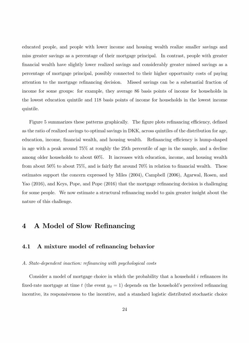
Figure 5 summarizes these patterns graphically. The figure plots refinancing effi ciency, defined
as the ratio of realized savings to optimal savings in DKK, across quintiles of the distribution for age,
education, income, financial wealth, and housing wealth. Refinancing effi ciency is hump-shaped
in age with a peak around 75% at roughly the 25th percentile of age in the sample, and a decline
among older households to about 60%. It increases with education, income, and housing wealth
from about 50% to about 75%, and is fairly flat around 70% in relation to financial wealth. These
estimates support the concern expressed by Miles (2004), Campbell (2006), Agarwal, Rosen, and
Yao (2016), and Keys, Pope, and Pope (2016) that the mortgage refinancing decision is challenging
for some people. We now estimate a structural refinancing model to gain greater insight about the
nature of this challenge.
4 A Model of Slow Refinancing
4.1 A mixture model of refinancing behavior
A. State-dependent inaction: refinancing with psychological costs
Consider a model of mortgage choice in which the probability that a household i refinances its
fixed-rate mortgage at time t (the event yit = 1) depends on the household’s perceived refinancing
incentive, its responsiveness to the incentive, and a standard logistic distributed stochastic choice
24
error εit following Luce (1959).
The refinancing probability of the household i at time t can be written as
17Standard references include Gouriéroux and Monfort (1996), Train (2009), and Cameron and Trivedi (2005).Gaudecker, Soest and Wengström (2011) and Handel (2013) are recent applications of the methods that we employ.18Mixture models have a long history in statistics since Pearson (1894). A recent survey is presented in McLachlan
and Peel (2000). Two applications where mixture models are used to uncover decision rules are El-Gamal and Grether(1995) for Bayesian updating behavior, and Harrison and Rutström (2009) for models of decision-making under risk.
26
This leads to the household log likelihood function over our sample specified as:
lnL(χ, ϕ, θi, β) =∑t
∑i
ln (Lit(χ, ϕ, θi, β)) . (14)
This framework models deviations from rational refinancing using two parameter vectors χ and
ϕ, a scalar parameter σ2θ that governs the variance of θi in equation (14), and a scalar parameter β.
The parameter vector χ captures the demographic determinants of the probability that a house-
hold is awake and responding to refinancing incentives in a given period. The parameter vector
ϕ determines whether particular demographic characteristics are associated with higher or lower
geneity in household psychological refinancing costs. Finally, the scalar parameter β determines
the responsiveness of households in each period to the modified refinancing incentive. One inter-
pretation of this parameter is that it reflects unobserved household-level shocks to the refinancing
threshold, which are uncorrelated both across households and over time.
In any cross-section these parameters determine a set of curves, each of which relates the re-
financing frequency for a household with a given set of demographic characteristics to the ADL
refinancing incentive at a point in time. The model implies that each curve has a logistic form,
close to zero for highly negative incentives and positive for highly positive incentives. The height
of the curve for highly positive incentives measures the probability that the given type of household
is awake. The horizontal position of the point where the curve reaches half this height measures
the increment to the ADL threshold implied by the average psychological refinancing costs for this
type of household. The slope of the curve at this point is governed by the parameters σ2θ and β,
which for simplicity we do not allow to vary with household demographics.
Together, the model’s parameters govern household behavior over time and tell us the relative
importance of time-dependent and state-dependent inaction in explaining failures to refinance. For
example, if the parameters ϕ and σ2θ are estimated to be zero, then there are no psychological costs
of refinancing. In this case every household will eventually refinance whenever they face a positive
ADL incentive to do so, implying that the problem is time-dependent inaction. If on the other hand
27
the parameters χ imply that households are always awake, then households will refinance whenever
they reach the threshold determined by their particular psychological refinancing costs, implying
that state-dependent inaction is the cause of refinancing failures. In the former case, a modest
decline in interest rates will eventually induce all households to refinance, whereas in the latter case
a sizeable interest rate movement is required for some households to overcome the psychological
costs that inhibit refinancing.
4.2 Comparing alternative specifications
We first explore the relative importance of the various elements of our model. Table 2 reports
parameter estimates for a series of models with an increasing number of parameters. We do not
report standard errors for the estimated parameters, since all coeffi cients are statistically significant
at the 1% level or less. Instead, we summarize the fit of each model using a pseudo R2 statistic
based on the log likelihood of the model relative to Model 4, the model which includes both state-
dependent and time-dependent inaction, restricted to be the same for all households and time
periods.
All models include the parameter β, and in Model 1, this is the sole parameter. The estimate of
β in Model 1 is −1.35, indicating that each 1 basis point change in the incentive in the neighborhood
of a zero incentive increases the refinancing probability by only 6 basis points. The relative fit of
this model is very poor, since it implies a refinancing rate that is too high on average and varies
little with refinancing incentives.
Model 2 adds a scalar psychological refinancing cost ϕ, equal for all households, to this basic
model. The fit of the model improves somewhat but the estimate of β is still very low and the
estimated ϕ = 6.13 is unreasonably high, implying a psychological refinancing cost of 457,602
DKK, or approximately $69,000.
Model 3 eliminates ϕ but adds a scalar parameter χ governing the probability that households
are asleep, which is equal for all households. The estimated magnitude of χ = 2.38 implies that
28
92% of households are asleep in any given quarter. In this model, β is estimated to be 1.30 implying
a 92 basis point response of the refinancing probability to the incentive around zero for the 8% of
households who are awake. This model fits considerably better than Model 2, another indication
that time-dependent inaction is important to explain Danish household behavior.
Model 4 includes both ϕ and χ parameters in addition to β. The fit of the model further
improves, and the estimated parameters appear sensible. Estimated ϕ = 2.44 in this model implies
a more realistic psychological cost of 11, 439 DKK, or approximately US$ 1, 716. From Table 1,
44% of the household-quarter observations are above the ADL threshold. Augmenting the ADL
threshold by 11,439 DKK implies that only 12% of household-quarters are above the augmented
threshold. The estimated magnitude of χ implies that 84% of households are asleep each quarter.
Finally, β of 0.75 implies a 47 basis point response of the refinancing probability to the incentive
around zero for the 16% of households who are awake.
Model 5 adds unobserved heterogeneity in psychological refinancing costs by estimating a free
parameter σ2θ using the MSLmethod. While this parameter, like all others in the table, is statistically
significant at the 1% level, the improvement in pseudo R2 is modest, at 0.7%.
Models 6 through 9 explore the importance of adding time effects and mortgage age effects to
the reference Model 4. These can be added either to the psychological refinancing cost ϕ or to the
asleep probability χ. Model 6 adds time effects to ϕ, and Model 7 also adds mortgage age effects
to ϕ. Model 8 instead adds time effects to χ, and Model 9 also adds mortgage age effects to χ.
Models 6 and 8 show large gains in pseudo R2 from adding time effects, implying that the
refinancing waves illustrated in Figure 3 are not simply the result of interest rate declines pushing
households across fixed thresholds, but also result from shifts over time in household responses to
incentives. However, the improvement in explanatory power is considerably greater in Model 8, at
4.1%, than in Model 6, at 2.9%. In other words, the intuitive procedure of including time effects
in the time-dependent element of the model– the probability that households are asleep– delivers
a superior fit.
29
Mortgage age effects also contribute to explanatory power, and again the fit is superior when
these effects are added to the asleep probability χ rather than the psychological refinancing cost ϕ.
Model 9, the best model considered so far, has a pseudo R2 of 5.2%.
Further gains in explanatory power are obtained by adding demographic variables. Model 10
adds demographic covariates to both ϕ and χ, increasing the pseudo R2 to 6.9%. Model 11 adds
a free parameter σ2θ to Model 10, estimating the model using the MSL method. The improvement
in pseudo R2 is extremely small at 0.1%. Given the computational burden of estimating random
coeffi cients models and the negligible improvement in fit, we drop unobserved heterogeneity in
psychological refinancing costs from further consideration and proceed with Model 10 as our base
case.
The magnitudes of the estimated parameters in Model 10 are sensible. For the reference
household in the last quarter of the sample, the estimated ϕ implies psychological refinancing costs
of 12, 768 DKK or roughly US$ 1, 914; χ implies that 96% of reference households are asleep in
this quarter; and β implies a 57 basis point response response of the refinancing probability to the
incentive around zero for reference households who are awake.19
4.3 Properties of our baseline model
We now explore in detail the ability of our baseline model (Table 2, Model 10) to fit the Danish data.
Figure 6 shows the sample distribution of incentives, together with the observed sample refinancing
probability at each incentive level. As previously discussed, most incentives are negative, but
there is a substantial fraction of positive incentives. The observed refinancing probability increases
strongly around the zero level, peaking at an incentive slightly above 1%. Very few observations
have positive incentives greater than this, so the observed sample refinancing probability at high
incentive levels is based on limited data and is correspondingly noisy.
19The reference household is an unmarried couple without children, and with no financial literacy in the householdor the extended family, living in Copenhagen with median age, education, income, wealth and housing wealth, andwith a recently issued mortgage.
30
Figure 6 also shows our model’s predicted refinancing probability, and the estimated average
probability that households in each incentive bin are awake. The model-predicted refinancing
probability captures the overall cross-sectional pattern of refinancing quite well, although it un-
derpredicts refinancings with extremely negative incentives and overpredicts refinancings with ex-
tremely positive incentives, both areas in which the data are sparse. The figure also shows that the
probability that households are awake is somewhat noisy across bins, but averages about 10% for
households with negative incentives, rises to 15% for households with low positive incentives, and
declines to about 7% for households with high positive incentives. This pattern is the result of
demographic variation in the population at each incentive level, as incentives do not directly enter
our specification for the probability that households are awake.
Figure 7 shows the estimated cross-sectional distribution of refinancing costs and their impli-
cations for the interest savings that induces refinancing. The left side of the figure measures
refinancing costs in DKK, while the right side reports the implications of these costs for the posi-
tion of the interest threshold. The top left panel shows financial refinancing costs varying from a
little over DKK 3, 000 to the upper winsorization point just below DKK 10, 000, with a mean of
DKK 5, 850. The top right panel reports the distribution of the corresponding ADL refinancing
threshold, varying from about 50 to about 250 basis points, with a mean of 83 basis points and
standard deviation of 37 basis points.
The middle left panel of Figure 7 shows the psychological refinancing costs in DKK, varying
from almost zero to about DKK 30, 000 with a mean of 10, 400. Unsurprisingly, these costs lead
to large increases in the threshold that triggers refinancing, as shown in the middle right panel
of Figure 7. Threshold increases have a mean that is comparable to the ADL threshold, but a
standard deviation that is almost twice as large. Finally, the bottom panels of Figure 7 show the
distributions of total refinancing costs and the total threshold that triggers refinancing. The total
threshold is shifted to the right and spread out by the psychological refinancing costs, with a mean
of 146 basis points and a standard deviation of 60 basis points.
A striking pattern documented in Online Appendix Table B7 is that households’ADL refi-
31
nancing thresholds are almost uncorrelated with their psychological refinancing costs in DKK, but
are strongly positively correlated with the increments to the refinancing threshold caused by those
psychological refinancing costs. The correlation between the ADL threshold and the psychological
refinancing cost is −0.02, but the correlation between the ADL threshold and the psychological
increment to the refinancing threshold is 0.87. The reason for this pattern is that refinancing costs
in DKK have a larger impact on the refinancing threshold for smaller, older mortgages as illustrated
in Figure 1. Households with these mortgages therefore tend to have both higher ADL thresholds
and higher increases in the thresholds caused by their psychological refinancing costs.
Turning to time-dependent inaction, the top panel of Figure 8 reports the cross-sectional distrib-
ution of the probability that households were asleep in a typical quarter of our sample (using sample
average time effects and mortgage age effects). There is strong time-variation in this distribution
as shown in the bottom panel of Figure 8 using a box-whisker plot. Quarters with high refinancing
activity are explained by the model not as the result of declines in interest rates that move many
households over their refinancing thresholds, but as the consequence of time fixed effects that imply
a lower probability that households are asleep in those quarters.20 Over the whole sample, the av-
erage probability that a household is asleep is 87%, with a standard deviation of 5% (that includes
both cross-sectional variation and variation over time for a given household).
Cross-sectionally, there is a strong negative correlation between the probability that a household
is asleep and psychological refinancing costs measured in monetary units. The correlation is −0.66
in a typical quarter (using sample average time effects and mortgage age effects for the asleep
probability), as reported in Online Appendix Table B7 and illustrated in Figure B10.21 The
reason, as we discuss in greater detail below, is that younger households with higher socioeconomic
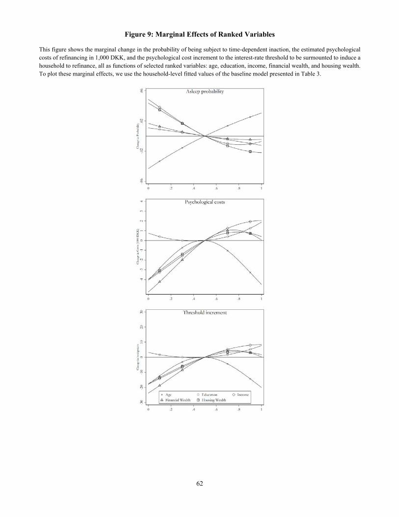
status are more likely to be awake but also have higher psychological refinancing costs in DKK.
20While time effects are not the focus of our paper, we have verified using Google Trends that internet searchactivity for Danish refinancing terms moves closely with the refinancing rate (Online Appendix Figure B8) andinversely with the cross-sectional average probability that households are asleep in each quarter (Online AppendixFigure B9). It is also possible that social interactions, of the sort measured by Maturana and Nickerson (2017),contribute to the time effect.21Online Appendix Table B8 estimates a restricted model in which the coeffi cient vectors ϕ and χ are proportional
to one another, strengthening the negative correlation between the probability that a household is asleep and itspsychological refinancing costs. This model has a pseudo R2 statistic of 6.4%, 0.5% lower than the baseline model.
32
Thus time-dependent and state-dependent inaction are strongest for different types of households.
A caveat is that this negative correlation disappears when we measure the psychological incre-
ment to the refinancing threshold. The correlation is only −0.002 between the probability that
a household is asleep and the psychological threshold increment. The discrepancy arises because
young households with high socioeconomic status tend to have larger mortgages whose refinancing
thresholds are less sensitive to the level of refinancing costs in DKK.
4.4 Cross-sectional variation in the determinants of slow refinancing
We now turn to a more detailed analysis of the mapping between Danish households’demographic
characteristics, their probability of considering a refinancing, and their psychological refinancing
costs. Table 3 reports estimates of all the demographic effects in our baseline model. Inspection
of the coeffi cients on dummy variables in Table 3 shows that some demographic characteristics are
associated with faster refinancing through both channels. Financial literacy of the household or the
family has this effect, consistent with recent work highlighting the beneficial impacts of financial
education on a range of household finance decisions (see, e.g., Haliassos, Jansson, and Karabulut,
2019), as do life events such as getting married or having children.22 On the other hand, there
are also characteristics that move people closer to the rational benchmark in one dimension but
further away in the other. For example, married couples are more likely to be awake but have
higher psychological refinancing costs than unmarried couples, while immigrants have the opposite
pattern.
Table 3 also reports the coeffi cients on ranked variables: age, education, income, financial wealth,
and housing wealth. Previous literature has suggested that such variables may have nonlinear
effects. For example Agarwal, Driscoll, Gabaix, and Laibson (2009) report nonlinear effects of age
on many financial decisions, with financial sophistication increasing among younger people as they
22The positive effect of life events on refinancing is surprising to the extent that life events raise the value of time.However, life events can induce households to reconsider and alter their financial strategies, as when married couplesmerge their bank accounts or new parents buy life insurance, and this may also stimulate refinancing.
33
gain experience, and decreasing among older people perhaps because of cognitive decline. We have
tried two different ways to model such nonlinearities, either using a piecewise linear function with a
kink at the median (achieved by adding the absolute value of the demeaned rank to the regression),
or using a quadratic function (by adding twice the squared demeaned rank, a normalization that
allows direct comparison of the coeffi cients in the two specifications). We find qualitatively similar
results with either method and report the quadratic specification in the paper.
To understand the implied marginal effects of ranked variables, Figure 9 plots the variability in
the estimated probability of being asleep, the estimated psychological costs of refinancing in DKK,
and the estimated psychological increment to the refinancing threshold, as functions of the ranked
variables. The figure is based on a two-step procedure in which the full model is used to estimate
refinancing probability, and then the fitted refinancing probability is regressed on the demographic
variables, including dummy variables, but excluding mortgage characteristics. This procedure
implies that the effects of mortgage age and size covariation with demographic characteristics are
attributed to those characteristics, rather than holding mortgage variables constant as demographic
characteristics vary. It therefore conveys a more accurate impression of how implied behavior varies
cross-sectionally in our model.
The top panel of Figure 9 shows that older households are more likely to be asleep, while
households with higher education, income, financial wealth, and housing wealth are all less likely
to be asleep. These patterns imply that a time-dependent model of inaction is consistent with the
lower refinancing effi ciency of older households and those with lower socioeconomic status that was
illustrated in Figure 5.
The cross-sectional patterns are very different for psychological refinancing costs in DKK, shown
in the middle panel of Figure 9. Middle-aged people have higher psychological refinancing costs than
younger or older people. Households with higher education, income, financial wealth, and housing
wealth all have somewhat higher psychological refinancing costs, helping to explain the negative
correlation between these costs and the probability that a household is awake. The bottom panel
of Figure 9 plots the psychological increment to the refinancing threshold rather than the costs that
34
generate that increment. The cross-sectional patterns are similar in this panel.
One plausible interpretation of these patterns is that some of the psychological DKK refinancing
costs estimated by our model correspond to the value of time spent planning and executing a
refinancing, since the monetary value of time is likely higher for middle-aged people and for people
with higher income and wealth. This interpretation can also explain the result shown in Table 3
that psychological DKK refinancing costs are higher for families with children.23
4.5 Robustness
In this section we verify that our results are not sensitive to our choice of mortgage sample, to
the parameterization of the ADL optimal refinancing model, or to our decision to use the ADL
model as our rational refinancing benchmark. We also compare the ADL threshold with the
recommendations of Danish financial advisers, and with the behavior of those Danish households
who refinance early in their cohort. Finally, we examine the robustness of our results to the logistic
functional form assumed in our stochastic choice model.
A. Alternative mortgage samples
Online Appendix C replicates Table 3 and Figures 4—6 and 8, excluding all cash-out and maturity
extension refinancing from our sample. Online Appendix D excludes households that refinance from
an FRM to an ARM from the sample, as strictly speaking, the ADL formula applies to FRM-to-
FRM refinances. Online Appendix E restricts the mortgage sample to include only mortgages with
principal value above DKK 250,000 and remaining maturity of at least 20 years. These larger and
longer-maturity mortgages have refinancing thresholds that are less sensitive to parameter inputs
and the choice of refinancing model. In all of these cases, our model delivers similar results to those
reported in the paper.
23An alternative behavioral interpretation of the middle panel of Figure 9 could be that households think ofmortgage savings in proportional terms, and wait to refinance until the interest savings exceed the rational thresholdby a given amount, regardless of the size of their mortgage. But under this interpretation all the lines in the bottompanel of Figure 9 should be flat– which is approximately true for education, but not for any of the other lines in thefigure.
35
B. Alternative parameter choices for the ADL model and behavioral refinancing model
We have explored the sensitivity of the ADL threshold to changes in the assumed parameters.
Online Appendix Figure F1 shows that a 50% reduction in the assumed interest-rate volatility σ
lowers the threshold by about 20 basis points on average, while Figure F2 shows that a 50% reduction
in the household’s discount rate ρ lowers it by less than 10 basis points. These changes are small
enough to have very little impact on our conclusions about household behavior. Unsurprisingly,
when we repeat our analysis with these two parameter modifications, in Online Appendices G and
H, we obtain similar results to those in the paper.
Online Appendix I assumes a constant mortgage termination probability of 10%, rather than
using the estimated mortgage termination probability for all households. This input to the ADL
model affects the position of the optimal refinancing threshold, but does not affect the estimates
greatly.
Online Appendix J allows demographic characteristics to affect the parameter β that governs
household responsiveness to incentives. Results in these cases are again similar to the base case.
We have also considered a model in which households are more likely to be awake when interest
rates cross discrete “round number”thresholds, but have not found any evidence of such effects.
C. Alternative model of optimal refinancing
In a more ambitious exercise, we recompute optimal refinancing thresholds using the approach
of Chen and Ling (CL 1989), which differs from the ADL approach in several substantive ways.24
The CL model treats mortgages as having a finite maturity, with an early prepayment that occurs
(in the absence of refinancing) at a known future date. The short-term interest rate is assumed to
follow a geometric Brownian motion, and a term structure model is used to derive the corresponding
24The ADL and CL models are similar in one important respect: they both assume that mortgage borrowers arerisk-neutral with respect to refinancing proceeds. We are not aware of any threshold models that allow for borrowerrisk aversion. Risk aversion would likely reduce the refinancing threshold (since refinancing today locks in an interestsaving as opposed to waiting for a potentially larger but risky saving tomorrow), which would increase our estimatesof psychological refinancing costs. However, if interest rates are positively correlated with household income, it ispossible that delaying refinancing would insure income risk, in which case risk aversion could increase the thresholdand lower our estimates of psychological refinancing costs.
36
mortgage rate.
Most importantly, in the CL model refinancing can only occur once, rather than multiple times.
Our application of the ADL model ignores the fact that under Danish rules, a refinancing today
reduces the value of future refinancing opportunities by increasing mortgage principal; but the
CL model makes future refinancing impossible, and so (setting aside other differences between the
two models), the difference between the CL and ADL thresholds provides an upper bound on the
magnitude of this effect.
The CL model does not deliver an analytical formula for the optimal refinancing threshold, so we
use numerical simulations to derive thresholds corresponding to a large number of mortgages with
given parameters (including candidate psychological refinancing costs), and interpolate thresholds
for other mortgages.
Online Appendix K discusses the CL model and our implementation of it in greater detail,
and compares the CL and ADL refinancing thresholds in our sample. We find that the average
difference between the ADL and CL thresholds is 18 basis points, the median difference is 14 basis
points, the standard deviation of the difference is 35 basis points, and the interquartile range runs
from −9 to 39 basis points. The CL and ADL thresholds have a cross-sectional correlation of 0.85.
Importantly, the differences between the two thresholds are large only for mortgages with lower
principal and shorter maturities; these mortgages have high refinancing thresholds whose exact
values are sensitive to assumptions, but for this very reason they do not play an important role in
our analysis because both the CL and ADL models imply that they should not be refinanced.25
Online Appendix L replicates Table 3 and Figures 4—6 and 8 using CL thresholds in place of
ADL thresholds. Online Appendix M repeats this exercise for the smaller sample of mortgages,
already considered in Appendix E, that have principal value above DKK 250,000 and remaining
25Among mortgages with high principal and long maturity, the correlation between the ADL and CL thresholdsis much lower. This is because such mortgages differ primarily in their exogenous termination probability, which ismodeled as a constant hazard by ADL and as a shift in a known future termination date by CL. A higher terminationprobability raises the ADL refinancing threshold, but lowers the CL threshold by reducing the value of the option towait for lower mortgage rates in the future. Appendix K discusses this phenomenon in greater detail. It does notaffect our empirical results because both the ADL and CL thresholds for mortgages of this sort are small relative tothe thresholds that trigger household refinancing in our data.
37
maturity of at least 20 years. There are some shifts in the curves relating ranked variables to
psychological costs of refinancing measured in DKK, but no other changes worthy of note.
D. Reconciliation with financial advice and prompt refinancing behavior
We complement the CL analysis with two further reality checks on the ADL refinancing thresh-
old. First, we verify that the shape of the ADL threshold illustrated in Figure 1 is broadly consistent
with the recommendations of Danish financial advisers. A typical recommendation from the real
estate advisory firm Bolius Boligejernes Videncenter (see https://www.bolius.dk/omlaegning-af-dit-
realkreditlaan-17799/) is to refinance when a) the difference between the old and the new coupon is
at least 150 basis points, b) the outstanding principal is at least DKK 250,000, and c) the remaining
time to maturity is at least 5 to 10 years. Mortgages with large outstanding principal and/or long
remaining maturity are recommended to refinance at a lower coupon differential. In our sample
period, the difference between the yield and the coupon on new mortgages is on average 36 basis
points, implying from condition a) that refinancing is advantageous when the difference between
the old coupon and the new yield is 114 basis points. In comparison the median household in our
sample has an ADL threshold of 75 basis points. While this is 39 basis points lower, we note that
the average mortgage in our sample has greater outstanding principal (DKK 926,000) and a longer
time to maturity (23 years) than the mortgage contemplated by Bolius.
Second, we check the relationship between the empirically measured incentives of prompt refi-
nancers and the ADL threshold. To ensure that we pick up individuals who respond promptly to
incentives, we conduct this exercise for loans issued in the last quarter of 2009 or later. We do so to
avoid misclassifying sluggish households from early loan cohorts as prompt refinancers during our
sample period.
For each cohort of issued loans, we define individuals as prompt refinancers if they are in the
first few percent of households to refinance in a given loan cohort. We vary this percentage cutoff,
picking the first 2.5%, 5%, and 10% of households to refinance. We measure the average incentive
for each such household, the interest saving relative to the ADL threshold, in the first quarter in
38
the time series in which the percentage cutoff is hit.26
When we average across loan cohorts using weights proportional to the number of loans issued
in each cohort, we find that prompt refinancers classified with a 2.5% cutoffhave a weighted average
incentive of 24 basis points; the 5% cutoff yields 49 basis points, and a 10% cutoff, 64 basis points.
This simple exercise produces average incentives for prompt refinancers that are quite small, which
is consistent with the ADL formula approximately capturing the rational refinancing threshold in
the Danish institutional setting. Online Appendix N provides more details about this exercise.
E. Functional form of the stochastic choice model
Finally, we explore the effect of functional form misspecification on our parameter estimates.
Online Appendix O uses a probability distortion, analogous to that used in behavioral finance
models, to alter the assumed logistic distribution of the stochastic choice error. We estimate
our model on data simulated from the misspecified model. We find that symmetric probability
distortion has minimal effect on any of the parameters of our model, while an asymmetric distortion
is picked up by our estimation procedure as an increase in the unconditional average probability
that households are asleep and the unconditional average psychological refinancing cost. However,
in no case does functional form misspecification have any major effect on the parameter estimates
that capture cross-sectional variation in time-dependent and state-dependent inaction, which are
the main concern of our paper.
4.6 Applying the model
In this section we use our model to explore the effects on refinancing of various plausible alterations
to the mortgage system in a hypothetical simulation. We consider a random sample of mortgage
26An example might make this easier to understand. The first loan cohort that we consider has an issue date of2009Q4 and contains 7,554 loans. In this cohort, 47 loans refinance in 2010Q1, 73 in 2010Q2, 398 in 2010Q3, 503 in2010Q4, and so on. The first quarter in which the 5% cutoff for prompt refinancing is exceeded is 2010Q3, in which5.2% of all loans in the 2009Q4 cohort are refinanced. Thus, households in the 2009Q4 cohort who refinanced theirmortgages in 2010Q3 are classified as “prompt”refinancers, and we calculate their average incentives in that quarterto be 8 basis points.
39
borrowers drawn from the Danish population at the start of our refinancing sample period in the
first quarter of 2010. We lower the interest rate from the actual level by 172 basis points, a decline
chosen to give 90% of the sample positive refinancing incentives relative to the ADL threshold. We
fix the interest rate at this low level for three years, and track refinancing behavior over time in
various alternative scenarios.
As a first exercise, we calculate the effects of different components of our model on aggregate
refinancing rates and the refinancing effi ciency of different types of borrowers. The top panel of
Online Appendix Figure B11 shows cumulative aggregate refinancing rates in a fully rational model
with automatic refinancing at the ADL threshold, a pure state-dependent model with rational
refinancing at the threshold augmented by our estimated psychological refinancing costs, a pure
time-dependent model in which information-gathering costs lead to rational refinancing at the ADL
threshold only by households that are awake, and finally our baseline model. Unsurprisingly
the cumulative refinancing rate for the fully rational model reaches 90% in the first quarter and
stays there, while the cumulative refinancing rate in the state-dependent model with augmented
thresholds is lower at just above 60% but has the same time pattern. A pure time-dependent
model, by contrast, has a smoothly rising cumulative refinancing rate, and our model has the same
time pattern at a lower level.
We also calculate the refinancing rates of different groups of borrowers as a fraction of the ra-
tional refinancing rates for the same groups. This is closely related to the measure of refinancing
effi ciency illustrated in Figure 3, although for simplicity we do not calculate interest savings. These
refinancing effi ciency measures can be calculated at any period of the simulation, and Online Appen-
dix Figure B11 reports results two years after the initial interest rate decline. Among households
grouped by age, state-dependent inaction lowers the refinancing effi ciency of middle-aged households
relative to younger and older households, while time-dependent inaction lowers the refinancing effi -
ciency of older households. In our full model the effect of time-dependent inaction dominates, just
as we saw in the data in Figure 5. Among households grouped by income, state-dependent inaction
lowers the refinancing effi ciency of higher-income households, while time-dependent inaction lowers
the refinancing effi ciency of poorer households. Again, time-dependent inaction dominates in both
40
the simulation and the data.
In Figure 10 we consider three modifications of the Danish mortgage system designed specifically
to improve the refinancing effi ciency of older and poorer households. These are compared with our
baseline model of the current Danish mortgage system and with fully rational refinancing at the
ADL threshold. The first modification (labeled R) rebates the fixed component of the mortgage
refinancing fee (DKK 3, 000) and removes the caps on the fees to make the mortgage refinancing
fee proportional. This eliminates the tendency of smaller mortgages (which are disproportionately
held by older and poorer households) to have higher ADL thresholds. The second modification
advertises refinancing opportunities (lowers information-gathering costs) in such a way that one-
half of all households who were asleep are woken up. The third modification combines these two
policies.
The top panel of Figure 10 shows that waking households up is a much more powerful way to
increase aggregate refinancing rates. This may not be surprising given the large size of the interest
rate reduction we are considering, which is suffi cient to give 90% of households an incentive to
refinance relative to the ADL threshold. The second and third panels similarly show that wak-
ing households up– reducing time-dependent inaction– is the best way to improve the refinancing
effi ciency of older and poorer households, although refinancing rebates do have a larger effect on
poorer households as one would expect.
These findings are relevant for the literature on the mortgage refinancing channel of monetary
transmission (Auclert 2016, Agarwal et al. 2015, Beraja et al. 2017, Di Maggio et al. 2016). Ex-
pansionary monetary policy stimulates the economy in part by lowering mortgage rates, which in
turn increases household consumption. However, in a fixed-rate mortgage system lower mortgage
rates relieve the budgets only of households that refinance their mortgages. Such budget relief
is persistent, and therefore should stimulate consumption roughly one-for-one for households that
have either no binding borrowing constraints (permanent income consumers) or fixed and binding
borrowing constraints. To the extent that budget relief relaxes borrowing constraints by permitting
households to extract home equity, or to increase uncollateralized borrowing, the effect on consump-
41
tion may initially exceed the effect on budget relief. Refinancing failures by poorer households limit
the passthrough from declining mortgage rates to consumption, and particularly do so to the extent
that poorer households are more likely to face borrowing constraints that can be relaxed by budget
relief. Policies to mitigate such refinancing failures– by reducing information-gathering costs or
even refinancing mortgages automatically– therefore have the potential to increase the effectiveness
of monetary policy stimulus during economic downturns.
5 Conclusion
In this paper we have documented slow mortgage refinancing behavior among Danish households.
The Danish context is particularly advantageous for studying this type of household behavior be-
cause the Danish mortgage system places no restrictions on refinancing that does not involve cash-
out, so households that pass up opportunities to substantially reduce their mortgage costs are not
constrained, but are making mistakes in managing their finances. In addition, the Danish statistical
system allows us to measure the demographic and economic characteristics of households in great
detail.
We distinguish between time-dependent and state-dependent models of slow refinancing. A
time-dependent model has a reduced probability of refinancing at any incentive, while a state-
dependent model increases the threshold that triggers refinancing, equivalent to the addition of
psychological costs to the direct financial costs of refinancing. We demonstrate that while a pure
state-dependent model can fit any observed behavior in a single cross-section of the data, it imposes
strong restrictions in a panel that are rejected in the data. We therefore build a model which allows
for both sources of inaction to affect refinancing decisions.
We find that older households and those with lower education, income, housing wealth, and
financial wealth are all strongly affected by time-dependent inaction, whereas the psychological
refinancing costs that create state-dependent inaction are greatest for middle-aged households and
those with high financial wealth. The cross-sectional variation in psychological refinancing costs
42
is consistent with the view that these costs may in part capture the high value of time for certain
households. Time-dependent slow refinancing is the primary reason why older households and
those with lower socioeconomic status achieved low interest savings from refinancing during our
sample period, relative to the savings achievable with an optimal refinancing strategy.
One might be concerned that these patterns are sensitive to the ADL formula we have used
as our rational benchmark for refinancing. To address this concern, we have shown that Danish
households who refinance promptly (in the first few percent of households whose old mortgages
carry the same interest rate) do so at interest savings similar to the ADL threshold. We have also
recomputed all thresholds using an alternative model of optimal refinancing due to Chen and Ling
(1989), and obtain similar results. Our conclusion is that while different assumptions can have
noticeable effects on optimal refinancing thresholds, they cannot make a large enough difference
to account for the slow refinancing rates observed in the Danish data or to substantially alter the
cross-sectional patterns in time- and state-dependent refinancing that we document.
Both our methodology and our findings have relevance beyond the context of this paper. We
believe that the mixture model we have used to estimate time-dependent slow refinancing is a
promising econometric method for estimating the prevalence of behavioral biases in the population,
and a useful alternative to the competing-risks proportional hazard framework of Deng, Quigley,
and Van Order (2000) for modeling heterogeneous prepayment behavior. Our findings reinforce
concerns that financial capabilities deteriorate late in life (Agarwal, Driscoll, Gabaix, and Laibson
2009) and that poorer households make worse financial decisions (Campbell 2006, Calvet, Campbell,
and Sodini 2009b, Badarinza, Campbell, and Ramadorai 2016), contributing to inequality of wealth
(Piketty 2014, Bach, Calvet, and Sodini 2015, Campbell 2016). Finally, our results imply that the
effect of expansionary monetary policy on household consumption is weakened in economies with
predominantly fixed-rate mortgages, not only by barriers to refinancing that may result from low
credit scores and house prices, as emphasized by Agarwal et al. (2015), Beraja et al. (2017), and Di
Maggio et al. (2016), but also by the slow reaction of many households to refinancing opportunities.
43
References
Abel, Andrew B., Janice C. Eberly, and Stavros Panageas, 2007, “Optimal Inattention to theStock Market”, American Economic Review: Papers and Proceedings 97, 244—249.
Abel, Andrew B., Janice C. Eberly, and Stavros Panageas, 2013, “Optimal Inattention to theStock Market with Information Costs and Transactions Costs”, Econometrica 81, 1455—1481.
Agarwal, Sumit, Gene Amromin, Souphala Chomsisengphet, Tomasz Piskorski, Amit Seru, andVincent Yao, 2015, “Mortgage Refinancing, Consumer Spending and Competition: Evidencefrom the Home Affordable Refinancing Program”, NBER Working Paper 21512.
Agarwal, Sumit, John Driscoll, and David Laibson, 2013, “Optimal Mortgage Refinancing: AClosed Form Solution”, Journal of Money, Credit, and Banking 45, 591—622.
Agarwal, Sumit, John Driscoll, Xavier Gabaix, and David Laibson, 2009, “The Age of Reason:Financial Decisions Over the Life Cycle and Implications for Regulation”, Brookings Paperson Economic Activity 2, 51—101.
Agarwal, Sumit, Richard J. Rosen, and Vincent Yao, 2016, “Why Do Borrowers Make MortgageRefinancing Mistakes?”, Management Science 62, 3494—3509.
Agnew, Julie, Pierluigi Balduzzi, and Annika Sunden, 2003, “Portfolio Choice and Trading in aLarge 401(k) Plan”, American Economic Review 93, 193—215.
Alvarez, Fernando, Luigi Guiso, and Francesco Lippi, 2012, “Durable Consumption and AssetManagement with Transaction and Observation Costs”, American Economic Review 102,2272—2300.
Alvarez, Fernando, Francesco Lippi, and Luigi Paciello, 2011, “Optimal Price Setting With Ob-servation and Menu Costs”, Quarterly Journal of Economics 126, 1909—1960.
Anagol, Santosh, Vimal Balasubramaniam, and Tarun Ramadorai, 2018, “Endowment Effects inthe Field: Evidence from India’s IPO Lotteries”, forthcoming Review of Economic Studies.
Andersen, Steffen, John Y. Campbell, Kasper Meisner Nielsen, and Tarun Ramadorai, 2019, “Ap-pendix to Sources of Inaction in Household Finance”, available online at authors’websites.
Archer, Wayne R., David C. Ling, and Gary A. McGill, 1996, “The Effect of Income and CollateralConstraints on Residential Mortgage Terminations”, Regional Science and Urban Economics26, 235—261.
Auclert, Adrien, 2016, “Monetary Policy and the Redistribution Channel”, unpublished paper,Stanford University.
Bach, Laurent, Laurent E. Calvet, and Paolo Sodini, 2015, “Rich Pickings? Risk, Return, andSkill in the Portfolios of the Wealthy”, unpublished paper, Swedish House of Finance, EDHECBusiness School, and Stockholm School of Economics.
44
Badarinza, Cristian, John Y. Campbell, and Tarun Ramadorai, 2016, “International ComparativeHousehold Finance”, Annual Review of Economics 8, 111—144.
Badarinza, Cristian, John Y. Campbell, and Tarun Ramadorai, 2017, “What Calls to ARMs?International Evidence on Interest Rates and the Choice of Adjustable Rate Mortgages,”forthcoming Management Science.
Bajo, Emanuele and Massimiliano Barbi, 2016, “Out of Sight, Out of Mind: Media Coverage,Financial Literacy, and Mortgage Refinancing”, unpublished paper, University of Bologna.
Bennett, Paul, Richard Peach, and Stavros Peristiani, 2001, “Structural Change in the MortgageMarket and the Propensity to Refinance”, Journal of Money, Credit, and Banking 33, 955—975.
Beraja, Martin, Andreas Fuster, Erik Hurst, and Joseph Vavra, 2017, “Regional Heterogeneityand Monetary Policy”, NBER Working Paper 23270.
Bhutta, Neil, Andreas Fuster, and Aurel Hizmo, 2018, “Paying Too Much? Price Dispersion in theUS Mortgage Market”, unpublished paper, Federal Reserve Board and Swiss National Bank.
Bhutta, Neil and Benjamin J. Keys, 2016, “Interest Rates and Equity Extraction During theHousing Boom”, American Economic Review 106, 1742—1774.
Bilias, Yannis, Dimitris Georgarakos, and Michael Haliassos, 2010, “Portfolio Inertia and StockMarket Fluctuations”, Journal of Money, Credit and Banking 42, 715—742.
Brueckner, Jan K. and James R. Follain, 1988, “The Rise and Fall of the ARM: An EconometricAnalysis of Mortgage Choice,”Review of Economics and Statistics 70, 93—102.
Brunnermeier, Markus K. and Stefan Nagel, 2008, “Do Wealth Fluctuations Generate Time-Varying Risk Aversion? Micro-Evidence on Individuals”, American Economic Review 98,713—736.
Bucks, Brian and Karen Pence, 2008, “Do Borrowers Know Their Mortgage Terms?”, Journal ofUrban Economics 64, 218—233.
Caballero, Ricardo J. and Eduardo M. Engel, 1991, “Dynamic (S,s) Economics”, Econometrica59, 1659—1686.
Calvet, Laurent, John Y. Campbell, and Paolo Sodini, 2009a, “Fight or Flight? Portfolio Rebal-ancing by Individual Investors”, Quarterly Journal of Economics 124, 301—348.
Calvet, Laurent, John Y. Campbell, and Paolo Sodini, 2009b, “Measuring the Financial Sophisti-cation of Households”, American Economic Review Papers and Proceedings 99, 393—398.
Calvo, Guillermo A., 1983, “Staggered Prices in a Utility-Maximizing Framework”, Journal ofMonetary Economics 12, 383—398.
45
Cameron, A. Colin, and Trivedi, Pravin K., 2005, Microeconometrics: Methods and Applications,Cambridge University Press, New York, NY.
Campbell, John Y., 2006, “Household Finance”, Journal of Finance 61, 1553—1604.
Campbell, John Y., 2013, “Mortgage Market Design”, Review of Finance 17, 1—33.
Campbell, John Y., 2016, “Restoring Rational Choice: The Challenge of Consumer FinancialRegulation”, American Economic Review: Papers and Proceedings 106(5):1—30.
Campbell, John Y. and Joao Cocco, 2003, “Household Risk Management and Optimal MortgageChoice”, Quarterly Journal of Economics 118, 1449—1494.
Campbell, John Y. and Joao Cocco, 2015, “A Model of Mortgage Default”, Journal of Finance70, 1495—1554.
Caplin, Andrew, 2016, “Measuring and Modeling Attention”, Annual Review of Economics 8,379—403.
Caplin, Andrew, Charles Freeman, and Joseph Tracy, 1997, “Collateral Damage: RefinancingConstraints and Regional Recessions”, Journal of Money, Credit, and Banking 29, 496—516.
Caplin, Andrew and John Leahy, 1991, “State-Dependent Pricing and the Dynamics of Moneyand Output”, Quarterly Journal of Economics 106, 683—708.
Caplin, Andrew and Daniel F. Spulber, 1987, “Menu Costs and the Neutrality of Money”, Quar-terly Journal of Economics 102, 703—725.
Chen, Andrew and David Ling, 1989, “Optimal Mortgage Refinancing with Stochastic InterestRates”, AREUEA Journal 17, 278—99.
Chen, Hui, Michael Michaux, and Nikolai Roussanov, 2013, “Houses as ATMs? Mortgage Refi-nancing and Macroeconomic Uncertainty”, unpublished paper, MIT, USC, and University ofPennsylvania.
Choi, James J., David Laibson, Brigitte Madrian, and Andrew Metrick, 2002, “Defined Contribu-tion Pensions: Plan Rules, Participant Decisions, and the Path of Least Resistance”, in JamesPoterba ed. Tax Policy and the Economy 16, 67—113.
Choi, James J., David Laibson, Brigitte Madrian, and Andrew Metrick, 2004, “For Better or forWorse: Default Effects and 401(k) Savings Behavior”, in David Wise ed. Perspectives on theEconomics of Aging, University of Chicago Press.
DellaVigna, Stefano, and JoshuaM. Pollet, 2007, “Demographics and Industry Returns”, AmericanEconomic Review 97, 1667—1702.
Deng, Yongheng and John M. Quigley, 2012, “Woodhead Behavior and the Pricing of ResidentialMortgages”, unpublished paper, National University of Singapore and University of CaliforniaBerkeley.
46
Deng, Yongheng, John M. Quigley and Robert Van Order, 2000, “Mortgage Terminations, Het-erogeneity, and the Exercise of Mortgage Options”, Econometrica 68, 275—307.
Dhillon, Upinder S., James D. Shilling, and C.F. Sirmans, 1987, “Choosing Between Fixed andAdjustable Rate Mortgages: Note”, Journal of Money, Credit, and Banking 19, 260—267.
Di Maggio, Marco, Amir Kermani, Benjamin Keys, Tomasz Piskorski, Rodney Ramcharan, AmitSeru, and Vincent Yao, 2016, “Monetary Policy Pass-Through: Mortgage Rates, HouseholdConsumption and Voluntary Deleveraging”, forthcoming American Economic Review.
Duffi e, Darrell, and Tong-sheng Sun, 1990, “Transactions Costs and Portfolio Choice in a Discrete-Continuous-Time Setting”, Journal of Economic Dynamics and Control 14, 35—51.
El-Gamal, Mahmoud A. and David M. Grether, 1995, “Are People Bayesian? Uncovering Behav-ioral Strategies”, Journal of the American Statistical Association 90, 1137—1145.
Gabaix, Xavier, Arvind Krishnamurthy, and Olivier Vigneron, 2007, “Limits of Arbitrage: Theoryand Evidence from the Mortgage-Backed Securities Market”, Journal of Finance 62, 557—595.
Gabaix, Xavier and David I. Laibson, 2002, “The 6D Bias and the Equity-Premium Puzzle,” inBen S. Bernanke and Kenneth S. Rogoff eds. NBER Macroeconomics Annual 2001, MITPress, Cambridge, MA, 257—312.
Gaudecker, Hans-Martin von, Arthur van Soest, and Erik Wengstrom, 2011, “Heterogeneity inRisky Choice Behavior in a Broad Population”, American Economic Review 101, 664—694.
Gouriéroux, Christian, and Monfort, Alain, 1996, Statistics and Econometric Models, CambridgeUniversity Press, Cambridge, UK.
Gyntelberg, J., Kjeldsen, K., Baekmand Nielsen, M., and Persson, M., 2012, “The 2008 FinancialCrisis and the Danish Mortgage Market”, in A. Bardhan, R.H. Edelstein, and C.A. Kroll eds.Global Housing Markets: Crises, Policies, and Institutions, John Wiley, 53—68.
Haliassos, Michael, Thomas Jansson, and Yigitcan Karabulut, 2019, “Financial Literacy Exter-nalities,”forthcoming Review of Financial Studies.
Hall, Arden, 2000, “Controlling for Burnout in Estimating Mortgage Prepayment Models”, Journalof Housing Economics 9, 215—232.
Handel, Benjamin R., 2013, “Adverse Selection and Inertia in Health Insurance Markets: WhenNudging Hurts”, American Economic Review 103, 2643—2682.
Johnson, Kathleen W. and Geng Li, 2014, “Are Adjustable-Rate Mortgage Borrowers BorrowingConstrained?,”Real Estate Economics 42, 457—471.
Harrison, Glenn W. and E. Elisabet Rutström, 2009, “Expected Utility Theory and ProspectTheory: One Wedding and a Decent Funeral,”Experimental Economics 12, 133—158.
47
Johnson, Eric, Stephan Meier, and Olivier Toubia, 2015, “Leaving Money on the Kitchen Table:Exploring Sluggish Mortgage Refinancing Using Administrative Data, Surveys, and FieldExperiments”, unpublished paper, Columbia Business School.
Kang, Pan and Stavros A. Zenios, 1992, “Complete Prepayment Models for MBS”, ManagementScience 38, 1665—1685.
Keys, Benjamin J., Devin G. Pope, and Jaren C. Pope, 2016, “Failure to Refinance”, Journal ofFinancial Economics 122, 482—499.
Khandani, Amir E., Andrew W. Lo, and Robert C. Merton, 2013, “Systemic Risk and the Refi-nancing Ratchet Effect”, Journal of Financial Economics 108, 29—45.
Koijen, Ralph S.J., Van Hemert, Otto and Stijn Van Nieuwerburgh, 2009, “Mortgage Timing,”Journal of Financial Economics 93, 292—324.
LaCour-Little, Michael, 1999, “Another Look at the Role of Borrower Characteristics in PredictingMortgage Prepayments”, Journal of Housing Research 10, 45—60.
Laibson, David, 1997, “Golden Eggs and Hyperbolic Discounting”, Quarterly Journal of Economics112, 443—478.
Lea, M., 2011, “Alternative Forms of Mortgage Finance: What Can We Learn from Other Coun-tries?”in N. Retsinas and E. Belsky eds., Moving Forward: The Future of Consumer Creditand Mortgage Finance, Joint Center for Housing Studies, Harvard University, Cambridge,MA, and Brookings Institution Press, Washington, DC, 118—149.
Luce, R. Duncan, 1959, Individual Choice Behavior: A Theoretical Analysis, Wiley, New York,NY.
Madrian, Brigitte and Dennis Shea, 2001, “The Power of Suggestion: Inertia in 401(k) Participa-tion and Savings Behavior”, Quarterly Journal of Economics 66, 1149—1188.
Matejka, Filip and Alisdair McKay, 2015, “Rational Inattention to Discrete Choices: A NewFoundation for the Multinomial Logit Model”, American Economic Review 105, 272—298.
Maturana, Gonzalo and Jordan Nickerson, 2017, “Teachers Teaching Teachers: The Role of Net-works on Financial Decisions”, unpublished paper, Emory University and Boston College.
McConnell, John J., and Manoj Singh, 1994, “Rational Prepayments and the Valuation of Collat-eralized Mortgage Obligations”, Journal of Finance 49, 891—921.
McLachlan, Geoffrey and David Peel, 2000, Finite mixture models, Wiley, New York, NY.
Miles, David, 2004, The UK Mortgage Market: Taking a Longer-term View, HM Treasury, London,UK.
48
Moscarini, Giuseppe, 2004, “Limited Information Capacity as a Source of Inertia”, Journal ofEconomic Dynamics and Control 28, 2003—2035.
Nakamura, Emi, and Jon Steinsson, 2010, “Monetary Non-Neutrality in a Multisector Menu CostModel”, Quarterly Journal of Economics 125, 961—1013.
O’Donoghue, Ted, and Matthew Rabin, 1999, “Doing it Now or Later”, American EconomicReview 89, 103—124.
Pearson, Karl, 1894, “Contributions to the Mathematical Theory of Evolution”, PhilosophicalTransactions of the Royal Society of London A, 71—110.
Piketty, Thomas, 2014, Capital in the 21st Century, Harvard University Press, Cambridge, MA.
Schwartz, Eduardo S., and Walter N. Torous, 1989, “Prepayment and the Valuation of Mortgage-Backed Securities”, Journal of Finance 44, 375—392.
Sims, Christopher A., 2003, “Implications of Rational Inattention”, Journal of Monetary Eco-nomics 50, 665—690.
Stanton, Richard, 1995, “Rational Prepayment and the Valuation of Mortgage-Backed Securities”,Review of Financial Studies 8, 677—708.
Taylor, John B., 1980, “Aggregate Dynamics and Staggered Contracts”, Journal of Political Econ-omy 88, 1—23.
Tracy, Joseph and Joshua Wright, 2012, “Payment Changes and Default Risk: The Impact ofRefinancing on Expected Credit Losses”, Federal Reserve Bank of New York StaffReport No.562.
Train, Kenneth E., 2009, Discrete Choice Methods with Simulation, Cambridge University Press,New York, NY.
Veldkamp, Laura, 2011, Information Choice in Macroeconomics and Finance, Princeton UniversityPress, Princeton, NJ.
Veronesi, Pietro, 2010, Fixed Income Securities: Valuation, Risk, and Risk Management, JohnWiley & Sons, Hoboken, NJ.
Woodward, Susan E., and Robert E. Hall, 2010, “Consumer Confusion in the Mortgage Market:Evidence of Less Than a Perfectly Transparent and Competitive Market”, American EconomicReview 100, 511—515.
Woodward, Susan E. and Robert E. Hall, 2012, “Diagnosing Consumer Confusion and Sub-OptimalShopping Effort: Theory and Mortgage Market Evidence”, American Economic Review 102,3249—3276.
Zandi, Mark and Cristian deRitis, 2011, “Improved HARP Will Expand Refinancing, Boost Re-covery”, unpublished report, Moody’s Analytics.
Zhu, Jun, 2012, “Refinance and Mortgage Default: An Empirical Analysis of the HARP’s Impacton Default Rates”, unpublished paper, Freddie Mac.
50
51
Table 1: Characteristics of Danish Fixed Rate Mortgages
These statistics are calculated using all unique mortgages taken by households in Denmark with an unchanging number of adult members, and with a single fixed rate mortgage. In Panel A, the rows show, in order, the total number of household-quarter observations in the data; the average principal remaining (outstanding) on these mortgages in millions of Danish Kroner (DKK); the average number of years remaining before mortgages mature; the average loan-to-value (LTV) ratio on these mortgages; the fraction refinancing in a quarter (i.e., the fraction of households that refinanced their pre-existing mortgage voluntarily rather than refinancing for exogenous reasons such as moving house); the fraction refinancing from a fixed rate mortgage (FRM) to another FRM; the fraction of all mortgages with negative refinancing incentives calculated using Agarwal et al. (2013) formula (ADL); the fraction of mortgages with negative ADL incentives which refinance; the fraction of mortgages with positive refinancing incentives computed using the ADL formula; and the fraction with positive ADL incentives which refinance. In Panel B, the rows document the fractions of households refinancing either once or multiple times during the sample period. The columns document the fractions of these households refinancing at incentives which are either greater than, or less than or equal to, incentive levels previously experienced over the sample period.
Panel A: Household quarter observations Number of observations 9,351,183 Principal remaining (million DKK) 0.983 Years remaining on mortgage 23.226 Loan-to-value (LTV) ratio 0.600 Fraction refinancing 0.040 Fixed rate to fixed rate refinancing 0.701 Fraction with negative ADL incentive 0.563 - of which refinance 0.013 Fraction with positive ADL incentive 0.437 - of which refinance 0.076
Panel B: Household observations
All At higher incentives
At lower incentives
Number of households 614,811 - fraction never refinancing 0.498 - fraction refinancing once 0.402 0.276 0.126 - fraction refinancing twice 0.089 0.040 0.049 - fraction refinancing three or more times 0.011 0.002 0.009
52
Table 2: Choice Models
We estimate our random coefficient specification using all households in Denmark with an unchanging number of household members, with a single fixed rate mortgage in the beginning of each year from 2010-2017. The dependent variable takes the value of 1 if there is refinancing in a given quarter, and 0 otherwise. Each column lists the parameters of our model of refinancing: χ is the probability that a household is asleep and does not respond to refinancing incentives (i.e., probability = exp(χ)/(1+ exp(χ))). φm captures the average level of psychological refinancing costs, and depending on the model variation listed in the rows, χ and φm can be functions of demographic characteristics, and χ can also depend on mortgage age effects and current quarter effects. φsd, when included, estimates a random coefficient model for psychological refinancing costs. exp(β) captures responsiveness to incentives. Pseudo R2 is calculated using the formula R2 = 1- L1/L0, where L1 is the log likelihood from the model specified in the column header, and L0 is the log likelihood from a model which only allows for a constant probability of being asleep, a stochastic choice error, and a constant fixed psychological refinancing cost (i.e., Model 4). All coefficients in the table are significant at the 1% level or less.
Model 1 Model 2 Model 3 Model 4 Model 5 Model 6 Model 7 Model 8 Model 9 Model 10 Model 11
β* -1.350 -1.063 1.298 0.745 0.846 0.655 0.667 0.677 0.770 0.820 0.873 φm 6.126 2.437 3.289 3.149 3.785 2.465 2.219 2.547 2.580 - Current quarter dummies No No No Yes Yes No No No No - Mortgage age dummies No No No No Yes No No No No
- Demographics No No No No No No No Yes Yes φsd 1.300 0.848 χ***** 2.381 1.671 0.967 1.387 1.392 2.238 3.049 3.059 2.988 - Current quarter dummies No No No No No Yes Yes Yes Yes - Mortgage age dummies No No No No No No Yes Yes Yes - Demographics No No No No No No No Yes Yes Pseudo R2 -3.508 -0.096 -0.019 0.000 0.007 0.029 0.035 0.041 0.052 0.069 0.070
53
Table 3: Model with Heterogenous Household Characteristics
We estimate this specification using all households in Denmark with an unchanging number of household members, with a single fixed rate mortgage in the beginning of each year from 2010-2017. The dependent variable takes the value of 1 for a refinancing in a given quarter, and 0 otherwise. Each column lists the parameters of our model of refinancing: χ is the probability that a household is asleep and does not respond to refinancing incentives, and the rows show its dependence on the listed demographic characteristics. φ captures the level of psychological refinancing costs (i.e., costs = exp(φ)) once again as a function of demographic characteristics, and exp(β), which does not depend on demographics, captures the responsiveness to the incentives. The coefficients include non-linear transformations, f(x), of all the ranked control variables in addition to their levels, where f(x) = √2 . Pseudo R2 is calculated using the formula R2 = 1- L1/L0, where L1
is the log likelihood from the given model and L0 is the log likelihood from a model which only allows for a constant probability of being asleep. ***, **, and * indicate coefficients that are significant at the one, five, and ten percent level, respectively, using standard errors clustered at the level of households.
β** φ*** χ*****
Intercept 0.820*** 2.547*** 3.059*** Random coefficient component Single male household -0.088*** 0.008*** Single female household -0.106*** -0.107*** Married household 0.101*** -0.039*** Children in family 0.112*** 0.101*** Immigrant -0.101*** 0.163*** Financially literate -0.160*** -0.018*** Family financially literate -0.001*** -0.093*** Getting married -0.248*** -0.070*** Having children -0.106*** -0.087*** Region of Northern Jutland 0.112*** -0.280*** Region of Middle Jutland 0.082*** -0.215*** Region of Southern Denmark 0.024*** -0.100*** Region of Zealand 0.064*** 0.142*** Demeaned rank of: Age -0.094*** 0.783*** Length of education 0.110*** -0.251*** Income 0.815*** -0.763*** Financial wealth 0.906*** -0.242*** Housing wealth 0.636*** -0.814*** Non-linear transformation f(x), x is the demeaned rank of: Age -1.323*** -0.014*** Length of education 0.275*** -0.005**** Income -0.401*** 0.615*** Financial wealth -0.896*** 0.150*** Housing wealth -0.546*** 0.380*** Current quarter dummies Yes* Mortgage age dummies Yes* Pseudo R2 0.069 Log likelihood -1,332,195 **** Observations 9,351,183 **
54
Figure 1: ADL Threshold as a Function of Fixed Costs
This figure plots the ADL threshold level in basis points associated with each fixed cost in DKK on the x-axis. The solid line in the plot shows this mapping when the ADL threshold is computed using the mean estimated mortgage termination probability, the mean remaining mortgage principal, the mean remaining horizon on the mortgage, the mean interest rate on the mortgage, and the mean inflation rate. The two dashed lines in the plot show this mapping for (i) a smaller mortgage that is half the mean principal, and (ii) a shorter duration mortgage with half the mean remaining horizon to maturity.
55
Figure 2: Evaluating Refinancing Activity relative to the ADL threshold
This figure illustrates refinancing activity in the sample evaluated against the household-quarter-specific ADL threshold. The top plot shows the histogram of computed incentives with the refinancing probability superimposed on it; the second plot shows the number of refinancings at each point corresponding to the dark line on the top plot; and the third plot shows the Kaplan-Meier “survival” (i.e., non-refinancing) estimate, i.e., plotting the number of quarters at which the household has positive incentives but does not refinance, accounting for data censoring.
56
Figure 3: Refinancing Activity by pre-existing Mortgage Coupon Rates
This figure illustrates the history of refinancing activity in the sample of Danish fixed-rate mortgages. In the top plot, the bars represent the number of refinancing households in each quarter. The bars are shaded according to the coupon rate on the old mortgage from which households refinance. In the bottom plot, we show the evolution of the quarterly Danish mortgage interest rate as it moves through the average refinancing threshold for mortgages with a specific coupon rate. For example, the very top lightest shaded horizontal line in the bottom plot shows the average interest rate refinancing threshold for the group of mortgages that bear coupon rates of 6%, i.e., the point at which the current interest rate needs to be, on average, to optimally justify refinancing for this group of mortgage holders. The thresholds for mortgages with coupons of 6%, 5%, 4%, 3.5%, 3%, and 2.5% are 5.06%, 4.22%, 3.27%, 2.83%, 2.28%, and 1.83% respectively.
57
Figure 4: Evaluating whether Refinancing Activity occurs at a Household-specific Threshold
This figure illustrates refinancing activity to check whether households have idiosyncratic thresholds at which they always refinance. The top plot shows the histogram of the difference between computed incentives at the point at which households refinance and the best ever incentive experienced over the sample period prior to the point of refinancing; the second plot focuses on households that refinance at least twice, and plots the histogram across these households of the difference between the incentives at the two refinancing points; and the third plot shows the Kaplan-Meier “survival” (i.e., non-refinancing) estimate, i.e., plotting the number of quarters at which the household has incentives above those which they previously refinanced at but do not subsequently refinance, accounting for data censoring.
58
Figure 5: Refinancing Efficiency
This figure plots the average refinancing efficiency, calculated as the ratio of actual savings to counterfactual savings (counterfactual estimated under optimal refinancing), as a function of the ranked variables of age, education, income, financial wealth and housing wealth.
59
Figure 6: Refinancing, Incentives and Model Implied Refinancing Probabilities.
This figure plots refinancing probabilities from the baseline model presented in Table 3, as a function of refinancing incentives, alongside the number of observations at each level of incentives. The bars in this figure show the number of household-quarters (scale on the left vertical axis) and the lines show the fraction of these household-quarters that refinance (scale on the right vertical axis), both plotted for each level of refinancing incentives shown on the horizontal axis. The bars are 20-basis-point incentive intervals centered at the points on the horizontal axis. The solid line shows the actual refinancing probability observed in the data, the long-dashed line shows the model-predicted refinancing probability, and the short-dashed line shows the fraction of households that the model estimates do not perceive incentives (i.e., time-dependent inaction) in each period.
60
Figure 7: Refinancing Cost Components
These figures summarize the costs of refinancing estimated from the baseline model presented in Table 3 over the entire sample period. The three plots in the left column show the costs in 1,000 DKK, while the three plots in the right column show these costs in the form of the implied interest rate threshold in basis points that they translate into using the ADL (2013) function. Descending vertically, the first row shows the pure financial costs of refinancing, which are based on mortgage size. The second row shows the estimated psychological costs of refinancing, while the third row is the total costs, which sum the two rows above it.
61
Figure 8: Model Implied Time-Dependent Inaction Probability
This figure shows the model implied probability of households being subject to time-dependent inaction, estimated using the model in Table 3. The top panel shows a histogram of the distribution of the estimated time-dependent inaction probability across households, computed using a representative quarter, i.e., inputting the average mortgage age effect and average current quarter time effect estimated in the data. The bottom panel shows a box plot of the model implied estimated time-dependent inaction probability for each quarter of our data, i.e., inputting the time effect and mortgage age effect for each quarter listed on the vertical axis.
62
Figure 9: Marginal Effects of Ranked Variables
This figure shows the marginal change in the probability of being subject to time-dependent inaction, the estimated psychological costs of refinancing in 1,000 DKK, and the psychological cost increment to the interest-rate threshold to be surmounted to induce a household to refinance, all as functions of selected ranked variables: age, education, income, financial wealth, and housing wealth. To plot these marginal effects, we use the household-level fitted values of the baseline model presented in Table 3.
63
Figure 10: Policy Experiments
These figures consider policies to induce household refinancing alongside an interest rate cut in which 90% of Danish households have a refinancing incentive exceeding their ADL (2013) threshold: a policy in which mortgages automatically refinance when the interest rate saving exceeds the ADL threshold; a policy that “wakes up” households, cutting the asleep probability in half from its initial level; a policy that rebates all fixed fees incurred by households; a policy that combines “waking up” with the rebate; and a “do nothing policy” in which households refinance according to our baseline model. The top panel shows the fraction refinancing at each point in time, and the second (third) the fraction refinancing 8 quarters post-cut along the age (income) distribution.