Sources of Inaction in Household Finance:Evidence from the Danish Mortgage Market

Steffen Andersen, John Y. Campbell, Kasper Meisner Nielsen,and Tarun Ramadorai1

First draft: July 2014This version: March 2018

1Andersen: Department of Finance, Copenhagen Business School, Porcelaenshaven 16A, DK-2000Frederiksberg, Denmark, Email: sa.eco@cbs.dk. Campbell: Department of Economics, Littauer Cen-ter, Harvard University, Cambridge MA 02138, USA, and NBER. Email: john_campbell@harvard.edu.Nielsen: Hong Kong University of Science and Technology, Clear Water Bay, Hong Kong SAR, China.Email: nielsen@ust.hk. Ramadorai: Imperial College, London SW7 2AZ, UK, and CEPR. Email:t.ramadorai@imperial.ac.uk. An earlier version of this paper was circulated under the title “Inattentionand Inertia in Household Finance: Evidence from the Danish Mortgage Market”. We thank the SloanFoundation for financial support. We are grateful to the Association of Danish Mortgage Banks (ADMB)for providing data and facilitating dialogue with the individual mortgage banks, and to senior economistsBettina Sand and Kaare Christensen at the ADMB for providing us with valuable institutional details. Wethank Sumit Agarwal, Joao Cocco, John Driscoll, Xavier Gabaix, Samuli Knüpfer, David Laibson, TomaszPiskorski, Tano Santos, Antoinette Schoar, Amit Seru, Susan Woodward, Vincent Yao, and seminar par-ticipants at the Board of Governors of the Federal Reserve/GFLEC Financial Literacy Seminar at GeorgeWashington University, the NBER Summer Institute Household Finance Meeting, the Riksbank-EABCNConference on Inequality and Macroeconomics, the American Economic Association 2015 Meeting, the RealEstate Seminar at UC Berkeley, the Federal Reserve Bank of New York, Copenhagen Business School,Columbia Business School, the May 2015 Mortgage Contract Design Conference, the NUS-IRES Real EstateSymposium, Chicago Booth, the European Finance Association 2015 Meeting, the FIRS 2016 Meeting, theImperial College London-FCA Conference on Mortgage Markets, Cass Business School, the Banca d’Italia,Wharton, Boston College, Stanford, the 2017 Conference on the Econometrics of Financial Markets, Boc-coni, and Lugano for many useful comments, and Josh Abel and Federica Zeni for excellent and dedicatedresearch assistance.

Abstract

A common problem in household finance is that households are often inactive in response toincentives. Mortgages are generally the largest household liability, and mortgage refinancingis an important channel for monetary policy transmission, so inactivity in this setting canbe socially costly. We study how the Danish population responds to mortgage refinancingincentives between 2010 and 2014, building an empirical model that separately estimatestime-dependent inaction (a low probability of responding to a refinancing incentive in agiven quarter), and state-dependent inaction (a psychological addition to the financial costof refinancing). Psychological costs of refinancing are hump-shaped in age and generallyincreasing in socioeconomic status, consistent with the view that these costs may partlyreflect the value of time spent refinancing. The probability of responding to any incentive islowest for older households and households with low income, education, housing wealth, andfinancial wealth. Thus time-dependent inaction is the key determinant of low refinancingamong households with low socioeconomic status. Our model highlights the importance ofpolicies to make such households aware of refinancing opportunities or to refinance mortgagesautomatically.

1 Introduction

A pervasive finding in studies of household financial decision-making is that households re-

spond slowly to changing financial incentives. Inaction is common, even in circumstances

where market conditions are changing continuously, and actions often occur long after the

incentive to take them has first arisen. Well known examples include participation, saving,

and asset allocation decisions in retirement savings plans, and portfolio rebalancing in re-

sponse to fluctuations in risky asset prices.2 In this paper we study mortgage refinancing– a

particularly important decision given the size of mortgages relative to household budgets–

with a view towards shedding light on the underlying structural determinants of inaction.

We do so in Denmark, an environment uniquely suited to analyzing these questions, using a

large sample of high-quality administrative data.

One explanation for inaction is that households monitor their financial circumstances

intermittently rather than continuously. Empirical models of this phenomenon generally

specify time intervals of constant duration during which households take no action, or a

constant probability of taking action in any one period, as in the well-known Taylor (1980)

and Calvo (1983) models of firms’price-setting decisions. Importantly, in these models the

length of inactive periods is unaffected by the financial incentives to act that are realized

in those periods; hence, these are known as “time-dependent”models. Time-dependence

can be microfounded if households have information-gathering costs, fixed costs of gathering

information and evaluating the incentives to act.3

An alternative explanation is that there are action costs– fixed costs of taking an action

2See for example Agnew, Balduzzi, and Sunden (2003), Choi, Laibson, Madrian, and Metrick (2002, 2004),and Madrian and Shea (2001) on retirement savings plans, and Anagol, Balasubramaniam, and Ramadorai(2018), Bilias, Georgarakos, and Haliassos (2010), Brunnermeier and Nagel (2008), and Calvet, Campbell,and Sodini (2009a) on portfolio rebalancing.

3Duffi e and Sun (1990), Gabaix and Laibson (2002), Reis (2006a,b), and Abel, Eberly, and Panageas(2007) present models of this sort. An alternative to a fixed cost of gathering information is a cost thatincreases in the content of the information, as in the “rational inattention”models of Sims (2003), Moscarini(2004), Woodford (2009), and Matejka and McKay (2015). Veldkamp (2011) and Caplin (2016) survey thisliterature.

1

such as refinancing– so that households act only when the benefits are suffi ciently large.

(S, s) models of optimal inaction in the presence of fixed costs have been a staple of the

economics literature since the 1950s, and have been applied to firms’price-setting behavior by

Caplin and Spulber (1987), Caballero and Engel (1991), and Caplin and Leahy (1991) among

others. These models are called “state-dependent”because financial incentives determine

whether or not action is taken at each point of time. In the case of mortgage refinancing,

monetary refinancing costs justify an inaction range with no refinancing until the interest

rate savings reach a threshold that triggers action. Inaction beyond this threshold could be

explained by psychological costs of refinancing that add to the direct financial costs. These

psychological costs could reflect the value of time spent executing a refinancing, possibly

augmented by behavioral present bias that makes households reluctant to incur current time

costs for the sake of future benefits (Laibson 1997, O’Donoghue and Rabin 1999).4

In this paper we estimate an empirical model of mortgage refinancing that nests time-

dependent and state-dependent models of inaction. The model incorporates both a constant

probability of considering a refinancing in any period, as in a time-dependent model, and a

psychological refinancing cost that widens the inaction range, as in a state-dependent model.

These phenomena can be separately estimated, despite the fact that we observe neither

households’observations of data nor their psychological costs of taking action, because time-

dependent and state-dependent inaction have different effects on refinancing behavior at

different levels of refinancing incentives. Time-dependent inaction lowers the probability that

a household refinances regardless of the incentive to do so, while state-dependent inaction

disappears when the incentive is suffi ciently large.

4Some recent theoretical papers have characterized optimal behavior when households have bothinformation-gathering and action costs (Alvarez, Lippi, and Paciello 2011, Abel, Eberly, and Panageas2013). Optimal policies are more complicated in this situation, and typically involve both discrete periodsof inactivity and inaction ranges. The two types of costs have interacting effects, because the benefit ofgathering information is reduced when the action that would exploit the information is itself costly; andthe optimal threshold for taking action in a particular period, having gathered information, may be lowerwhen an agent knows that considering action in the future will incur a new information-gathering cost.Structural estimation of such models is challenging, although Alvarez, Guiso, and Lippi (2012) make someprogress using data in which households’observations of financial conditions are directly measured.

2

We use our model to estimate how demographic characteristics alter the prevalence of

time- and state-dependent inaction manifested in slow mortgage refinancing. We find that

older households, and households with lower education, income, housing wealth, and financial

wealth are all less likely to consider refinancing, regardless of the financial incentive to do so;

their slow refinancing is well described by a time-dependent model. The psychological costs

of refinancing that determine state-dependent inaction, on the other hand, are hump-shaped

in age and generally increasing in measures of socioeconomic status, with a particularly large

effect on financially wealthy households. This pattern is consistent with the idea that such

costs reflect, at least in part, the unmeasured value of time spent on mortgage refinancing.

Overall, these two sources of inaction affect different types of households.

Almost all previous research on mortgage refinancing has studied US data.5 Slow mort-

gage prepayment, and prepayment risk created by random time-variation in prepayment

rates, were the main preoccupations of a large literature on the pricing and hedging of US

mortgage-backed securities in the years before the global financial crisis of the late 2000s.6

And since the financial crisis, there has been interest in the extent to which slow refinancing–

caused either by household inaction or by refinancing barriers– has reduced the effectiveness

of expansionary US monetary policy (Auclert 2016, Agarwal et al. 2015, Beraja et al. 2017,

Di Maggio et al. 2016).

It would be diffi cult to conduct our exercise using US data for at least two reasons.

First, in the US mortgage system households are constrained from refinancing when they have

negative home equity or impaired credit scores, and it is diffi cult to accurately measure these

constraints.7 Second, it is challenging to measure borrower characteristics in the US system

5Two exceptions to the US focus of the refinancing literature are Miles (2004) and Bajo and Barbi (2016),which study the UK and Italy respectively.

6See for example Schwartz and Torous (1989), McConnell and Singh (1994), Stanton (1995), Deng,Quigley, and Van Order (2000), Bennett, Peach, and Peristiani (2001), and Gabaix, Krishnamurthy, andVigneron (2007).

7Johnson, Meier, and Toubia (2015) and Keys, Pope, and Pope (2016) surmount this diffi culty by studyingpre-approved refinancing offers, but these are relatively infrequent and thus samples are small. Earlierattempts to control for constraints include Archer, Ling, and McGill (1996), Campbell (2006), Caplin,Freeman, and Tracy (1997), and Schwartz (2006). In the aftermath of the global financial crisis, the USgovernment tried to relax refinancing constraints through the Home Affordable Refinance Program (HARP),

3

since these are reported only at the time of a mortgage application through the form required

by the Home Mortgage Disclosure Act (HMDA), and hence one cannot directly compare the

characteristics of refinancers and non-refinancers at a point in time. An alternative is to

use survey data, but these can be extremely noisy.8

We instead study a comprehensive administrative dataset on recent refinancing decisions

in Denmark. The Danish mortgage system is similar to the US system in that long-term

fixed-rate mortgages are common and can be refinanced without penalties related to the

level of interest rates. However the Danish context has two special advantages that make it

ideal for our purpose.

First, Danish households are free to refinance whenever they choose to do so, even if their

home equity is negative or their credit standing has deteriorated, provided that they do not

“cash out”by extracting home equity. Danish borrowers can add the fixed costs of refi-

nancing to their mortgage balance without triggering the cash-out restriction, so refinancing

does not require liquid financial assets and is not affected by borrowing constraints. This

feature of the Danish mortgage system allows us to study household refinancing behavior

without having to control for the additional constraints that restrict refinancing in the US.

If Danish mortgage borrowers are slow to refinance, it is more likely on account of their

behavior rather than unmeasured constraints on their ability to refinance.

Second, the Danish statistical offi ce provides us with accurate administrative data on

household demographic and financial characteristics at each point in time, for all mortgage

borrowers including both refinancers and non-refinancers. This allows us to measure the

prevalence of time-and state- dependent slow refinancing across demographic groups.

We calculate the optimal threshold for rational refinancing for every mortgage in our

sample, using a model recently proposed by Agarwal, Driscoll, and Laibson (ADL 2013).

but the effectiveness of this program remains an outstanding research question (Agarwal et al. 2015, Tracyand Wright 2012, Zandi and deRitis 2011, Zhu 2012).

8See LaCour-Little (1999), Campbell (2006), Schwartz (2006), and Agarwal, Rosen, and Yao (2012) forattempts to measure refinancer characteristics using US data. Schwartz (2006) documents the poor dataquality of the American Housing Survey.

4

We show that households commonly fail to refinance despite having incentives greater than

the ADL threshold for rational refinancing, but rarely refinance too early, at savings less

than the ADL threshold.9 We quantify the costs of these errors along the path of realized

interest rates by calculating in-sample refinancing effi ciency, the ratio of actual savings from

refinancing during our sample period to the savings that could have been achieved by refi-

nancing optimally. We show that older households, and households with lower education

and income, have substantially lower refinancing effi ciency. Our model explains this fact

primarily as the result of information-gathering costs that lead these households to follow a

time-dependent refinancing rule. Psychological refinancing costs that raise the threshold for

refinancing primarily affect middle-aged households with higher socioeconomic status. A

state-dependent model is more relevant for these households.

One might be concerned that these patterns are sensitive to the use of the ADL formula

for the optimal refinancing threshold. To address this concern, we show that Danish house-

holds who refinance promptly (in the first few percent of households whose old mortgages

carry the same interest rate) do so at interest savings similar to the ADL threshold. We

also recompute all thresholds using an alternative model of optimal refinancing due to Chen

and Ling (1989), and obtain similar results. Our conclusion is that while different assump-

tions can have noticeable effects on optimal refinancing thresholds, they cannot make a large

enough difference to account for the extremely slow refinancing rates observed in the Dan-

ish data or to substantially alter the cross-sectional patterns in time- and state-dependent

refinancing that we document.

Our findings can guide further work modeling household financial behavior. The fact that

older, less educated, and poorer households follow time-dependent refinancing rules suggests

that for them, information-gathering costs are important. Middle-aged households with

higher income and wealth, however, behave as if their time is valuable and they will allocate

9Agarwal, Rosen, and Yao (2016) report similar results in US data but can only study delays in refinancingamong refinancers, since they do not have data on people who fail to refinance altogether. Keys, Pope,and Pope (2016) use data on outstanding mortgages to circumvent this problem, but give up the ability tomeasure borrower characteristics contemporaneously.

5

it only to activities with a high payoff. Household finance models should accommodate

heterogeneity of this sort.

In addition to providing insights into the sources of inaction in household finance, our

work has implications for the transmission of monetary policy through the mortgage refi-

nancing channel. Consider for example a one-time decline in interest rates to a lower level

that then remains unchanged. In a model with time-dependent inaction, the interest rate

decline has delayed effects on refinancing because some households react only with a lag,

but over time, all households with refinancing incentives above the optimal threshold do refi-

nance. In contrast, in a model with pure state-dependent inaction, the interest rate decline

generates an instantaneous refinancing wave by the subset of households whose refinancing

incentives move above the higher threshold defined by their psychological refinancing costs,

but no further refinancing occurs after the initial period. Our empirical results rely in part

on such dynamics, since our estimation procedure uses a panel that follows households over

time.

Our model can be used to evaluate mortgage reform proposals. To illustrate this, we

present a partial-equilibrium simulation with a given path of mortgage rates. We use the

simulation to explore the effects of alternative mortgage policies on overall refinancing rates

and the cross-sectional distribution of refinancing effi ciency. We show that reducing time-

dependent inaction– that is, increasing the low probability of considering a refinancing,

whether through advertising or through the use of automatic refinancing mechanisms– is

important both for improving average refinancing effi ciency and for eliminating the effi ciency

disadvantage of poorer households.

Our work fits into a broader literature on the diffi culties households have in managing

their mortgage borrowing. Campbell and Cocco (2003, 2015) specify models of optimal

choice between FRMs and ARMs, and optimal prepayment and default decisions, showing

how challenging it is to make these decisions correctly. Chen, Michaux, and Roussanov

(2013) similarly study decisions to extract home equity through cash-out refinancing, while

6

Khandani, Lo, and Merton (2013) and Bhutta and Keys (2016) argue that households used

cash-out refinancing to borrow too aggressively during the housing boom of the early 2000s.

Bucks and Pence (2008) provide direct survey evidence that ARM borrowers are unaware

of the exact terms of their mortgages, specifically the range of possible variation in their

mortgage rates, and Woodward and Hall (2010, 2012) study the fees that borrowers pay at

mortgage origination, arguing that insuffi cient shopping effort leads to excessive fees.

The organization of the paper is as follows. Section 2 explains the Danish mortgage

system and household data. Section 3 summarizes the deviations of Danish household be-

havior from a benchmark model of rational refinancing. Section 4 sets up our econometric

model with both time-dependent and state-dependent inaction, estimates the model empir-

ically, and interprets the cross-sectional patterns of coeffi cients. This section also assesses

the robustness of our results to the mortgage sample and the specification of the optimal

refinancing threshold, and uses our model to ask how plausible modifications to the mort-

gage system might affect refinancing behavior. Section 5 concludes. An online appendix

(Andersen, Campbell, Nielsen, and Ramadorai 2018) provides many supporting details.

2 The Danish Mortgage System and Household Data

2.1 The Danish mortgage system

The Danish mortgage system has attracted considerable attention internationally because,

while similar to the US system in offering long-term fixed-rate mortgages without prepayment

penalties, it has numerous design features that differ from the US model and have performed

well in recent years (Campbell 2013, Gyntelberg et al. 2012, Lea 2011). In this section we

briefly review the funding of Danish mortgages and the rules governing refinancing. Online

Appendix A provides some additional details on the Danish system.

7

A. Mortgage funding

Danish mortgages, like those in some other continental European countries, are funded

using covered bonds: obligations of mortgage lenders that are collateralized by pools of

mortgages. The Danish market for covered mortgage bonds is the largest in the world, both

in absolute terms and relative to the size of the economy. The market value of all Danish

outstanding mortgage bonds in 2014 was DKK 2,756 billion (EUR 370 billion), exceeding

the Danish GDP of DKK 1,977 billion (EUR 265 billion).10

Mortgages in Denmark are originated by mortgage banks that act as intermediaries be-

tween investors and borrowers. Investors buy mortgage bonds that are issued by these

mortgage banks and backed by a pool of mortgages, while borrowers take out mortgages

from the bank. All lending is secured and mortgage banks have no influence (apart from the

initial screening of mortgage borrowers) on the yield on the loans granted, which is entirely

determined by the market. Borrowers pay the coupons on the mortgage bonds, as well as

a fee to the mortgage bank to compensate for administrative costs and the bank’s credit

exposure. This fee is roughly 70 basis points on average, and depends on the loan-to-value

(LTV) ratio on the mortgage, but is otherwise independent of household characteristics.

Under this system mortgage payments, including prepayments, flow directly to investors.

Hence prepayments do not affect the cash flows received by mortgage banks, except by

terminating fees. If a borrower defaults, however, the mortgage bank must replace the

defaulted mortgage in the pool that backs the mortgage bond. This ensures that investors

are unaffected by defaults in their borrower pool so long as the mortgage bank remains

solvent. In effect, bond investors bear interest rate and prepayment risk, while mortgage

banks retain credit risk.

In the event of a borrower default, the mortgage bank can enforce its contractual right

by triggering a court-enforced foreclosure. To the extent that the foreclosure proceeds are

10Data from the European Covered Bonds Council show that the largest covered mortgage bond marketsin 2014 were, in order, Denmark, Spain, Sweden, Germany, and France. Germany had the largest overallcovered bond market, followed by Denmark and France.

8

insuffi cient to pay off a mortgage, uncovered claims are converted to personal claims held

by the mortgage bank against the borrower. In other words Danish mortgages (like those

elsewhere in Europe and in some US states) have personal recourse against borrowers.

These features of the Danish system, together with strict regulation of mortgage loan-

to-value ratios, mortgage maturities, and housing valuation procedures, have led to unusual

stability of mortgage funding. There have been no mortgage bond defaults and only a few

cases of delayed payments to mortgage bond investors, the last of which occurred in the

1930s.

Danish mortgage bonds are currently issued by seven mortgage banks. While mortgages

on various types of property are eligible as collateral for mortgage bonds, mortgages on

residential property dominate most collateral pools. Owner-occupied housing makes up

around 60% of mortgage pools, followed by around 20% for rental and subsidized housing.

Agriculture and commercial property make up the remaining 20% of the market.

Traditionally the Danish system has been dominated by fixed-rate mortgages, although

adjustable-rate mortgages have become more popular in the last 15 years. Badarinza,

Campbell, and Ramadorai (2016) report that the average share of adjustable-rate mortgages

in Denmark was 45% in the period 2003—13, with a standard deviation of 13%. At the

beginning of our sample period in 2009, the adjustable-rate mortgage share was about 40%.

B. Refinancing

Fixed-rate mortgage borrowers in Denmark have the right to prepay their mortgages

without incurring penalties. Refinancing fees increase with mortgage size but do not vary

with the level of interest rates. This is similar to the US system but differs from another

leading fixed-rate European mortgage system, the German system, where a fixed-rate mort-

gage can only be prepaid at a penalty that compensates the mortgage lender for any decline

in interest rates since the mortgage was originated. However the prepayment system in

Denmark also differs from the US system in several important respects.

9

The Danish mortgage system imposes minimal barriers to any refinancing that does not

“cash out”(in a sense to be made more precise below). Danish borrowers can refinance their

mortgages to reduce their interest rate and/or extend their loan maturity, without cashing

out, even if their homes have declined in value so they have negative home equity. Related

to this, refinancing without cashing out does not require a review of the borrower’s credit

quality.11 Refinancing costs do not need to be paid up front but can be added to mortgage

principal as part of a refinancing, without being counted as a cash-out.

These features of the system imply that all mortgage borrowers can benefit from a decline

in interest rates, even in a weak economy with declining house prices and consumer delever-

aging. Mortgage banks have incentives to refinance mortgages in this way because, as

previously mentioned, they do not receive mortgage cash flows but do bear credit risk; and

refinancing to take advantage of lower interest rates reduces the risk of default by lowering

mortgage payments and relieving household budgets.

The mechanics of refinancing in Denmark are as follows. A mortgage bank, working on

behalf of a borrower, repurchases mortgage bonds corresponding to the mortgage debt, and

delivers them to the mortgage lender. This repurchase can be done either at market value

or at face value. It is advantageous to repurchase bonds at market value if interest rates

have risen since mortgage origination, but in an environment of declining interest rates such

as the one we study, it is cheaper to repurchase bonds at face value as in a US refinancing.12

An important point is that mortgage bonds in Denmark are issued with discrete coupon

rates, historically at integer levels such as 4% or 5%.13 Market yields, of course, fluctuate

11Denmark does not have a system of continuous credit scores like the widely used FICO scores in theUS. Instead, there is what amounts to a zero/one scoring system that can be used to label an individual asa delinquent borrower (“dårlig betaler”) who has unpaid debt outstanding. A delinquent borrower wouldbe unlikely to obtain a mortgage, but a borrower with an existing mortgage can refinance, without cashingout, even if he or she has been labeled as delinquent since the mortgage was taken out.12In a rising interest-rate environment, the option to repurchase bonds at market value is a valuable

feature of the Danish mortgage system. It prevents “lock-in” by allowing homeowners who move to buyout their old mortgages at a discounted market value rather than prepaying at face value as is required inthe US system. It also allows homeowners to take advantage of disruptions in the mortgage bond marketby effectively buying back their own debt if a mortgage-bond fire sale occurs.13More recently, bonds have been issued with non-integer coupons (2.5% and 3.5%) in response to the

10

continuously. Danish mortgage bonds can never be issued at a premium to face value,

since this would allow instantaneous advantageous refinancing, and normally are issued at

a discount to face value; in other words, the market yield is somewhat above the discrete

coupon at issue. This implies that to raise, say, DKK 1 million for a mortgage, bonds must

be issued with a face value which is higher than DKK 1 million. Refinancing the mortgage

in an environment of falling rates requires buying the full face value of the bonds that were

originally issued to finance it. Therefore the interest saving from refinancing in the Danish

system is given by the spread between the coupon rate on the old mortgage bond (not the

yield on the mortgage when it was issued) and the yield on a new mortgage.

Similarly, refinancing increases mortgage principal because new bonds must be issued at

a discount to repurchase the old ones. However, such a transaction does not count as a

cash-out refinancing provided that the market value of the newly issued mortgage bonds is

no greater than the face value of the old mortgage bonds plus any refinancing costs that

have been borrowed as part of the refinancing.

Importantly, this increase in mortgage principal has a much smaller impact on Danish

borrowers than it would do in the US mortgage system. Danish borrowers have the option

to pay off their mortgage at market value or face value (an option that survives even in the

event of default); and at mortgage origination market value is below face value, so market

value is the relevant measure of the burden of the debt. The higher face value becomes

relevant only in the event that interest rates decline far enough for borrowers to consider a

second refinancing. In that event, the refinancing incentive will once again be the spread

between the coupon rate on the mortgage bond and the currently prevailing yield.14

current low-interest-rate environment.14An example may make this easier to understand. Suppose that a household requires a loan of DKK 1

million in order to purchase a house. Suppose that the market yield on a mortgage bond of the requiredterm is 4.25%, but the coupon rate on the bond is somewhat lower at 4%. As a result of this differencebetween the coupon rate and the market yield, the DKK 1 million loan must be financed by issuing bondsin the market with a face value which is higher than DKK 1 million (say DKK 1.1 million). The principalbalance of the mortgage is thus initially DKK 1.1 million.Now consider what happens if market yields drop to 3.25%. The borrower can refinance by purchasing

the original mortgage bond at face value and delivering it to the mortgage bank. To fund the purchase, theborrower will issue new mortgage bonds carrying the current market yield of 3.25%, and a lower discrete

11

Cash-out refinancing does require suffi ciently positive home equity and good credit status.

For this reason, cash-out refinancing has been less common in Denmark in the period we

examine since the onset of the housing downturn in the late 2000s. In our dataset 26% of

refinancings are associated with an increase in mortgage principal of 10% or more, enough

to classify these as cash-out refinancings with a high degree of confidence. In the paper we

present results that include these refinancings, but in section 4.3 we show that our results

are robust to excluding them.

2.2 Danish household data

A. Data sources

Our dataset covers the universe of adult Danes in the period between 2009 and 2014,

and contains both demographic and economic information about this population. We derive

data from four different administrative registers made available through Statistics Denmark.

We obtain mortgage data from the Danmarks Nationalbank, which in turn obtains the

data from mortgage banks through the Association of Danish Mortgage Banks (Realkred-

itrådet) and the Danish Mortgage Banks’Federation (Realkreditforeningen). The data cover

all mortgage banks and all mortgages in Denmark. The data contain personal identification

numbers for borrowers, identification numbers for mortgages, and information on mortgage

terms (principal, outstanding principal, coupon, annual fees, maturity, loan-to-value, issue

date, etc.) The mortgage data are available annually from 2009 to 2014.

We obtain demographic information from the Danish Civil Registration System (CPR

Registeret). These records cover the entire Danish population and include each individual’s

coupon, say 3%. The interest saving from refinancing is 4%− 3.25% = 0.75%. This is the spread betweenthe original coupon rate at issuance and the current market yield, rather than the spread between the oldand new yields.Since this transaction requires issuing a new mortgage bond with a market value of DKK 1.1 million

and a face value above DKK 1.1 million, the principal balance of the mortgage increases as a result of therefinancing. However, this type of principal increase does not count as a cash-out refinancing. We aregrateful to Susan Woodward for discussions on this point.

12

personal identification number (CPR), as well as their name, gender, date of birth, and

marital history (number of marriages, divorces, and history of spousal bereavement). The

records also contain a unique household identification number, as well as CPR numbers of

each individual’s spouse and any children in the household. We use these data to obtain

demographic information about mortgage borrowers.

We obtain income and wealth information from the Danish Tax Authority (SKAT). This

dataset contains total and disaggregated income and wealth information by CPR numbers

for the entire Danish population. SKAT receives this information directly from the relevant

third-party sources, because employers supply statements of wages paid to their employees,

and financial institutions supply information to SKAT on their customers’deposits, interest

paid (or received), security investments, and dividends. Because taxation in Denmark mainly

occurs at the source level, the income and wealth information are highly reliable.

Some components of wealth are not recorded by SKAT. The Danish Tax Authority does

not have information about individuals’holdings of unbanked cash, the value of their cars,

debt owed to private individuals, defined-contribution pension savings, private businesses,

or other informal wealth holdings. This leads some individuals to be recorded as having

negative net financial wealth because we observe debts but not corresponding assets, for

example in the case where a person has borrowed to finance a new car.

Finally, we obtain the level of education from the Danish Ministry of Education (Under-

visningsministeriet). This register identifies the highest level of education and the resulting

professional qualifications. On this basis we calculate the number of years of schooling.

B. Sample selection

Our sample selection entails linking individual mortgages to the household characteristics

of borrowers. We define a household as one or two adults living at the same postal address.

To be able to credibly track the ownership of each mortgage we additionally require that

each household has an unchanging number of adult members over two subsequent years.

13

This allows us to identify 2,691,140 households in 2009 (the number of households increases

slightly over time to 2,795,996 in 2014). Of these 2,691,140 households, we are able to match

2,593,724 households to a complete set of information from the different registers. The

missing information for the remaining households generally pertains to their educational

qualifications, often missing on account of verification diffi culties for immigrants.

To operationalize our analysis of refinancing, we begin by identifying households with

a single fixed-rate mortgage. This is done in four steps year by year. First we identify

households holding any mortgages in a given year, leaving us with– for example– 973,100

households in 2009. Second, to simplify the analysis of refinancing choice, we focus on house-

holds with a single mortgage in two consecutive years, leaving us with 742,919 households

in 2009—10. Third, we focus on households with fixed-rate mortgages as these are the house-

holds who have financial incentives to refinance when interest rates decline. This leaves us

with 323,852 households for the 2010 refinancing decision. Our final sample has 1,431,654

household observations across the five years. The number of fixed-rate mortgages declines

over these years, since in our sample period adjustable-rate mortgages were chosen by a

majority of both refinancers and new mortgage borrowers. Finally, we expand the data to

quarterly frequency using mortgage issue dates reported in the annual mortgage data, giving

us a total of 5,603,733 quarterly refinancing decisions.15

We observe a total of 241,581 refinancings across the five years: 71,077 in 2010, 24,960

in 2011, 69,344 in 2012, 25,229 in 2013 and 50,971 in 2014. Of these, 92,059 refinancings

were from fixed-rate to adjustable-rate mortgages, and 149,522 from fixed-rate to fixed-rate

mortgages (or in a small minority of cases, to capped adjustable-rate mortgages which have

similar properties to true fixed-rate mortgages). We treat both types of refinancings in the

same way and do not attempt to model the choice of an adjustable-rate versus a fixed-rate

15This is less than the number of yearly observations times four (5,726,616), because some householdsrefinance from a fixed-rate mortgage to an adjustable-rate mortgage, and drop out of the sample in subsequentquarters in the year. Our imputation of quarterly refinancings will be incorrect if a mortgage refinancestwice in the same calendar year (since only the second refinancing will be recorded at the end of the year),but we believe this event to be exceedingly rare.

14

mortgage at the point of refinancing.16

Collectively, our selection criteria ensure that the refinancings we measure are undertaken

for economic reasons. Refinancing in our sample occurs when a household changes from

one fixed-rate mortgage to another mortgage (whether it is fixed- or adjustable-rate) on

the same property. Mortgage terminations that are driven by household-specific events,

such as moves, death, or divorce, are treated separately by predicting the probability of

mortgage termination, and using the fitted probability as an input into our models of optimal

refinancing. This approach differs from that of the US prepayment literature, which seeks

to predict all mortgage terminations regardless of their cause.

3 Deviations from Rational Refinancing

3.1 The optimal refinancing threshold

Optimal refinancing of a fixed-rate mortgage, given fixed costs of refinancing, is a complex

real options problem. To measure the optimal refinancing threshold, for our main analysis

we adapt a formula due to Agarwal, Driscoll, and Laibson (ADL 2013). In section 4.3

we verify that our results are not sensitive to this specific formulation of the threshold, by

recomputing the threshold using the approach of Chen and Ling (1989).

The ADL model assumes that mortgages have an infinite maturity with principal declin-

ing at an exogenous constant rate, that mortgages may be refinanced multiple times, that

the mortgage interest rate follows an arithmetic random walk, and that mortgage borrowers

are risk-neutral with respect to refinancing proceeds. A household should refinance when its

incentive to do so is positive. We write the incentive as Iit, to indicate that it depends on the

16The comparison of adjustable- and fixed-rate mortgages is complex and has been discussed by Dhillon,Shilling, and Sirmans (1987), Brueckner and Follain (1988), Campbell and Cocco (2003, 2015), Koijen, VanHemert, and Van Niewerburgh (2009), Johnson and Li (2014), and Badarinza, Campbell, and Ramadorai(2017) among others.

15

characteristics of household i and the household’s mortgage at time t. In the Danish context

the incentive is the difference between the coupon rate on the mortgage bond corresponding

to the current mortgage Coldit , less the interest rate on a new mortgage Ynewit , less a threshold

level Oit, which again depends on household and mortgage characteristics:

Iit = Coldit − Y newit −Oit. (1)

The threshold Oit takes the fixed cost of refinancing into account, and captures the option

value of waiting for further interest-rate declines. ADL present a closed-form solution:

Oit =1

ψit[φit +W (− exp(−φit))] , (2)

ψit =

√2(ρ+ λit)

σ, (3)

φit = 1 + ψit(ρ+ λit)κ(mit)

mit(1− τ). (4)

Here W (.) is the Lambert W -function, and ψit and φit are two household-specific inputs

to the formula, which in turn depend on interpretable marketwide and household-specific

parameters. The marketwide parameters are ρ, the discount rate; σ, the volatility of the

annual change in the interest rate; and τ , the marginal tax rate that determines the tax

benefit of mortgage interest deductions. Although the Danish tax system is progressive, the

tax benefit of mortgage interest deductions is calculated at a fixed tax rate, consistent with

ADL’s assumptions. We calibrate these parameters using a mixture of the recommended

parameters in ADL and sensible values given the Danish context, setting σ = 0.0074, τ =

0.33, and ρ = 0.05.

An important household-specific parameter ismi,t, the size of the mortgage for household

i at time t. This determines κ(mi,t), the monetary refinancing cost. We establish from

conversations with Danish mortgage banks that the total DKK monetary cost of refinancing

16

is well approximated by

κ(mi,t) = 3000 + max(0.002mi,t, 4000) + 0.001mi,t. (5)

The first two terms correspond to bank handling fees in the range DKK 3, 000 − 7, 000

(about US$ 450− 1, 050) and the third term represents the cost incurred to trade mortgage

bonds to implement the refinancing. For extremely large mortgages, the third term may

not increase directly with the size of the new mortgage (as there are significant incentives

for wealthy households to shop, and variation across banks in their “capping”policies) so we

additionally winsorize κ(mi,t) at the 99th percentile of (5), a value just below DKK 10, 000

(about $1,500). This additional winsorization does not make a material difference to our

results.

The remaining household-specific parameter is λi,t, the expected rate of decline in the

real principal of the mortgage for reasons other than rate-reducing refinancing. Following

ADL we define λi,t as

λi,t = µi,t

+Y oldi,t

exp(Y oldi,t Ti,t)− 1

+ πt. (6)

Here µi,tis the exogenous mortgage termination hazard. We estimate µi,t at the household

level using additional data in an auxiliary regression. Mortgage termination can occur for

many reasons, including the household relocating and selling the property, experiencing a

windfall and paying down the principal amount, or simply because the household ceases to

exist because of death or divorce. (We infer these events from the register data, and of

course, exclude refinancing from the definition of mortgage termination.) Without seeking

to differentiate these causes, we use all households with a single fixed-rate mortgage and

estimate, for each year in the sample,

µi,t = p(Termination) = p(µ′zit + εit > 0), (7)

where εit is a standard logistic distributed random variable, using a vector zit of household

17

characteristics.17

The remaining parameters in (6) are Y oldit, the yield on the household’s pre-existing (“old”)

mortgage; Ti,t, the number of years remaining on the mortgage; and πt, the inflation rate.

We set πt equal to realized consumer price inflation over the past year, a standard proxy for

expected inflation that varies between 2.0% and 3.0% during our sample period.

Figure 1 plots the ADL threshold level in basis points associated with each fixed cost

in DKK. The figure shows that the ADL threshold is a concave function of fixed costs but

becomes roughly linear at high levels of fixed costs. The level and slope of the function

are greater for smaller mortgages, and for older mortgages with shorter remaining time

to maturity, because fixed costs are more important relative to interest savings for these

mortgages. In section 4.3 we discuss the sensitivity of the threshold to the parameters we

have assumed.

We note two minor limitations of the ADL formula in our context. First, it gives us

the incentive for a household to refinance from a fixed-rate mortgage to another fixed-rate

mortgage. Some households in our sample refinance from fixed-rate to adjustable-rate

mortgages, implying that they perceive a new ARM as even more attractive than a new

FRM. We do not attempt to model this decision here but simply use the ADL formula for

all initially fixed-rate mortgages and refinancings, whether or not the new mortgage carries

a fixed rate.

Second, the ADL formula ignores the fact, unique to the Danish system, that refinancing

may increase the mortgage principal balance because the coupon on the new mortgage bond

is lower than the market yield. Because Danish households have the option to pay off a

mortgage at market value, which is below face value immediately after a refinancing, this

increase in the mortgage principal has no economic effect except in the event that interest

17Online Appendix Table B1 reports the estimated coeffi cients, and Figure B1 shows a histogram of theestimated mortgage termination probabilities, with a dashed line showing the position of the ADL suggested“hardwired”level of 10% per annum. The mean of our estimated termination probabilities is 11.2%, largerthan the median of 8.1% because the distribution of termination probabilities is right-skewed. The standarddeviation of this distribution is 9.5%.

18

rates decline in the future to the point where the household considers refinancing the new

mortgage. The value of the refinancing option attached to the new mortgage is determined

by the new mortgage bond coupon, and is lower than that assumed by the ADL formula

whenever that coupon is lower than the current market yield, in other words whenever the

mortgage principal increases. In section 4.3, we bound the magnitude of this effect by

comparing the ADL model with an alternative model due to Chen and Ling (1989) that

excludes subsequent refinancings entirely.

3.2 Refinancing and incentives

Table 1 summarizes the characteristics of Danish fixed-rate mortgages, and households’

propensity to refinance them, during each of the five years of our sample period from 2010

through 2014, and for our complete annual dataset.

The average fixed-rate mortgage in our dataset has an outstanding principal of DKK

926,000 (about $136,000 or EUR 125,000) and almost 23 years to maturity. These charac-

teristics are fairly stable over our sample period, although average principal does increase in

the last two years of the sample. The loan-to-value ratio is almost 60% on average, again

increasing somewhat at the end of the sample period. Over the five years 2010 to 2014, the

average refinancing rate for fixed-rate mortgages was almost 17% per year, and among these

about 62% were refinanced to fixed-rate mortgages and 38% to adjustable-rate mortgages.

The refinancing rate was considerably higher in three years, 2010, 2012, and 2014 (22%, 25%,

and 19% respectively) than in 2011 and 2013 (about 9% and 15% respectively). In other

words, our sample includes three refinancing waves and two quiet periods between them.

Online Appendix Table B2 summarizes the cross-sectional distribution of refinancing in-

centives, calculated using coupon rates on outstanding mortgage bonds in relation to current

mortgage yields, and the ADL formula from the previous section.18 Across all years, the

18To ensure that we match old to new mortgages appropriately, we match using the remaining tenure onthe old mortgage, within 10-year bands. That is, in each quarter, for mortgages with 10 or fewer years to

19

median interest spread between the old coupon rate and the current mortgage yield is 0.63%,

while the median value of the ADL threshold is 0.76%.19 Unsurprisingly, then, the median

refinancing incentive is negative at -0.15%. However, positive refinancing incentives are

quite common, characterizing 37% of mortgages in 2010, 30% in 2011, 45% in 2012, 37% in

2013, and 55% in 2014. In the right tail of the incentive distribution, the 95th percentile

incentive is 1.33% and the 99th percentile is 2.31%.

Figure 2 illustrates the dynamics of refinancing in relation to refinancing incentives.

The top panel is a bar chart that shows the number of refinancings in each quarter. The

components of each bar are shaded to indicate the coupon rate of the refinancing mortgage,

with high coupons shaded pale blue and low coupons shaded in dark blue, from 7% or above

at the high end to 3.5% at the low end.20 The lower panel plots the Danish mortgage interest

rate (measured as the minimum average weekly mortgage rate during each quarter) as a solid

line declining over the sample period from almost 5% to below 2%, with an uptick in 2011

and a pause in 2013 that explain the slower pace of refinancing in those years. The horizontal

colored lines in this panel show the average ADL refinancing thresholds for mortgages with

each coupon rate.21 The figure shows each of the three refinancing waves in the top panel,

and illustrates the fact that each refinancing wave is dominated by mortgages for which the

interest rate has already passed the ADL threshold. Thus, refinancing appears to respond

to incentives with a considerable delay.

maturity, we use the average 10 year mortgage bond yield to compute incentives, and for remaining tenuresbetween 10-20 years (greater than 20 years) we use the average 20 year (30 year) bond yield. These 10, 20,and 30 year yields are calculated as value-weighted averages of yields on all newly issued mortgage bondswith maturities of 10, 20, and 30 years, respectively.19Both these cross-sectional distributions are right-skewed. Some old mortgages have very high interest

spreads, and mortgages have very high ADL thresholds if they have small remaining principal values or shortremaining maturities. The skewness of ADL thresholds is illustrated in the top right panel of Figure 4.20There are also a few bonds with a 3% coupon that were issued in 2005 during a previous period of

relatively low mortgage rates. Most of the underlying mortgages for these bonds have a relatively lowmaturity of 10 years, or in some cases 20 years. These mortgages account for only a very small fraction ofour dataset.21The average ADL thresholds are 5.7% for mortgages with 7% or greater coupons, 5.1% for 6% coupons,

4.2% for 5% coupons, 3.3% for 4% coupons, and 2.3% for 3.5% coupons. Online Appendix Figure B2 plotsthe history of the Danish mortgage rate at a higher frequency, and Figure B3 illustrates the coupon rates ofthe new mortgage bonds issued through refinancing during our sample period.

20

3.3 Characteristics of refinancing households

Table 2 provides a comprehensive set of descriptive statistics for all households with a fixed-

rate mortgage (averaging across all years of our sample), as well as a comparison of household

characteristics between refinancing and non-refinancing households (measured in January of

each year). Around 25% of all households consist of a single member, and 63% are married

couples. The remainder are cohabiting couples. Around 40% of households have children

living in the household. Table 2 also reports that in each year an average 1% of households

got married and 4% experienced the birth of a child.

We have direct measures of financial literacy, defined as a degree in finance or economics,

or professional training in finance, for at least one member of the household. Almost 5% of

households are financially literate in this strong sense. A larger fraction of households, 13%,

have members of their extended family (including non-resident parents, siblings, in-laws, or

children) who are financially literate.

In our empirical analysis we use demeaned ranks of age, education, income, financial

wealth, and housing wealth rather than the actual values of these variables. Online Appendix

Table B3 reports selected percentiles of the underlying distribution for all households, and

separately for refinancing and non-refinancing households.

Columns 2 to 7 of Table 2 report differences in household characteristics between refi-

nancing and non-refinancing households in the full sample (column 2), and each year from

2010 through 2014 (columns 3 through 7). A positive number means that the average

characteristic is larger for refinancing households than for non-refinancing households. The

differences between refinancers and non-refinancers are generally robust across years. For

example, refinancing households are more likely to be married and less likely to be single,

more likely to have children, to get married, and to experience the birth of a child. Our two

measures of financial literacy are also higher for refinancing households.

A comparison of ranked variables across refinancers and non-refinancers shows that refi-

21

nancers are younger and better educated, and have higher income and housing wealth but

lower financial wealth. We have found similar patterns when we estimate logit refinancing

models that include all demographic variables simultaneously with refinancing incentives.

We next explore how ranked variables affect the incidence of refinancing for mortgages that

have positive or negative rational incentives to refinance as defined by the ADL threshold.

3.4 Refinancing mistakes

A. Errors of commission and omission

Refinancing mistakes fall into two main categories. Borrowing the terminology of Agar-

wal, Rosen, and Yao (2016), “errors of commission”are refinancings that occur at an interest-

rate saving below the ADL threshold, while “errors of omission”are failures to refinance that

occur above the ADL threshold.

Table 3 reports the frequency of these two types of error. We define an error of commis-

sion as a refinancing with an interest rate saving below the ADL threshold less k%, and an

error of omission as a household-quarter where a refinancing does not occur even though the

interest saving is above the ADL threshold plus k%. The additional error cutoff level of k

percentage points is introduced to take account of uncertainty in our estimates of the position

of the ADL threshold. For a given k, households are classified as making errors of omission

if they fail to refinance when incentives are greater than k, and errors of commission if they

refinance with incentives less than −k, while incentives between −k and k cannot generate

either kind of error. In addition, we classify a refinancing as an error of commission only

if the refinancing does not involve cash-out or maturity extension, since these alterations in

mortgage terms could be suffi ciently advantageous to justify refinancing even at a modest

interest saving below the ADL threshold.

Table 3 shows that in our sample period, negative refinancing incentives are somewhat

more common than positive refinancing incentives. In the case of k = 0, for example, there

22

are 3.3 million of the former and 2.3 million of the latter. If we assume k = 0.25, there

are 2.5 million of the former and 1.5 million of the latter. However, within the larger first

group errors of commission are rare, occurring 1.1% of the time for error threshold k = 0

and 0.8% of the time for k = 0.25. As the error threshold increases, the frequency of errors

of commission declines to 0.1% for k = 2. Within the smaller second group having positive

refinancing incentives, errors of omission are extremely common, occurring over 90% of the

time for all values of k.

While these numbers reflect a count of household-quarters rather than households, so that

financing delays of a few quarters generate several errors of omission, the high incidence of

errors of omission is nonetheless striking. It is consistent both with the refinancing pattern

illustrated in Figure 1 and with the fact that we observe some large positive refinancing

incentives in our dataset, which we could not do unless there had been errors of omission

before the start of our sample period.

Online Appendix Table B4 relates errors of commission and omission to demographic

characteristics of households. Almost all the household characteristics shown in the table

shift the refinancing probability in the same direction for both positive and negative in-

centives, thereby moving the probabilities of errors of commission and omission in opposite

directions. Our structural model of refinancing behavior is designed to be consistent with

this stylized fact.22

B. Costs of slow refinancing

Given the prevalence of errors of omission, it is natural to ask how costly these errors

have been during our sample period. Online Appendix Table B5 answers this question

in a naïve fashion similar to Campbell (2006). We calculate the realized excess interest

paid on mortgages above the ADL threshold, net of refinancing costs. For each mortgage

with an interest saving above the ADL threshold in each quarter, we calculate the difference

22Online Appendix Figures B4 and B5 present similar information in graphical form, plotting refinancingrates against incentives separately for zero and unit values of each dummy variable, and for low, medium,and high values of each ranked variable.

23

between the interest paid on that mortgage, and the interest it would pay if it refinanced and

rolled the fixed refinancing cost into the principal. We then divide by mortgage principal

on these mortgages (in the top panel) or by total principal of all outstanding mortgages

(in the bottom panel). The table shows realized excess interest of 1.5% of error-making

households’mortgage principal, if we assume a zero tolerance threshold k. As we increase

k, we identify more serious errors and the costs rise, to 1.8% with k = 0.25 and 3.8% with

an extreme k = 2. In contrast, when measured relative to the total principal balance of

the entire Danish mortgage market, these costs are 61 basis points with a zero k, 49 basis

points with k = 0.25, and only 7 basis points if we go to the extreme k = 2. The decline in

estimated costs relative to the entire market, as we increase k, is due to the fact that more

extreme errors are less common, so while they have serious consequences for a few borrowers

they are not as consequential in the Danish mortgage system as a whole.

This calculation suggests that errors of omission can have substantial costs, consistent

with evidence reported in Miles (2004), Campbell (2006), Agarwal, Rosen, and Yao (2016),

and Keys, Pope, and Pope (2016). A weakness of the calculation is that it does not

follow households over time, so it can exaggerate the benefits of optimal refinancing in an

environment of persistently declining interest rates. To see this, consider a household that

fails to refinance an old mortgage despite having an incentive to do so that exceeds the ADL

threshold by 50 basis points in one quarter and 100 basis points in the next. The static

calculation counts an average cost of 75 basis points across the two quarters, ignoring the

fact that if the household refinanced in the first quarter it would not be optimal to do so

again in the second quarter, and therefore the household would only save 50 basis points per

quarter from an optimal refinancing strategy.

To handle this issue, in Table 4 we follow households through the sample period, com-

paring the interest savings realized from households’actual refinancing decisions with those

that would have been realized by an optimal strategy of refinancing at the ADL threshold

in each quarter. We call the difference between these two savings “missed” interest rate

savings, a measure of the cost of errors of omission along the particular path that interest

24

rates followed in our sample. The procedure in Table 4 allows households to refinance mul-

tiple times if it would have been optimal to do so. Savings are calculated as a percentage

of mortgage principal, in DKK, and as a percentage of household income and then averaged

across households.

As a percentage of mortgage principal, the top panel of Table 4 reports an average of 30

basis points of realized savings across all households in all years of our sample, and 39 basis

points of missed savings implying 69 basis points of optimal savings. The 39 basis points

of missed savings is substantial, albeit lower than the 61 basis points identified by the naïve

static calculation discussed above. Missed savings average DKK 2, 600 per year and the

average ratio of missed savings to household income is 53 basis points.

Missed savings are substantial and positive in all quarters of our sample. This is true

despite the fact that, along a path of declining interest rates, delayed refinancing can result

in a lower interest rate after refinancing and hence an ex post benefit at the end of our

sample period. While some households do pay lower rates at the end of the sample than

they would have if they had refinanced optimally, this is not the case on average– which

may not be surprising in light of the fact that almost 45% of households in our sample do

not refinance at any time during our sample period.

The bottom panel of Table 4 looks at households sorted into quintiles by age, education,

income, financial wealth, and housing wealth. Older people, less educated people, and people

with lower income and housing wealth realize smaller savings and miss greater savings as

a percentage of their mortgage principal. In contrast, people with greater financial wealth

have slightly lower realized savings and considerably greater missed savings as a percentage of

mortgage principal, possibly connected to their higher opportunity costs of paying attention

to the mortgage refinancing decision. Missed savings can be a substantial fraction of income

for some groups, for example they average 78 basis points of income for households in the

lowest education quintile and 95 basis points of income for households in the lowest income

quintile.

25

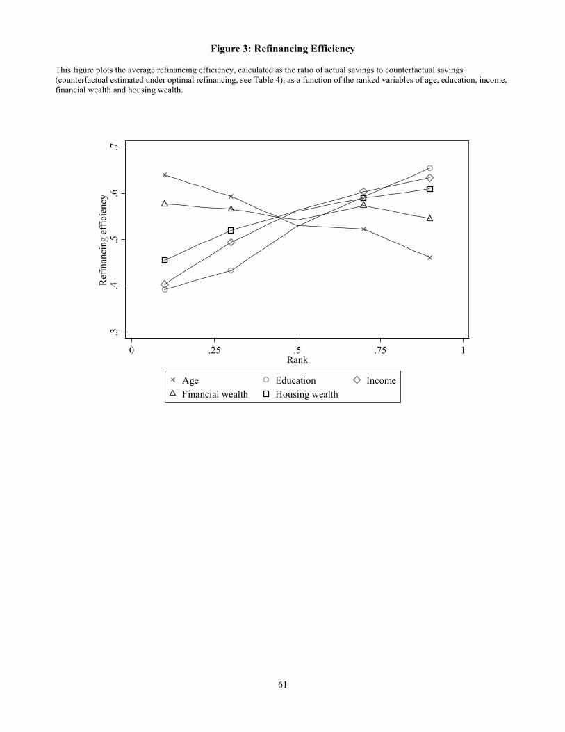
Figure 3 summarizes these patterns graphically. The figure plots refinancing effi ciency,

defined as the ratio of realized savings to optimal savings in DKK, across quintiles of the

distribution for age, education, income, financial wealth, and housing wealth. Refinancing

effi ciency declines with age from about 65% to about 45%, increases with education and

income from 40% to over 60% and with housing wealth from about 45% to 60%, and is

fairly flat just below 60% in relation to financial wealth. These estimates justify a concern

that the mortgage refinancing decision is challenging for some people. We now estimate a

structural refinancing model to gain greater insight about the nature of this challenge.

4 A Model of Slow Refinancing

4.1 A mixture model of refinancing behavior

A. State-dependent inaction: refinancing with psychological costs

Consider a model of mortgage choice in which the probability that a household i refinances

its fixed-rate mortgage at time t (the event yit = 1) depends on the household’s perceived

refinancing incentive, its responsiveness to the incentive, and a standard logistic distributed

stochastic choice error εit following Luce (1959).

The refinancing probability of the household i at time t can be written as

pi,t(yi,t = 1 | zit;ϕ, β) = p(exp(β)I∗(zit;ϕ) + εit > 0). (8)

Here zit is a set of household and mortgage characteristics at time t. The parameter vector

ϕ interacts with those characteristics to determine the level of the refinancing incentive I∗.

The parameter β governs the household’s responsiveness to the incentive; for simplicity we

do not allow this parameter to vary across households.

We model the refinancing incentive using the ADL model from the previous section, with

26

one important change. The refinancing cost κ(mit), which in the rational model depends

only on the size of the mortgage mit, is now replaced by

κ∗(mit,zit;ϕ) = κ(mit) + exp(ϕ′zit). (9)

Household characteristics can increase the perceived refinancing cost. The modified refi-

nancing incentive I∗(zit;ϕ) is given by equations (1)-(7), replacing (5) with (9).

This specification implies that the likelihood contribution of each household choice is:

Lit(ϕ, β) = Λ([2yi,t − 1][exp(β)I∗(zit;ϕ)]

), (10)

where Λ(.) is the inverse logistic function, Λ(x) = exp(x)/(1 + exp(x)). This model of

household choice underlies the commonly used logit regression.

B. Time-dependent inaction: a mixture model

To capture the phenomenon of time-dependent inaction, we use a mixture model.23 We

assume that households can be in one of two states h, which we call “awake”and “asleep”.

In each period a household is asleep with probability wit and awake with probability 1−wit,

where 0 < wit < 1. Awake households refinance with probability as given above in equation

(8). Asleep households refinance with zero probability, which can be captured numerically

by altering (8) to have a large negative refinancing incentive.

The probability that a household is asleep in any period is modeled by

wit(χ) =exp(χ′zit)

1 + exp(χ′zit). (11)

23Mixture models have a long history in statistics since Pearson (1894). A recent survey is presented inMcLachlan and Peel (2000). Two current applications where mixture models are used to uncover decisionrules are El-Gamal and Grether (1995) for Bayesian updating behavior, and Harrison and Rutström (2009)for models of decision-making under risk.

27

The likelihood contribution for household i is a finite mixture of proportions:

Lit(χ, ϕ, β) = wit(χ)Lasleepit (ϕ, β) + (1− wit(χ))Lawakeit (ϕ, β). (12)

This leads to the household log likelihood function over our sample specified as:

lnL(χ, ϕ, β) =∑t

∑i

ln (Lit(χ, ϕ, β)) . (13)

This framework models deviations from rational refinancing using two parameter vectors

χ and ϕ and a scalar parameter β. The parameter vector χ captures the demographic

determinants of the probability that a household is awake and responding to refinancing

incentives in a given period. The parameter vector ϕ determines whether particular de-

mographic characteristics are associated with a higher or lower psychological refinancing

cost. Finally, the parameter β determines the responsiveness of households to the modified

refinancing incentive. One interpretation of this parameter is that it reflects unobserved

household-level shocks to the refinancing threshold level, uncorrelated across households and

over time.

Intuitively, these parameters determine a set of curves like those illustrated in Figure 8

below. Each curve relates the refinancing frequency for a household with a given set of

demographic characteristics to the ADL refinancing incentive at a point in time. The model

implies that each curve has a logistic form, close to zero for highly negative incentives and

positive for highly positive incentives. The height of the curve for highly positive incentives

measures the probability that the given type of household is awake. The horizontal position

of the point where the curve reaches half this height measures the increment to the ADL

threshold implied by the psychological refinancing costs for this type of household. The

slope of the curve at this point is governed by the parameter β, which for simplicity we do

not allow to vary with household demographics.

Together, the model’s parameters tell us the relative importance of time-dependent and

28

state-dependent inaction in explaining failures to refinance. For example, if the parameters

ϕ are estimated to be zero, then there are no psychological costs of refinancing. In this

case every household will eventually refinance whenever they face a positive ADL incentive

to do so, implying that the problem is time-dependent inaction. If on the other hand the

parameters χ imply that households are always awake, then households will refinance when-

ever they reach the threshold determined by their particular psychological refinancing costs,

implying that state-dependent inaction is the cause of refinancing failures. In the former

case a modest decline in interest rates will eventually induce all households to refinance,

whereas in the latter case a sizeable interest rate movement is required for some households

to overcome the psychological costs that inhibit refinancing.

4.2 Estimating the model

A. Parameter estimates and their implications

Table 5 presents baseline estimates of the model laid out in the previous section. The

table reports, for each demographic characteristic, the elements of the parameter vectors χ

and ϕ corresponding to that characteristic. The model includes dummies for the current

quarter and the age of the mortgage, which are assumed to enter the vector χ but not the

other parameter vectors; in other words, time and mortgage age are allowed to affect the

probability of considering a refinancing but not the psychological costs of refinancing. The

table also reports the estimate of the parameter β.

To characterize the overall fit of this model, Table 5 reports a pseudo-R2 statistic of

8.3%, calculated from the log likelihood ratio between the estimated model and a simple

mixture model that includes only a constant probability that a household is awake. As

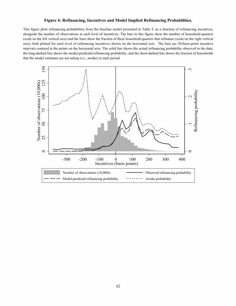
an alternative way to understand the ability of the model to fit the data, in Figure 4 we

show the sample distribution of incentives, together with the observed sample refinancing

probability at each incentive level. As previously discussed, most incentives are negative but

there is a substantial fraction of positive incentives. The observed refinancing probability

29

increases strongly around the zero level, peaking at an incentive slightly above 1%. Very few

observations have positive incentives greater than this, so the observed sample refinancing

probability at high incentive levels is based on limited data and is correspondingly noisy.

Figure 4 also shows our model’s predicted refinancing probability and the estimated av-

erage probability that households in each incentive bin are awake. The model-predicted

refinancing probability captures the overall cross-sectional pattern of refinancing quite well,

although it underpredicts refinancings with extremely negative incentives and overpredicts

refinancings with extremely positive incentives. The figure also shows that the probability

that households are awake is somewhat noisy across bins, but averages about 15% for house-

holds with negative or low positive incentives, and declines to below 10% for households

with high positive incentives. This pattern is the result of demographic variation in the

population at each incentive level, as incentives do not directly enter our specification for

the probability that households are awake.

We summarize the implications of our model estimates in a series of figures and in Table

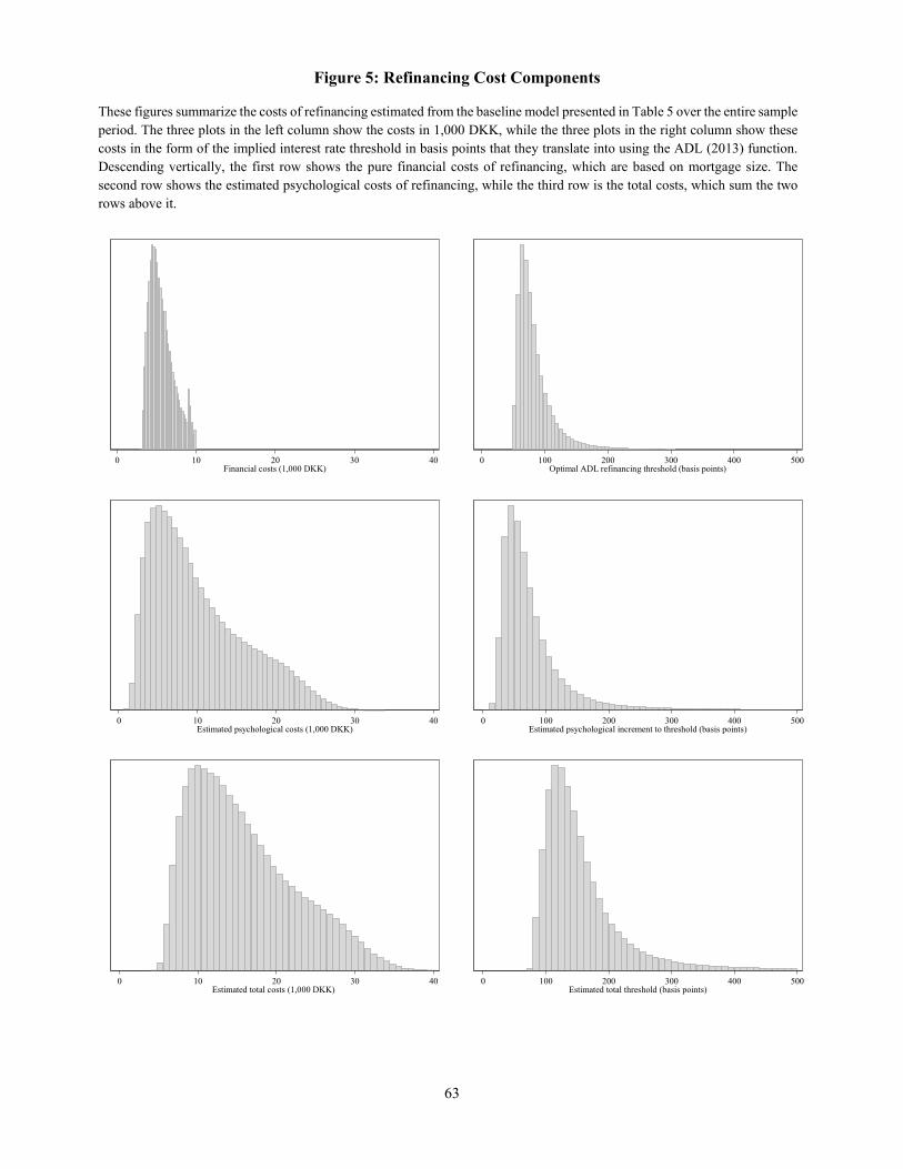
6. Figure 5 shows the estimated cross-sectional distribution of refinancing costs and their

implications for the interest savings that induces refinancing. The left side of the figure

measures refinancing costs in DKK, while the right side reports the implications of these

costs for the position of the interest threshold. The top left panel shows financial refinancing

costs varying from a little over DKK 3, 000 to the upper winsorization point just below DKK

10, 000, with a mean of DKK 5, 700. The top right panel reports the distribution of the

corresponding ADL refinancing threshold, varying from about 50 to about 250 basis points,

with a mean of 84 basis points and standard deviation of 30 basis points.

The middle left panel of Figure 5 shows the psychological refinancing costs in DKK,

varying from almost zero to about DKK 30, 000 with a mean just above DKK 10, 000.

Unsurprisingly, these costs lead to large increases in the threshold that triggers refinancing,

as shown in the middle right panel of Figure 5. Threshold increases have a mean that is

comparable to the ADL threshold, but a standard deviation that is more than 2 times greater

30

as reported in Table 6. Finally, the bottom panels of Figure 5 show the distributions of

total refinancing costs and the total threshold that triggers refinancing. The total threshold

is shifted to the right and spread out by the psychological refinancing costs, with a mean of

165 basis points and a standard deviation of 93 basis points.

A striking result in Table 6 is that households’ADL refinancing thresholds are almost

uncorrelated with their psychological refinancing costs in DKK, but are strongly positively

correlated with the increments to the refinancing threshold caused by those psychological

refinancing costs. The correlation between the ADL threshold and the psychological refi-

nancing cost is −0.02, but the correlation between the ADL threshold and the psychological

increment to the refinancing threshold is 0.87. The reason for this pattern is that refinancing

costs in DKK have a larger impact on the refinancing threshold for smaller, older mortgages.

Households with these mortgages therefore tend to have both higher ADL thresholds and

higher increases in the thresholds caused by their psychological refinancing costs.

Turning to time-dependent inaction, the top panel of Figure 6 reports the cross-sectional

distribution of the probability that households were asleep in a typical quarter of our sample

(using sample average time effects and mortgage age effects). There is strong time-variation

in this distribution as shown in the bottom panel of Figure 6 using a box-whisker plot.

Quarters with low refinancing activity are fit by the model using time fixed effects that

imply a high probability that all households are asleep in those quarters.24 Over the whole

sample, the average probability that a household is asleep is 0.83, with a standard deviation

of 0.13 (that includes both cross-sectional variation and variation over time for a given

household).

Cross-sectionally, there is a strong negative correlation between the probability that a

household is asleep and psychological refinancing costs measured in monetary units. The

24While time-variation in inaction is not the focus of our paper, we have verified using Google Trendsthat internet search activity for Danish refinancing terms moves closely with the refinancing rate (OnlineAppendix Figure B6) and inversely with the cross-sectional average probability that households are asleepin each quarter (Figure B7). It is also possible that social interactions, of the sort measured by Maturanaand Nickerson (2017), contribute to the time effect.

31

correlation is −0.69 in a typical quarter (using sample average time effects and mortgage age

effects for the asleep probability), as reported in the bottom panel of Table 6 and illustrated in

the top panel of Figure 7 using a scatter diagram. The reason, as we discuss in greater detail

below, is that younger households with higher socioeconomic status are more likely to be

awake but also have higher psychological refinancing costs in DKK. However, this correlation

disappears when we measure the psychological increment to the refinancing threshold. Table

6 reports a correlation of only −0.01 between the probability that a household is asleep and

the psychological threshold increment, a low correlation that is illustrated in the bottom

panel of Figure 7. The discrepancy arises because young households with high socioeconomic

status tend to have larger mortgages whose refinancing thresholds are less sensitive to the

level of refinancing costs in DKK.

The response coeffi cient β also has an important influence on the behavior of households

in the model. Figure 8 illustrates the response of an awake household to variation in the

refinancing incentive around zero (the point where the interest saving equals the modified

threshold). The logistic curve relating the incentive to the refinancing probability becomes

steeper as β increases, and for an infinite β would jump discontinuously from zero to one as

the incentive crosses zero. Our estimate of β implies that the refinancing probability moves

from about 25% to about 75% as the incentive moves from −50 to 50 basis points.

It is natural to ask whether the model estimated in Table 5 fits the data significantly

better than restricted models that exclude one or more of the effects we have discussed. In

Table 7 we address this issue by estimating a sequence of such restricted models, first setting

all demographic coeffi cients to zero and allowing only mortgage age and current quarter

effects on the asleep probability; then allowing free demographic effects on psychological

refinancing costs but none on the asleep probability; then free demographic effects on the

asleep probability but none on psychological refinancing costs; and finally imposing that

demographic effects on psychological refinancing costs and the asleep probability, as captured

by the coeffi cient vectors ϕ and χ, are proportional to one another. The importance of

allowing both types of demographic effects is indicated by the fact that all restricted models

32

are strongly rejected statistically, and the various restricted models achieve only about 2/3

of the improvement in pseudo-R2 statistics, over a model without demographic effects, that

is achieved by our full unrestricted model.

B. Cross-sectional variation in the determinants of slow refinancing

We now turn to a more detailed analysis of the mapping between Danish households’

demographic characteristics, their probability of considering a refinancing, and their psycho-

logical refinancing costs. Inspection of the coeffi cients on dummy variables in Table 5 shows

that some demographic characteristics are associated with faster refinancing through both

channels. Financial literacy of the household or the family has this effect, as do life events

such as getting married or having children. On the other hand, there are also characteristics

that move people closer to the rational benchmark in one dimension but further away in the

other. For example, married couples are more likely to consider a refinancing but have

higher psychological refinancing costs than unmarried couples, while immigrants have the

opposite pattern.

Table 5 also reports the coeffi cients on ranked variables: age, education, income, financial

wealth, and housing wealth. Previous literature has suggested that such variables may have

nonlinear effects. For example Agarwal, Driscoll, Gabaix, and Laibson (2009) report nonlin-

ear effects of age on many financial decisions, with financial sophistication increasing among

younger people as they gain experience, and decreasing among older people perhaps because

of cognitive decline. We have tried two different ways of allowing for such nonlinearities,

either using a piecewise linear function with a kink at the median (achieved by adding the

absolute value of the demeaned rank to the regression), or using a quadratic function (by

adding twice the squared demeaned rank, a normalization that allows direct comparison of

the coeffi cients in the two specifications). We have found qualitatively similar results with

either method and report the quadratic specification in the paper.

To understand the implied marginal effects of ranked variables, Figure 9 plots the vari-

ability in the estimated probability of being asleep, the estimated psychological costs of

33

refinancing in DKK, and the estimated psychological increment to the refinancing threshold,

as functions of the ranked variables. The figure is based on a two-step procedure in which the

full model is used to estimate refinancing probability, and then the fitted refinancing proba-

bility is regressed on the demographic variables, including dummy variables, but excluding

mortgage characteristics. This procedure implies that the effects of mortgage age and size

covariation with demographic characteristics are attributed to those characteristics, rather

than holding mortgage variables constant as demographic characteristics vary. It therefore

conveys a more accurate impression of how implied behavior varies cross-sectionally in our

model.

The top panel of Figure 9 shows that older households are more likely to be asleep, while

households with higher education, income, financial wealth, and housing wealth are all less

likely to be asleep. The middle panel of Figure 9 shows that middle-aged people have

higher psychological refinancing costs in DKK than younger or older people. Households

with higher education, income, financial wealth, and housing wealth all have somewhat

higher psychological refinancing costs, helping to explain the negative correlation between

the probability that a household is awake and the household’s psychological refinancing

costs measured in DKK that was illustrated in Figure 7. However, the bottom panel

of Figure 9 shows that the psychological increment to the refinancing threshold varies little

with education, income, and housing wealth and increases strongly only with financial wealth.

This is consistent with the fact that people with high financial wealth tend to have small

mortgages, controlling for their other characteristics, so their DKK refinancing costs have a

large impact on their refinancing threshold– while the opposite is true for people with high

education, income, and housing wealth. The hump-shaped pattern with age is preserved in

the bottom panel of Figure 9.

The results in Figure 9 suggest that some component of the psychological DKK refinanc-

ing costs estimated by our model may correspond to the value of time, which is plausibly

higher for middle-aged people and for people with higher income and wealth. This interpre-

tation might also explain the result shown in Table 5 that psychological DKK refinancing

34

costs are higher for families with children present. However, as we have discussed, the

pass-through of this effect to mortgage refinancing behavior is muted by the inherent re-

sponsiveness of households with large mortgages to the refinancing incentives generated by

low interest rates.

4.3 Robustness

In this section we verify that our results are not sensitive to our choice of mortgage sample,

to the parameterization of the ADL optimal refinancing model, or to our decision to use the

ADLmodel as our rational refinancing benchmark. We also compare the ADL threshold with

the recommendations of Danish financial advisers, and with the behavior of those Danish

households who refinance early in their cohort. Finally, we examine the robustness of our

results to the logistic functional form assumed in our stochastic choice model.

A. Alternative mortgage samples

Online Appendix C replicates Table 5 and Figures 4—7 and 9, excluding all cash-out and

maturity extension refinancing from our sample. Online Appendix D restricts the mortgage

sample to include only mortgages with principal value above DKK 250,000 and remaining

maturity of at least 20 years. These larger and longer-maturity mortgages have refinancing

thresholds that are less sensitive to parameter inputs and the choice of refinancing model.

In both these cases, our model delivers qualitatively similar results to those reported in the

paper.

B. Alternative parameter choices for the ADL model and behavioral refinancing model

We have explored the sensitivity of the ADL threshold to changes in the assumed parame-

ters. Online Appendix Figure E1 shows that a 50% reduction in the assumed interest-rate

volatility σ lowers the threshold by about 20 basis points on average, while Figure E2 shows

that a 50% reduction in the household’s discount rate ρ lowers it by less than 10 basis points.

These changes are small enough to have very little impact on our conclusions about house-

35

hold behavior. Unsurprisingly, when we replicate Table 5 and Figures 4—7 and 9 with these

two parameter modifications, in Online Appendices F and G, we obtain similar results to

those in the paper.

Online Appendix H assumes a constant mortgage termination probability of 10% for all

households, an input to the ADL model that affects the position of the optimal refinancing

threshold. Online Appendix I allows demographic characteristics to affect the parameter β

that governs household responsiveness to incentives. Results in these cases are again similar

to the base case. We have also considered a model in which households are more likely to

be awake when interest rates cross discrete “round number”thresholds, but have not found

any evidence of such effects.

C. Alternative model of optimal refinancing

In a more ambitious exercise, we recompute optimal refinancing thresholds using the

approach of Chen and Ling (CL 1989), which differs from the ADL approach in several

substantive ways.25 The CL model treats mortgages as having a finite maturity, with an

early prepayment that occurs (in the absence of refinancing) at a known future date. The

short-term interest rate is assumed to follow a geometric Brownian motion, and a term

structure model is used to derive the corresponding mortgage rate.

Most importantly, in the CL model refinancing can only occur once rather than multiple

times. Our application of the ADL model ignores the fact that under Danish rules, a refi-

nancing today reduces the value of future refinancing opportunities by increasing mortgage

principal; but the CL model makes future refinancing impossible, and so (setting aside other

differences between the two models), the difference between the CL and ADL thresholds

provides an upper bound on the magnitude of this effect.

25The ADL and CL models are similar in one important respect: they both assume that mortgage borrowersare risk-neutral with respect to refinancing proceeds. We are not aware of any threshold models that allowfor borrower risk aversion. Risk aversion would likely reduce the refinancing threshold (since refinancingtoday locks in an interest saving as opposed to waiting for a potentially larger but risky saving tomorrow),which would increase our estimates of psychological refinancing costs. However, if interest rates are positivelycorrelated with household income, it is possible that delaying refinancing would insure income risk, in whichcase risk aversion could increase the threshold and lower our estimates of psychological refinancing costs.

36

The CL model does not deliver an analytical formula for the optimal refinancing thresh-

old, so we use numerical simulations to derive thresholds corresponding to a large number of

mortgages with given parameters (including candidate psychological refinancing costs), and

interpolate thresholds for other mortgages.

Online Appendix J discusses the CL model and our implementation of it in greater

detail, and compares the CL and ADL refinancing thresholds in our sample. We find that

the average difference between the CL and ADL thresholds is 5 basis points, the median

difference is 1 basis point, the standard deviation of the difference is 41 basis points, and the

interquartile range runs from -15 basis points to 22 basis points. The CL and ADL thresholds

have a cross-sectional correlation of 0.75. Importantly, the differences between the two

thresholds are large only for mortgages with lower principal and shorter maturities; these

mortgages have high refinancing thresholds whose exact values are sensitive to assumptions,

but for this very reason they do not play an important role in our analysis because both the

CL and ADL models imply that they should not be refinanced.26

Online Appendix K replicates Table 5 and Figures 4—7 and 9 using CL thresholds in

place of ADL thresholds. Online Appendix L repeats this exercise for the smaller sample of

mortgages, already considered in Appendix D, that have principal value above DKK 250,000

and remaining maturity of at least 20 years. There are some shifts in the curves relating

ranked variables to psychological costs of refinancing measured in DKK, but no other changes

worthy of note.

D. Reconciliation with financial advice and prompt refinancing behavior

We complement the CL analysis with two further reality checks on the ADL refinancing

26Interestingly, among mortgages with high principal and long maturity, there is a region where thecorrelation between the ADL and CL thresholds is actually negative. This is because such mortgages differprimarily in their exogenous termination probability, which is modeled as a constant hazard by ADL andas a shift in a known future termination date by CL. A higher termination probability raises the ADLrefinancing threshold, but lowers the CL threshold by reducing the value of the option to wait for lowermortgage rates in the future. Appendix J discusses this phenomenon in greater detail. It does not affectour empirical results because both the ADL and CL thresholds for mortgages of this sort are small relativeto the thresholds that trigger household refinancing in our data.

37

threshold. First, we verify that the shape of the ADL threshold illustrated in Figure 1

is broadly consistent with the recommendations of Danish financial advisers. A typical

recommendation from the real estate advisory firm Bolius Boligejernes Videncenter (see

https://www.bolius.dk/omlaegning-af-dit-realkreditlaan-17799/) is to refinance when a) the

difference between the old and the new coupon is at least 150 basis points, b) the outstanding

principal is at least DKK 250,000, and c) the remaining time to maturity is at least 5 to

10 years. Mortgages with large outstanding principal and/or long remaining maturity are

recommended to refinance at a lower coupon differential. In our sample period the difference

between the yield and the coupon on new mortgages is on average 36 basis points, implying

from condition a) that refinancing is advantageous when the difference between the old

coupon and the new yield is 114 basis points. In comparison the median household in our

sample has an ADL threshold of 75 basis points. While this is 39 basis points lower, we note

that the average mortgage in our sample has greater outstanding principal (DKK 926,000)

and a longer time to maturity (23 years) than the mortgage contemplated by Bolius.

Second, we check the relationship between the empirically measured incentives of prompt

refinancers and the ADL threshold. To ensure that we pick up individuals who respond

promptly to incentives, we conduct this exercise for loans issued in the last quarter of 2009

or later. We do so to avoid misclassifying sluggish households from early loan cohorts as

prompt refinancers during our sample period.

For each cohort of issued loans, we define individuals as prompt refinancers if they are

in the first few percent of households to refinance in a given loan cohort. We vary this

percentage cutoff, picking the first 2.5%, 5%, and 10% of households to refinance. We

measure the average incentive for each such household, the interest saving relative to the

ADL threshold, in the first quarter in the time series in which the percentage cutoff is hit.

An example might make this easier to understand. The first loan cohort that we consider

has an issue date of 2009Q4 and contains 7,554 loans. In this cohort, 47 loans refinance in

2010Q1, 73 in 2010Q2, 398 in 2010Q3, 503 in 2010Q4, and so on. The first quarter in which

38

the 5% cutoff for prompt refinancing is exceeded is 2010Q3, in which 5.2% of all loans in the

2009Q4 cohort are refinanced. Thus, households in the 2009Q4 cohort who refinanced their

mortgages in 2010Q3 are classified as “prompt”refinancers, and we calculate their average

incentives in that quarter to be 8 basis points.

When we average across loan cohorts using weights proportional to the number of loans

issued in each cohort, we find that prompt refinancers classified with a 2.5% cutoff have a

weighted average incentive of 6 bp; the 5% cutoff yields 29 bp, and a 10% cutoff, 38 bp.

This simple exercise produces average incentives for prompt refinancers that appear to be

close to zero, which is consistent with the ADL formula approximately capturing the rational

refinancing threshold in the Danish institutional setting. Online Appendix M provides more

details about this exercise.

E. Functional form of the stochastic choice model

Finally, we explore the effect of functional form misspecification on our parameter es-

timates. Online Appendix N uses a probability distortion, analogous to that used in be-

havioral finance models, to alter the assumed logistic distribution of the stochastic choice

error. We estimate our model on data simulated from the misspecified model. We find that

symmetric probability distortion has minimal effect on any of the parameters of our model,

while an asymmetric distortion is picked up by our estimation procedure as an increase in

the true unconditional probability that households are asleep and the unconditional average

psychological refinancing cost. However, in no case does functional form misspecification

have any major effect on the parameter estimates that capture cross-sectional variation in

time-dependent and state-dependent inaction, which are the main concern of our paper.

4.4 Applying the model

In this section we use our model to explore the effects on refinancing of various plausible

alterations to the mortgage system in a hypothetical simulation. We consider a random

39

sample of mortgage borrowers drawn from the Danish population at the start of our refi-

nancing sample period in the first quarter of 2010. We lower the interest rate from the actual

level by 172 basis points, a decline chosen to give 90% of the sample positive refinancing

incentives relative to the ADL threshold. We fix the interest rate at this low level for three

years, and track refinancing behavior over time in various alternative scenarios.

As a first exercise, we illustrate the effects of different components of our model on

aggregate refinancing rates and the refinancing effi ciency of different types of borrowers. The

top panel of Figure 10 shows cumulative aggregate refinancing rates in a fully rational model

with automatic refinancing at the ADL threshold (labeled AM), a pure state-dependent

model with rational refinancing at the threshold augmented by our estimated psychological

refinancing costs, a pure time-dependent model in which information-gathering costs lead to

rational refinancing at the ADL threshold only by households that are awake, and finally

our full model with all components including a smooth refinancing response to incentives.

Unsurprisingly the cumulative refinancing rate for the fully rational model reaches 90% in

the first quarter and stays there, while the cumulative refinancing rate in the state-dependent

model with augmented thresholds is lower at just above 60% but has the same time pattern.

A pure time-dependent model has a smoothly rising cumulative refinancing rate, and our

full model has the same time pattern at a lower level.

The second and third panels of Figure 10 show the refinancing rates of different groups of

borrowers as a fraction of the rational refinancing rates for the same groups. This is closely

related to the measure of refinancing effi ciency illustrated in Figure 3, although for simplicity

we do not calculate interest savings. We illustrate these refinancing effi ciency measures for

borrowers ranked by age in the second panel, and by income in the third panel. The measures

can be calculated at any period of the simulation, and we choose to report results two years

after the initial interest rate decline. The second panel shows that psychological refinancing

costs lower the refinancing effi ciency of middle-aged households relative to younger and

older households, while information-gathering costs lower the refinancing effi ciency of older

households. In our full model the latter effect dominates, just as we saw in the data.

40

The third panel shows that psychological refinancing costs lower the refinancing effi ciency of

higher-income households, while information-gathering costs lower the refinancing effi ciency

of poorer households which is the dominant effect in both the simulation and the data.

In Figure 11 we repeat the above analysis for three modifications of the Danish mort-

gage system designed specifically to improve the refinancing effi ciency of older and poorer

households. The first modification (labeled R) rebates the fixed component of the mort-

gage refinancing fee (DKK 3, 000) and removes the caps on the fees to make the mortgage

refinancing fee proportional. This eliminates the tendency of smaller mortgages (which are

disproportionately held by older and poorer households) to have higher ADL thresholds.

The second modification advertises refinancing opportunities (lowers information-gathering

costs) in such a way that one-half of all households who were asleep are woken up. The third

modification combines these two policies. The top panel of Figure 11 shows that waking

households up is a much more powerful way to increase aggregate refinancing rates. This

may not be surprising given the large size of the interest rate reduction we are consider-

ing, which is suffi cient to give 90% of households an incentive to refinance relative to the

ADL threshold. The second and third panels similarly show that waking households up is

the best way to improve the refinancing effi ciency of older and poorer households, although

refinancing rebates do have a larger effect on poorer households as one would expect.

These findings are relevant for the literature on the mortgage refinancing channel of mon-

etary transmission (Auclert 2016, Agarwal et al. 2015, Beraja et al. 2017, Di Maggio et al.

2016). Expansionary monetary policy stimulates the economy in part by lowering mortgage

rates, which in turn increases household consumption. However, in a fixed-rate mortgage

system lower mortgage rates relieve the budgets only of households that refinance their mort-

gages. Such budget relief is persistent, and therefore should stimulate consumption roughly

one-for-one for households that have either no binding borrowing constraints (permanent

income consumers) or fixed and binding borrowing constraints. To the extent that budget

relief relaxes borrowing constraints by permitting households to extract home equity, or to

increase uncollateralized borrowing, the effect on consumption may initially exceed the ef-

41

fect on budget relief. Refinancing failures by poorer households limit the passthrough from

declining mortgage rates to consumption, and particularly do so to the extent that poorer

households are more likely to face borrowing constraints that can be relaxed by budget re-

lief. Policies to mitigate such refinancing failures– by reducing information-gathering costs

or even refinancing mortgages automatically– therefore have the potential to increase the

effectiveness of monetary policy stimulus during economic downturns.

5 Conclusion

In this paper we have documented slow mortgage refinancing behavior among Danish house-

holds. The Danish context is particularly advantageous for studying this type of household

behavior because the Danish mortgage system places no restrictions on refinancing that does

not involve cash-out, so households that pass up opportunities to substantially reduce their

mortgage costs are not constrained, but are making mistakes in managing their finances. In

addition, the Danish statistical system allows us to measure the demographic and economic

characteristics of households in great detail.

We distinguish between time-dependent and state-dependent models of slow refinancing.

A time-dependent model has a reduced probability of refinancing at any incentive, while a

state-dependent model increases the threshold that triggers refinancing, equivalent to the

addition of psychological costs to the direct financial costs of refinancing. We find that older

households and those with lower education, income, housing wealth, and financial wealth

are all well described by a time-dependent model, whereas psychological costs of refinancing

are greatest for middle-aged households and those with high financial wealth. The cross-

sectional variation in psychological refinancing costs is consistent with the view that these

costs may in part capture the high value of time for certain households. Time-dependent slow

refinancing is the primary reason why older households and those with lower socioeconomic

status achieved low interest savings from refinancing during our sample period, relative to

42

the savings achievable with an optimal refinancing strategy.

Both our methodology and our findings have relevance beyond the context of this pa-

per. We believe that the mixture model we have used to estimate time-dependent slow

refinancing is a promising econometric method for estimating the prevalence of behavioral

biases in the population, and a useful alternative to the competing-risks proportional hazard

framework of Deng, Quigley, and Van Order (2000) for modeling heterogeneous prepayment

behavior. Our findings reinforce concerns that financial capabilities deteriorate late in life

(Agarwal, Driscoll, Gabaix, and Laibson 2009) and that poorer households make worse finan-

cial decisions (Campbell 2006, Calvet, Campbell, and Sodini 2009b, Badarinza, Campbell,

and Ramadorai 2016), contributing to inequality of wealth (Piketty 2014, Bach, Calvet, and

Sodini 2015, Campbell 2016). Finally, our results imply that the effect of expansionary

monetary policy on household consumption is weakened in economies with predominantly

fixed-rate mortgages, not only by barriers to refinancing that may result from low credit

scores and house prices, as emphasized by Agarwal et al. (2015), Beraja et al. (2017), and

Di Maggio et al. (2016), but also by the slow reaction of many households to refinancing

opportunities.

43

References

Abel, Andrew B., Janice C. Eberly, and Stavros Panageas, 2007, “Optimal Inattention tothe Stock Market”, American Economic Review: Papers and Proceedings 97, 244—249.

Abel, Andrew B., Janice C. Eberly, and Stavros Panageas, 2013, “Optimal Inattention tothe Stock Market with Information Costs and Transactions Costs”, Econometrica 81,1455—1481.

Agarwal, Sumit, Gene Amromin, Souphala Chomsisengphet, Tomasz Piskorski, Amit Seru,and Vincent Yao, 2015, “Mortgage Refinancing, Consumer Spending and Competition:Evidence from the Home Affordable Refinancing Program”, NBER Working Paper21512.

Agarwal, Sumit, John Driscoll, and David Laibson, 2013, “Optimal Mortgage Refinancing:A Closed Form Solution”, Journal of Money, Credit, and Banking 45, 591—622.

Agarwal, Sumit, John Driscoll, Xavier Gabaix, and David Laibson, 2009, “The Age ofReason: Financial Decisions Over the Life Cycle and Implications for Regulation”,Brookings Papers on Economic Activity 2, 51—101.

Agarwal, Sumit, Richard J. Rosen, and Vincent Yao, 2016, “Why Do Borrowers MakeMortgage Refinancing Mistakes?”, Management Science 62, 3494—3509.

Agnew, Julie, Pierluigi Balduzzi, and Annika Sunden, 2003, “Portfolio Choice and Tradingin a Large 401(k) Plan”, American Economic Review 93, 193—215.

Alvarez, Fernando, Luigi Guiso, and Francesco Lippi, 2012, “Durable Consumption andAsset Management with Transaction and Observation Costs”, American EconomicReview 102, 2272—2300.

Alvarez, Fernando, Francesco Lippi, and Luigi Paciello, 2011, “Optimal Price Setting WithObservation and Menu Costs”, Quarterly Journal of Economics 126, 1909—1960.

Anagol, Santosh, Vimal Balasubramaniam, and Tarun Ramadorai, 2018, “Endowment Ef-fects in the Field: Evidence from India’s IPO Lotteries”, forthcoming Review of Eco-nomic Studies.

Andersen, Steffen, John Y. Campbell, Kasper Meisner Nielsen, and Tarun Ramadorai,2018, “Appendix to Inattention and Inertia in Household Finance”, available online atauthors’websites.

Archer, Wayne R., David C. Ling, and Gary A. McGill, 1996, “The Effect of Income andCollateral Constraints on Residential Mortgage Terminations”, Regional Science andUrban Economics 26, 235—261.

44

Auclert, Adrien, 2016, “Monetary Policy and the Redistribution Channel”, unpublishedpaper, Stanford University.

Bach, Laurent, Laurent E. Calvet, and Paolo Sodini, 2015, “Rich Pickings? Risk, Return,and Skill in the Portfolios of the Wealthy”, unpublished paper, Swedish House ofFinance, EDHEC Business School, and Stockholm School of Economics.

Badarinza, Cristian, John Y. Campbell, and Tarun Ramadorai, 2016, “International Com-parative Household Finance”, Annual Review of Economics 8, 111—144.

Badarinza, Cristian, John Y. Campbell, and Tarun Ramadorai, 2017, “What Calls toARMs? International Evidence on Interest Rates and the Choice of Adjustable RateMortgages,”forthcoming Management Science.

Bajo, Emanuele and Massimiliano Barbi, 2016, “Out of Sight, Out of Mind: Media Cover-age, Financial Literacy, and Mortgage Refinancing”, unpublished paper, University ofBologna.

Bennett, Paul, Richard Peach, and Stavros Peristiani, 2001, “Structural Change in theMortgage Market and the Propensity to Refinance”, Journal of Money, Credit, andBanking 33, 955—975.

Beraja, Martin, Andreas Fuster, Erik Hurst, and Joseph Vavra, 2017, “Regional Hetero-geneity and Monetary Policy”, NBER Working Paper 23270.

Bhutta, Neil and Benjamin J. Keys, 2016, “Interest Rates and Equity Extraction Duringthe Housing Boom”, American Economic Review 106, 1742—1774.

Bilias, Yannis, Dimitris Georgarakos, and Michael Haliassos, 2010, “Portfolio Inertia andStock Market Fluctuations”, Journal of Money, Credit and Banking 42, 715—742.

Brueckner, Jan K. and James R. Follain, 1988, “The Rise and Fall of the ARM: An Econo-metric Analysis of Mortgage Choice,”Review of Economics and Statistics 70, 93—102.

Brunnermeier, Markus K. and Stefan Nagel, 2008, “DoWealth Fluctuations Generate Time-Varying Risk Aversion? Micro-Evidence on Individuals”, American Economic Review98, 713—736.

Bucks, Brian and Karen Pence, 2008, “Do Borrowers Know Their Mortgage Terms?”, Jour-nal of Urban Economics 64, 218—233.

Caballero, Ricardo J. and Eduardo M. Engel, 1991, “Dynamic (S,s) Economics”, Econo-metrica 59, 1659—1686.

Calvet, Laurent, John Y. Campbell, and Paolo Sodini, 2009a, “Fight or Flight? PortfolioRebalancing by Individual Investors”, Quarterly Journal of Economics 124, 301—348.

45

Calvet, Laurent, John Y. Campbell, and Paolo Sodini, 2009b, “Measuring the FinancialSophistication of Households”, American Economic Review Papers and Proceedings 99,393—398.

Calvo, Guillermo A., 1983, “Staggered Prices in a Utility-Maximizing Framework”, Journalof Monetary Economics 12, 383—398.

Campbell, John Y., 2006, “Household Finance”, Journal of Finance 61, 1553—1604.

Campbell, John Y., 2013, “Mortgage Market Design”, Review of Finance 17, 1—33.

Campbell, John Y., 2016, “Restoring Rational Choice: The Challenge of Consumer Finan-cial Regulation”, American Economic Review: Papers and Proceedings 106(5):1—30.

Campbell, John Y. and Joao Cocco, 2003, “Household Risk Management and OptimalMortgage Choice”, Quarterly Journal of Economics 118, 1449—1494.

Campbell, John Y. and Joao Cocco, 2015, “A Model of Mortgage Default”, Journal ofFinance 70, 1495—1554.

Caplin, Andrew, 2016, “Measuring and Modeling Attention”, Annual Review of Economics8, 379—403.

Caplin, Andrew, Charles Freeman, and Joseph Tracy, 1997, “Collateral Damage: Refinanc-ing Constraints and Regional Recessions”, Journal of Money, Credit, and Banking 29,496—516.

Caplin, Andrew and John Leahy, 1991, “State-Dependent Pricing and the Dynamics ofMoney and Output”, Quarterly Journal of Economics 106, 683—708.

Caplin, Andrew and Daniel F. Spulber, 1987, “Menu Costs and the Neutrality of Money”,Quarterly Journal of Economics 102, 703—725.

Chen, Andrew and David Ling, 1989, “Optimal Mortgage Refinancing with StochasticInterest Rates”, AREUEA Journal 17, 278—99.

Chen, Hui, Michael Michaux, and Nikolai Roussanov, 2013, “Houses as ATMs? MortgageRefinancing and Macroeconomic Uncertainty”, unpublished paper, MIT, USC, andUniversity of Pennsylvania.

Choi, James J., David Laibson, Brigitte Madrian, and Andrew Metrick, 2002, “DefinedContribution Pensions: Plan Rules, Participant Decisions, and the Path of Least Re-sistance”, in James Poterba ed. Tax Policy and the Economy 16, 67—113.

Choi, James J., David Laibson, Brigitte Madrian, and Andrew Metrick, 2004, “For Bet-ter or for Worse: Default Effects and 401(k) Savings Behavior”, in David Wise ed.Perspectives on the Economics of Aging, University of Chicago Press.

46

DellaVigna, Stefano, and Joshua M. Pollet, 2007, “Demographics and Industry Returns”,American Economic Review 97, 1667—1702.

Deng, Yongheng and John M. Quigley, 2012, “Woodhead Behavior and the Pricing of Res-idential Mortgages”, unpublished paper, National University of Singapore and Univer-sity of California Berkeley.

Deng, Yongheng, John M. Quigley and Robert Van Order, 2000, “Mortgage Terminations,Heterogeneity, and the Exercise of Mortgage Options”, Econometrica 68, 275—307.

Dhillon, Upinder S., James D. Shilling, and C.F. Sirmans, 1987, “Choosing Between Fixedand Adjustable Rate Mortgages: Note”, Journal of Money, Credit, and Banking 19,260—267.

Di Maggio, Marco, Amir Kermani, Benjamin Keys, Tomasz Piskorski, Rodney Ramcha-ran, Amit Seru, and Vincent Yao, 2016, “Monetary Policy Pass-Through: MortgageRates, Household Consumption and Voluntary Deleveraging”, forthcoming AmericanEconomic Review.

Duffi e, Darrell, and Tong-sheng Sun, 1990, “Transactions Costs and Portfolio Choice in aDiscrete-Continuous-Time Setting”, Journal of Economic Dynamics and Control 14,35—51.

El-Gamal, Mahmoud A. and David M. Grether, 1995, “Are People Bayesian? UncoveringBehavioral Strategies”, Journal of the American Statistical Association 90, 1137—1145.

Gabaix, Xavier, Arvind Krishnamurthy, and Olivier Vigneron, 2007, “Limits of Arbitrage:Theory and Evidence from the Mortgage-Backed Securities Market”, Journal of Fi-nance 62, 557—595.

Gabaix, Xavier and David I. Laibson, 2002, “The 6D Bias and the Equity-Premium Puzzle,”in Ben S. Bernanke and Kenneth S. Rogoff eds. NBER Macroeconomics Annual 2001,MIT Press, Cambridge, MA, 257—312.

Gyntelberg, J., Kjeldsen, K., Baekmand Nielsen, M., and Persson, M., 2012, “The 2008Financial Crisis and the Danish Mortgage Market”, in A. Bardhan, R.H. Edelstein,and C.A. Kroll eds. Global Housing Markets: Crises, Policies, and Institutions, JohnWiley, 53—68.

Hall, Arden, 2000, “Controlling for Burnout in Estimating Mortgage Prepayment Models”,Journal of Housing Economics 9, 215—232.

Johnson, Kathleen W. and Geng Li, 2014, “Are Adjustable-Rate Mortgage Borrowers Bor-rowing Constrained?,”Real Estate Economics 42, 457—471.

Harrison, GlennW. and E. Elisabet Rutström, 2009, “Expected Utility Theory and ProspectTheory: One Wedding and a Decent Funeral,”Experimental Economics 12, 133—158.

47

Johnson, Eric, Stephan Meier, and Olivier Toubia, 2015, “Leaving Money on the KitchenTable: Exploring Sluggish Mortgage Refinancing Using Administrative Data, Surveys,and Field Experiments”, unpublished paper, Columbia Business School.

Kang, Pan and Stavros A. Zenios, 1992, “Complete Prepayment Models for MBS”, Man-agement Science 38, 1665—1685.

Keys, Benjamin J., Devin G. Pope, and Jaren C. Pope, 2016, “Failure to Refinance”,Journal of Financial Economics 122, 482—499.

Khandani, Amir E., Andrew W. Lo, and Robert C. Merton, 2013, “Systemic Risk and theRefinancing Ratchet Effect”, Journal of Financial Economics 108, 29—45.

Koijen, Ralph S.J., Van Hemert, Otto and Stijn Van Nieuwerburgh, 2009, “Mortgage Tim-ing,”Journal of Financial Economics 93, 292—324.

LaCour-Little, Michael, 1999, “Another Look at the Role of Borrower Characteristics inPredicting Mortgage Prepayments”, Journal of Housing Research 10, 45—60.

Laibson, David, 1997, “Golden Eggs and Hyperbolic Discounting”, Quarterly Journal ofEconomics 112, 443—478.

Lea, M., 2011, “Alternative Forms of Mortgage Finance: What Can We Learn from OtherCountries?”in N. Retsinas and E. Belsky eds., Moving Forward: The Future of Con-sumer Credit and Mortgage Finance, Joint Center for Housing Studies, Harvard Uni-versity, Cambridge, MA, and Brookings Institution Press, Washington, DC, 118—149.

Luce, R. Duncan, 1959, Individual Choice Behavior: A Theoretical Analysis, Wiley, NewYork, NY.

Madrian, Brigitte and Dennis Shea, 2001, “The Power of Suggestion: Inertia in 401(k)Participation and Savings Behavior”, Quarterly Journal of Economics 66, 1149—1188.

Matejka, Filip and Alisdair McKay, 2015, “Rational Inattention to Discrete Choices: ANew Foundation for the Multinomial Logit Model”, American Economic Review 105,272—298.

Maturana, Gonzalo and Jordan Nickerson, 2017, “Teachers Teaching Teachers: The Role ofNetworks on Financial Decisions”, unpublished paper, Emory University and BostonCollege.

McConnell, John J., and Manoj Singh, 1994, “Rational Prepayments and the Valuation ofCollateralized Mortgage Obligations”, Journal of Finance 49, 891—921.

McLachlan, Geoffrey and David Peel, 2000, Finite mixture models, Wiley, New York, NY.

Miles, David, 2004, The UK Mortgage Market: Taking a Longer-term View, HM Treasury,London, UK.

48

Moscarini, Giuseppe, 2004, “Limited Information Capacity as a Source of Inertia”, Journalof Economic Dynamics and Control 28, 2003—2035.

O’Donoghue, Ted, and Matthew Rabin, 1999, “Doing it Now or Later”, American EconomicReview 89, 103—124.

Pearson, Karl, 1894, “Contributions to the Mathematical Theory of Evolution”, Philosoph-ical Transactions of the Royal Society of London A, 71—110.

Piketty, Thomas, 2014, Capital in the 21st Century, Harvard University Press, Cambridge,MA.

Reis, Ricardo, 2006a, “Inattentive Consumers”, Journal of Monetary Economics 53, 1761—1800.

Reis, Ricardo, 2006b, “Inattentive Producers”, Review of Economic Studies 73, 793—821.

Schwartz, Allie, 2006, “Household Refinancing Behavior in Fixed-Rate Mortgages”, unpub-lished paper, Harvard University.

Schwartz, Eduardo S., and Walter N. Torous, 1989, “Prepayment and the Valuation ofMortgage-Backed Securities”, Journal of Finance 44, 375—392.

Sims, Christopher A., 2003, “Implications of Rational Inattention”, Journal of MonetaryEconomics 50, 665—690.

Stanton, Richard, 1995, “Rational Prepayment and the Valuation of Mortgage-Backed Se-curities”, Review of Financial Studies 8, 677—708.

Taylor, John B., 1980, “Aggregate Dynamics and Staggered Contracts”, Journal of PoliticalEconomy 88, 1—23.

Tracy, Joseph and Joshua Wright, 2012, “Payment Changes and Default Risk: The Impactof Refinancing on Expected Credit Losses”, Federal Reserve Bank of New York StaffReport No. 562.

Veldkamp, Laura, 2011, Information Choice in Macroeconomics and Finance, PrincetonUniversity Press, Princeton, NJ.

Veronesi, Pietro, 2010, Fixed Income Securities: Valuation, Risk, and Risk Management,John Wiley & Sons, Hoboken, NJ.

Woodford, Michael, 2009, “Information-Constrained State-Dependent Pricing”, Journal ofMonetary Economics 56, Supplement, S100—S124.

Woodward, Susan E., and Robert E. Hall, 2010, “Consumer Confusion in the MortgageMarket: Evidence of Less Than a Perfectly Transparent and Competitive Market”,American Economic Review 100, 511—515.

49

Woodward, Susan E. and Robert E. Hall, 2012, “Diagnosing Consumer Confusion andSub-Optimal Shopping Effort: Theory and Mortgage Market Evidence”, AmericanEconomic Review 102, 3249—3276.

Zandi, Mark and Cristian deRitis, 2011, “Improved HARPWill Expand Refinancing, BoostRecovery”, unpublished report, Moody’s Analytics.

Zhu, Jun, 2012, “Refinance and Mortgage Default: An Empirical Analysis of the HARP’sImpact on Default Rates”, unpublished paper, Freddie Mac.

50

51  

Table 1: Characteristics of Danish Fixed Rate Mortgages

These statistics are calculated using mortgages taken by all households in Denmark with an unchanging number of members, and with a single fixed rate mortgage at the beginning of each of the years listed in the columns. The final column shows the statistics for all unique mortgages in the full sample. The rows show, in order, the number of observations at the beginning of each year; the fraction refinancing by the end of the year (i.e., the fraction of households that refinanced their pre-existing mortgage voluntarily rather than refinancing for exogenous reasons such as moving house); the fraction refinancing by the end of the year to fixed rate mortgages (FRM); the average principal remaining on these mortgages in millions of Danish Kroner (DKK), i.e., the outstanding principal; the average number of years remaining before mortgages mature; and the average loan-to-value (LTV) ratio on these mortgages, calculated by the issuing mortgage banks. 2010 2011 2012 2013 2014 Total Initial # of observations 330,563 297,573 277,462 274,553 264,858 1,444,973 Fraction refinancing 0.226 0.086 0.253 0.156 0.193 0.171 FRM to FRM refinancing  0.429 0.342 0.692 0.769 0.849 0.617 Principal remaining (million DKK) 0.907 0.909 0.910 0.950 0.961 0.926 Years remaining on mortgage 23.382 22.923 22.498 23.031 22.828 22.951 Loan-to-value (LTV) ratio 0.569 0.547 0.604 0.624 0.638 0.594

   

52  

Table 2: Differences in Household Characteristics: Refinancing and Non-Refinancing Households

The first column shows the average of each of the characteristics reported in the rows, pooled across the entire sample from 2010-2014. Columns 2 to 7 report the difference of means between refinancing and non-refinancing households, with a negative value indicating a lower mean for refinancing households. Differences are reported either unconditionally across the entire sample (Column “All”), or conditional on the sub-periods in the column headers. In the rows, “single” households (male or female) have only one adult living at the address, and represent ~13% of the entire sample. “Married” households have two legally bound adults (including registered partnership of same-sex couples). “Children in family” takes the value of one if there are children in the household. “Immigrant” takes the value of one if there is an immigrant in the household. “No educational information” indicates an absence of data on this attribute. “Financially literate” takes the value of one if a member of the household has a degree in finance, or has had professional financial industry training. “Family financially literate” indicates when (non-household-resident) parents, siblings, in-laws, or children of the household are financially literate. “Getting married” refers to that change in marital status over the sample period. “Having children” indicates that households had a child within the last 12 months. “Rank of age” uses the age of the oldest person living in the household. “Rank of education” uses the best educated individual in the household. “Rank of income (financial wealth, housing assets)” uses the total income (financial wealth, housing assets) of the household. All ranks are computed each year across all households in the sample, and are normalized such that they take values between -0.5 and 0.5. ***, **, and * indicate coefficients that are significant at the one, five, and ten percent level by standard t-tests, respectively.

Difference between Refinancing and Non-Refinancing Households Average All*** 2010*** 2011*** 2012*** 2013*** 2014***

Single male household 0.130 -0.034*** -0.035*** -0.030*** -0.038*** -0.023*** -0.037*** Single female household 0.125 -0.024*** -0.030*** -0.026*** -0.022*** -0.013*** -0.027*** Married household 0.629 0.035*** 0.017*** 0.027*** 0.040*** 0.043*** 0.052*** Children in family 0.402 0.082*** 0.111*** 0.079*** 0.080*** 0.037*** 0.081*** Immigrant 0.077 -0.001*** 0.001*** -0.001*** 0.002*** 0.006*** 0.002*** No educational information 0.007 -0.003*** -0.003*** -0.012*** -0.002*** 0.016*** -0.003*** Financially literate 0.046 0.011*** 0.005*** 0.011*** 0.014*** 0.033*** 0.020*** Family financially literate 0.133 0.026*** 0.018*** 0.021*** 0.030*** -0.019*** 0.035*** Getting married 0.010 0.005*** 0.010*** 0.003*** 0.005*** -0.001*** 0.001*** Having children 0.043 0.020*** 0.034*** 0.025*** 0.018*** 0.004*** 0.009*** Rank of age 0.000 -0.061*** -0.106*** -0.067*** -0.006*** -0.003*** -0.046*** Rank of education 0.003 0.039*** 0.031*** 0.024*** 0.000*** 0.047*** 0.046*** Rank of income 0.002 0.059*** 0.061*** 0.049*** 0.027*** 0.051*** 0.069*** Rank of financial wealth -0.001 -0.055*** -0.101*** -0.076*** -0.100*** -0.004*** -0.027*** Rank of housing value 0.000 0.048*** 0.027*** 0.028*** 0.011*** 0.087*** 0.058*** Region North Jutland 0.125 0.000*** 0.004*** -0.007*** -0.006*** -0.042*** 0.025*** Region Middle Jutland 0.238 0.018*** 0.024*** 0.018*** 0.019*** 0.002*** 0.023*** Region Southern Denmark 0.228 -0.009*** -0.005*** 0.018*** -0.015*** 0.032*** 0.011*** Region Zealand 0.186 -0.021*** -0.013*** -0.023*** -0.019*** -0.003*** 0.009*** Region Copenhagen 0.222 0.014*** -0.010*** -0.003*** 0.021*** 0.078*** 0.026*** # of observations 5,648,323 ***5,648,323*** 1,224,654*** 1,245,845*** 1,178,468*** 1,075,044*** 1,093,582***

53  

Table 3: Errors of Commission and Omission

This table shows the incidence of errors of commission and omission, and the characteristics of households who commit errors of commission (refinancing when it is suboptimal), and errors of omission (not refinancing when it is optimal). We calculate the levels of incentives to engage in refinancing using the interest rate spread between the old and new mortgages less a spread computed using the Agarwal et al. (2013) formula which quantifies the option-value of waiting. We use these computed incentives, plus cutoff levels to control for possible noise in estimation, to identify errors of commission and omission. These cutoff levels are listed in the column headers, and work as follows: at a cutoff level of 0 (0.25), the interest rate spread is exactly equal to the computed Agarwal et al. (2013) threshold level (exceeds the Agarwal et al. (2013) threshold level by 25 basis points). In the rows below each column listing a cutoff value (ranging from 0 to 2 percentage points), we document the number of observations for which incentives plus cutoff are less than zero, and then assess the number of these observations for which households refinance. We then eliminate observations with maturity extension or cash-out refinancing to arrive at the number of observations classified as errors of commission, i.e., those who refinance despite incentives to do so being negative. Analogously, errors of omission are listed in the last block of figures as household-quarters in which there is no refinancing despite incentives less the cutoff being greater than zero.

Level of Cutoff 0 0.25 0.5 0.75 1 1.5 2 # Observations (incentives+cutoff<0) 3,334,598 2,451,889 1,887,602 1,306,298 734,150 228,936 89,297 # Observations, refinancing 57,974 33,885 24,370 12,701 5,934 2,142 891 # Observations, cash out or extend maturity 22,182 14,174 10,401 7,090 3,897 1,503 783 # Observations, errors of commission 35,792 19,711 13,969 5,611 2,037 639 108 Fraction with error of commission 0.011 0.008 0.007 0.004 0.003 0.003 0.001

# Observations (incentives-cutoff>=0) 2,313,725 1,573,255 1,092,938 796,624 524,195 228,739 104,944 # Observations, errors of omission 2,124,652 1,422,154 993,601 721,610 473,614 215,981 99,152 Fraction with error of omission 0.918 0.904 0.909 0.906 0.904 0.944 0.945  

 

54  

Table 4: Counterfactual Interest Rate Saving from Refinancing

This table estimates the counterfactual saving that would prevail if households refinanced optimally, and compares this estimate to the actual saving arising from household refinancing. Counterfactual savings are calculated assuming that the household refinances instantly every time it has positive incentives to do so, and computed as the saved interest rate net of the annuitized cost of refinancing. In these counterfactual calculations, we assume that the coupon on the new mortgage is the closest available coupon below the current market yield. For instance, if the market yield is 4.2 percent, we assume that households refinance into a mortgage bearing a coupon of 4 percent. In cases in which the counterfactual policy implies that households refinance multiple times, we simply accumulate savings from multiple rounds of refinancing. In contrast, actual savings from refinancing are calculated as the saved interest rate arising from the refinancing policy that the household actually implemented, net of the annuitized incurred cost of refinancing. Missed savings is simply the difference between counterfactual and actual savings, and we show both actual and missed savings in the table below. The column headers list the units in which savings are measured, namely, savings as a percentage of the mortgage principal, in 1,000 DKK, and savings as a percentage of household income. The top panel reports these statistics by year, and the following panels report these statistics for quintiles of the population sorted by age, education, income, financial wealth, and housing wealth, with 1 representing the bottom and 5 the top group in each distribution – with the corresponding quintile means in the extreme right hand column.

% 1,000 DKK % of income

Actual Missed Actual Missed Actual Missed N

Actual vs. missed interest rate savings from refinancing by year All 0.30 0.39 3.2 2.6 0.60 0.53 1,444,973 2010 0.09 0.36 1.1 3.0 0.18 0.53 330,563 2011 0.15 0.40 1.9 3.1 0.31 0.57 297,573 2012 0.34 0.37 3.8 2.0 0.72 0.48 277,462 2013 0.43 0.33 4.7 1.8 0.88 0.42 274,553 2014 0.53 0.49 5.7 2.9 1.06 0.67 264,858 2014, Q4 0.66 0.46 7.0 2.3 1.29 0.58 263,140

% 1,000 DKK % of income

Quintiles Actual Missed Actual Missed Actual Missed Average char.

Actual vs. missed interest rate savings from refinancing by age 1 0.34 0.26 4.5 2.5 0.74 0.45 33.8 2 0.33 0.35 4.3 3.0 0.66 0.49 44.1 3 0.30 0.42 3.3 2.8 0.56 0.49 55.6 4 0.28 0.42 2.6 2.4 0.52 0.50 61.1 5 0.25 0.49 2.0 2.3 0.57 0.74 72.7

Actual vs. missed interest rate savings from refinancing by education 1 0.24 0.54 1.8 2.4 0.55 0.78 8 2 0.29 0.41 2.9 2.6 0.60 0.56 12 3 0.41 0.47 4.3 2.7 0.88 0.69 15 4 0.31 0.34 3.7 2.6 0.61 0.44 16 5 0.34 0.28 5.6 2.9 0.68 0.37 18    

 

55  

Actual vs. missed interest rate savings from refinancing by income 1 0.22 0.53 1.5 2.3 0.69 0.95 234.4 2 0.28 0.42 2.3 2.4 0.60 0.60 399.7 3 0.32 0.37 3.2 2.5 0.60 0.44 558.8 4 0.34 0.33 4.1 2.7 0.60 0.37 700.3 5 0.34 0.30 5.4 3.1 0.57 0.31 1,033.3

Actual vs. missed interest rate savings from refinancing by financial wealth 1 0.32 0.33 4.1 3.0 0.68 0.53 -620.6 2 0.31 0.36 3.4 2.6 0.65 0.55 -138.5 3 0.29 0.43 2.9 2.5 0.64 0.62 30.5 4 0.30 0.40 3.2 2.4 0.59 0.50 187.7 5 0.26 0.42 3.0 2.5 0.50 0.48 901.3

Actual vs. missed interest rate savings from refinancing by housing wealth 1 0.25 0.49 1.7 1.9 0.44 0.56 645.4 2 0.30 0.41 2.6 2.4 0.57 0.56 1,031.7 3 0.33 0.38 3.4 2.6 0.66 0.54 1,380.8 4 0.32 0.34 4.0 2.9 0.69 0.53 1,878.6 5 0.31 0.32 5.0 3.2 0.61 0.49 3,418.2

 

56  

Table 5: Baseline Model

We estimate this specification using all households in Denmark with an unchanging number of household members, with a single fixed rate mortgage in the beginning of each year from 2010-2014. The dependent variable takes the value of 1 for a refinancing in a given quarter, and 0 otherwise. Each column lists the parameters of our model of refinancing: χ is the probability that a household is asleep and does not respond to refinancing incentives, and the rows show its dependence on demographic characteristics. φ captures the level of psychological refinancing costs (i.e., costs = exp(φ)) as a function of demographic characteristics, and exp(β) captures the responsiveness to the incentives. The coefficients include non-linear transformations, f(x), of all the ranked control variables in addition to their levels, where f(x) = √2 . Pseudo R2 is calculated using the formula R2 = 1- L1/L0, where L1 is the log likelihood from the given model and L0 is the log likelihood from a model which only allows for a constant probability of being asleep. ***, **, and * indicate coefficients that are significant at the one, five, and ten percent level, respectively, using standard errors clustered at the level of households.

χ***** φ*** β**

Intercept 1.877*** 2.502*** 0.641*** Single male household -0.032*** -0.009*** Single female household -0.115*** -0.041*** Married household -0.029*** 0.070*** Children in family 0.098*** 0.088*** Immigrant 0.176*** -0.101*** No education information 0.192*** 0.022*** Financially literate -0.012*** -0.155*** Family financially literate -0.084*** -0.009*** Getting married -0.054*** -0.249*** Having children -0.112*** -0.068*** Region of Northern Jutland -0.368*** 0.161*** Region of Middle Jutland -0.326*** 0.114*** Region of Southern Denmark -0.176*** 0.030*** Region of Zealand 0.074*** 0.052*** Demeaned rank of: Age 0.703*** -0.246*** Length of education -0.257*** 0.070*** Income -0.741*** 1.034*** Financial wealth -0.280*** 1.021*** Housing wealth -0.762*** 0.646*** Non-linear transformation f(x), x is the demeaned rank of: Age -0.170*** -1.174*** Length of education 0.074*** 0.322*** Income 0.599*** -0.514*** Financial wealth 0.070*** -0.794*** Housing wealth 0.373*** -0.667*** Current quarter dummies Yes* Mortgage age dummies Yes* Pseudo R2 0.083********* Log likelihood -864,175********* Observations 5,648,323*********

 

57  

Table 6: Summary Statistics of Estimated Model Parameters

This table shows summary statistics of the estimated model parameters across the entire sample period. In the top panel, we show the mean, median, and standard deviation of the estimated probability of being asleep; the estimated psychological costs in 1,000 DKK; the calculated ADL 2013 refinancing threshold level in basis points; the increment to the ADL threshold arising from estimated psychological costs; and the total threshold which is the sum of the previous two components. In the bottom panel, we show the correlation matrix of these different parameters from the model.

Mean Median Standard Dev. Asleep probability 0.83 0.87 0.13 Psychological costs in 1,000 DKK 10.23 8.70 5.99 Optimal ADL refinancing threshold 83.64 75.30 30.22 Psychological increment to threshold 80.95 61.78 71.93 Total threshold 164.59 139.77 93.42

Correlation Matrix Asleep

probability Psychological costs in 1,000

DKK

Optimal ADL threshold

Psychological increment to

threshold

Total threshold

Asleep probability 1.000 Psychological costs in 1,000 DKK -0.691 1.000 Optimal ADL refinancing threshold 0.026 -0.019 1.000 Psychological increment to threshold -0.006 0.022 0.865 1.000 Total threshold 0.002 0.013 0.920 0.993 1.000

 

58  

Table 7: Restricted Models

We estimate these specifications using all households in Denmark with an unchanging number of household members, with a single fixed rate mortgage in any year from 2010 to 2014. In all specifications, the dependent variable takes the value of 1 for a refinancing in a given quarter, and 0 otherwise. Specification (1) is our baseline model presented in Table 5, in which demographics affect φ and χ. Specification (2) is a simple model in which demographics do not affect φ and χ, but the model does include dummies for the current quarter, as well as dummies for mortgage age in years. In specification 3 (4) we only allow demographics to affect φ (χ). In specification 5, demographics affect both χ and φ, but in a manner which is constrained to be proportional. As before, these models include non-linear transformations, f(x), of several of the rank control variables in addition to their levels, where f(x) = √2x . Pseudo R2 is calculated using the formula R2 = 1- L1/L0, where L1 is the log likelihood from the given model and L0 is the log likelihood from a model which only allows for a constant probability of being awake. The Log Likelihood reduction is calculated in each case as the difference between the log likelihood of the baseline model (specification (1)), and the log likelihood of the model corresponding to each row. ***, **, and * indicate coefficients that are significant at the one, five, and ten percent level, respectively, using standard errors clustered at the level of households.

Specification Pseudo R2 Log likelihood difference

χ φ

(1) 0.083 Free Free (2) 0.068 -13608 None None (3) 0.078 -4947 None Free (4) 0.077 -5551 Free None (5) 0.078 -4598 Proportional Proportional

 

59  

Figure 1: ADL Threshold as a Function of Fixed Costs

This figure plots the ADL threshold level in basis points associated with each fixed cost in DKK on the x-axis. The solid line in the plot shows this mapping when the ADL threshold is computed using the mean estimated mortgage termination probability, the mean remaining mortgage principal, and the mean remaining horizon on the mortgage. The two dashed lines in the plot show this mapping for (i) a smaller mortgage that is half the mean principal, and (ii) a shorter duration mortgage with half the mean remaining horizon to maturity.

025

5075

100

125

150

175

200

225

Thre

shol

d in

bas

is p

oint

s

0 5 10 15 20Fixed costs in 1000 DKK

Average mortgage characteristicsHalf average mortgage principalHalf average mortgage maturity

 

60  

Figure 2: Refinancing Activity by Pre-existing Mortgage Coupon Rates

This figure illustrates the history of refinancing activity in the sample of Danish fixed-rate mortgages. In the top plot, the bars represent the number of refinancing households in each quarter. The bars are shaded according to the coupon rate on the old mortgage from which households refinance. In the bottom plot, we show the evolution of the quarterly Danish mortgage interest rate as it moves through the average refinancing threshold for each group of coupon rate mortgages. For example, the very top lightest shaded horizontal line in the bottom plot shows the average interest rate refinancing threshold for the group of mortgages that bear coupon rates of 7+%, i.e., the point at which the current interest rate needs to be, on average, to optimally justify refinancing for this group of mortgage holders.

010

,000

20,0

0030

,000

Q1 2010 Q1 2011 Q1 2012 Q1 2013 Q1 2014

Coupon 3.5% Coupon 4% Coupon 5%Coupon 6% Coupon 7+%

Num

ber o

f ref

inan

cing

hou

seho

lds

23

45

6

Q1 2010 Q1 2011 Q1 2012 Q1 2013 Q1 2014

Inte

rest

rate

 

61  

Figure 3: Refinancing Efficiency

This figure plots the average refinancing efficiency, calculated as the ratio of actual savings to counterfactual savings (counterfactual estimated under optimal refinancing, see Table 4), as a function of the ranked variables of age, education, income, financial wealth and housing wealth.

.3.4

.5.6

.7R

efin

anci

ng e

ffic

ienc

y

0 .25 .5 .75 1Rank

Age Education IncomeFinancial wealth Housing wealth

 

62  

Figure 4: Refinancing, Incentives and Model Implied Refinancing Probabilities.

This figure plots refinancing probabilities from the baseline model presented in Table 5, as a function of refinancing incentives, alongside the number of observations at each level of incentives. The bars in this figure show the number of household-quarters (scale on the left vertical axis) and the lines show the fraction of these household-quarters that refinance (scale on the right vertical axis), both plotted for each level of refinancing incentives shown on the horizontal axis. The bars are 20-basis-point incentive intervals centered at the points on the horizontal axis. The solid line shows the actual refinancing probability observed in the data, the long-dashed line shows the model-predicted refinancing probability, and the short-dashed line shows the fraction of households that the model estimates are not asleep (i.e., awake) in each period.

0

.1.2

.3R

efin

anci

ng p

roba

bilit

y

025

5075

100

125

150

Num

ber o

f obs

erva

tions

(10,

000s

)

-300 -200 -100 0 100 200 300 400Incentives (basis points)

Number of observations (10,000s) Observed refinancing probability

Model-predicted refinancing probability Awake probability

 

63  

Figure 5: Refinancing Cost Components

These figures summarize the costs of refinancing estimated from the baseline model presented in Table 5 over the entire sample period. The three plots in the left column show the costs in 1,000 DKK, while the three plots in the right column show these costs in the form of the implied interest rate threshold in basis points that they translate into using the ADL (2013) function. Descending vertically, the first row shows the pure financial costs of refinancing, which are based on mortgage size. The second row shows the estimated psychological costs of refinancing, while the third row is the total costs, which sum the two rows above it.

0 10 20 30 40Financial costs (1,000 DKK)

0 100 200 300 400 500Optimal ADL refinancing threshold (basis points)

0 10 20 30 40Estimated psychological costs (1,000 DKK)

0 100 200 300 400 500Estimated psychological increment to threshold (basis points)

0 10 20 30 40Estimated total costs (1,000 DKK)

0 100 200 300 400 500Estimated total threshold (basis points)

 

64  

Figure 6: Model Implied Asleep Probability

This figure shows the model implied probability of households being asleep estimated using the baseline model presented in Table 5. The top panel shows a histogram of the distribution of the estimated asleep probability across households, computed using a representative quarter, i.e., inputting the average mortgage age effect and average current quarter time effect estimated in the data. The bottom panel shows a box plot of the model implied estimated asleep probability for each quarter of our data, i.e., inputting the time effect and mortgage age effect for each quarter listed on the vertical axis.

0 .2 .4 .6 .8 1Asleep probability

0 .2 .4 .6 .8 1Asleep probability

2014

2013

2012

2011

2010

Q4Q3Q2Q1Q4Q3Q2Q1Q4Q3Q2Q1Q4Q3Q2Q1Q4Q3Q2Q1

 

65  

Figure 7: Proportionality of Coefficient Estimates

This figure plots household-level estimated psychological costs against the estimated probability of a household being asleep from the model in Table 5. The top panel plots these psychological costs in 1,000 DKK, while the bottom figure plots these psychological costs as the increment to the interest-rate threshold which needs to be surmounted to induce a household to refinance. Fitted coefficients are based on actual household demographic characteristics from a random 0.1% sample of all observations in our dataset. The solid line fits a univariate regression line (and associated standard error bands) to the cloud of points.

05

1015

2025

3035

Psyc

holo

gica

l cos

ts (1

,000

DK

K)

.6 .7 .8 .9 1Asleep probability

050

100

150

200

250

300

Psyc

holo

gica

l cos

t inc

rem

ents

to tr

esho

ld (b

asis

poi

nts)

.6 .7 .8 .9 1Asleep probability

 

66  

Figure 8: Refinancing Probability

This figure shows the implied probability of refinancing, conditional on a household not being asleep, from the baseline model presented in Table 5 as a function of the incentives to refinance measured in basis points on the horizontal axis.

0.2

5.5

.75

1R

efin

anci

ng p

roba

bilit

y if

awak

e

-400 -300 -200 -100 0 100 200 300 400Incentives in basis points

 

67  

Figure 9: Marginal Effects of Ranked Variables

This figure shows the marginal change in the probability of being asleep, the estimated psychological costs of refinancing in 1,000 DKK, and the psychological cost increment to the interest-rate threshold to be surmounted to induce a household to refinance, all as functions of selected ranked variables: age, education, income, financial wealth, and housing wealth. To plot these marginal effects, we use the household-level fitted values of the baseline model presented in Table 5.

-.06

-.02

.02

.06

Cha

nge

in p

roba

bilit

y

0 .2 .4 .6 .8 1

Asleep probability

-10

-8-6

-4-2

02

46

810

Cha

nge

in c

osts

(1,0

00 D

KK

)

0 .2 .4 .6 .8 1

Psychological costs

-125

-100

-75

-50

-25

025

5075

100

125

Cha

nge

in b

asis

poin

ts

0 .2 .4 .6 .8 1Asleep probabilty

Age Education IncomeFinancial wealth Housing wealth

Threshold increment

 

68  

Figure 10: Model Experiments

These figures consider the effect of various features of the model in response to an interest rate cut in which 90% of Danish households have a refinancing incentive that exceeds their ADL (2013) threshold. We consider households that are fully rational, i.e., fully awake and with zero psych costs; households that are awake, but can have psych costs; households that are sometimes asleep, but with no psych costs; and the baseline model in which households can have psych costs and be asleep. The top panel of this figure shows the fraction of households that refinances at each point in time after the rate cut, and the second (third) the fraction of households that refinances 8 quarters after the interest rate cut at different points in the age (income) distribution.

0.2

.4.6

.81

Prop

ortio

n re

finan

ced

0 1 2 3Years since reate cut

Baseline model Automatic model (AM)AM + Psychological costs AM + Asleep probability

0.2

.4.6

.81

Ref

inan

cing

eff

icie

ncy

afte

r 8 q

uarte

rs

0 .2 .4 .6 .8 1Ranked variable of age

Baseline modelAM + Psychological costsAM + Asleep probability

0.2

.4.6

.81

Ref

inan

cing

eff

icie

ncy

afte

r 8 q

uarte

rs

0 .2 .4 .6 .8 1Ranked variable of income

Baseline modelAM + Psychological costsAM + Asleep probability

 

69  

Figure 11: Policy Experiments

These figures consider policies to induce household refinancing alongside an interest rate cut in which 90% of Danish households have a refinancing incentive exceeding their ADL (2013) threshold: a policy in which mortgages automatically refinance when the interest rate saving exceeds the ADL threshold; a policy that “wakes up” households, cutting the asleep probability in half from its initial level; a policy that rebates all fixed fees incurred by households; a policy that combines “waking up” with the rebate; and a “do nothing policy” in which households refinance according to our baseline model. The top panel shows the fraction refinancing at each point in time, and the second (third) the fraction refinancing 8 quarters post-cut along the age (income) distribution.

0.1

.2.3

.4.5

.6.7

.8.9

1Pr

opor

tion

refin

ance

d

0 1 2 3Years since rate cut

Baseline model Rebate all fixed fees (R)Wakeup policy Wakeup policy + RAutomatic model

0.2

.4.6

.81

Ref

inan

cing

eff

icie

ncy

afte

r 8 q

uarte

rs

0 .2 .4 .6 .8 1Ranked variable of Age

Baseline model Rebate all fixed fees (R)Wakeup policy Wakeup policy + R

0.2

.4.6

.81

Ref

inan

cing

eff

icie

ncy

afte

r 8 q

uarte

rs

0 .2 .4 .6 .8 1Ranked variable of Income

Baseline model Rebate all fixed fees (R)Wakeup policy Wakeup policy + R