Page 1
МАГИСТЕРСКАЯ ДИССЕРТАЦИЯ
MASTER THESIS
Тема: Источники прибыльности стратегий краткосрочного
моментума на российском рынке акций
Title: Sources of Short-term Momentum Profits: Evidence from the Russian
Stock Market
Студент/ Student:
Andrey Rybin (Ф.И.О. студента, выполнившего работу)
Научный руководитель/ Аdvisor:
Igor Kheifets (ученая степень, звание, место работы, Ф.И.О.)
Оценка/ Grade:
Подпись/ Signature:
Москва 2013
Page 2
Sources of Short-term Momentum Profits:
Evidence from the Russian Stock Market
Andrey Rybin∗
New Economic School
June 2013
Abstract
I show that short-term cross-sectional momentum strategies tend to be prof-itable after exchange fees on the Russian stock market. I provide a tradingstrategy similar to Nagel (2012) and Lehmann (1990) of buying relatively out-performing stocks and short selling underperforming stocks in proportion tomarket-adjusted returns. The portfolio weights are examined using one to fivedays returns. The strategy generates highest profits after holding a portfoliofor one day and then returns partly reverse as the holding period increases. Ifind that autocorrelation contributes the most to momentum returns, which isconsistent with the underreaction theory. The strategy is market neutral butwinners and losers portfolios have betas varying conditional on the recent mar-ket performance. Neither the expected volatility nor the volatility risk premiumdrive the strategy returns.
∗Thanks to the NES “Media, political economy and finance” research workshop led by Igor
Kheifets and Patrick Kelly.
2
Page 3
Contents
1 Introduction 4
2 Data and Methodology 6
2.1 Data . . . . . . . . . . . . . . . . . . . . . . . . . . . . . . . . . . . . 6
2.2 Methodology . . . . . . . . . . . . . . . . . . . . . . . . . . . . . . . 9
3 Empirical Implementation and Results 11
3.1 Strategy performance . . . . . . . . . . . . . . . . . . . . . . . . . . . 11
3.2 Beta analysis of the strategy returns . . . . . . . . . . . . . . . . . . 17
3.3 Volatility and momentum returns . . . . . . . . . . . . . . . . . . . . 20
3.4 Robustness of results . . . . . . . . . . . . . . . . . . . . . . . . . . . 22
4 Conclusion 25
5 References 27
A Appendix 30
3
Page 4
1 Introduction
Momentum and reversal effects across various asset classes and markets are exten-
sively studied in the literature. Returns of the cross-sectional momentum strategies
refer to the returns of buying relatively outperforming stocks – winners and short
selling losers. Reversal strategies do the opposite. Nagel (2012) shows that stock
market returns from short-term reversal strategies can be interpreted as a proxy for
the returns generated by liquidity providers, therefore momentum profits may refer
to their losses. On the U.S. stock market Blitz, Huij, and Marten (2011) show that
priced risk factor or market microstructure effects cannot generally explain profits
from momentum strategies based on residual stocks returns for portfolio formation.
DeMiguel, Nogales, and Uppal (2010) show that the portfolio construction based
on daily stock return serial dependence capturing momentum and reversal effects
provides a good performance out-of-sample on the U.S. stock market. Thus, the mo-
mentum and reversal effects on a given market and a timeframe are likely to persist.
Notwithstanding researchers generally focus on the U.S. stock market, Griffin, Kelly,
and Nardari (2010) and de Groot, Pang, and Swinkels (2012) apply the methodology
from Jegadeesh and Titman (1993) of buying winners and selling losers to stock mar-
ket of various emerging countries, however, they exclude Russian one. The literature
focusing on short-term trading strategies exploiting any effects on the Russian equity
market is quite scarce. Galperin and Teplova (2012) provide investment strategies
with annual portfolio rebalancing based on dividends and fundamental factors. As
for trading strategies, Anatolyev (2005) uses predictors computed from regressions
4
Page 5
on the weekly data. On the U.S. market there are daily reversals (Nagel (2012))
and there are mainly weekly reversal and long-term momentum effects on emerging
markets (Griffin, Kelly, and Nardari (2010)); in this paper I study what effect if any
is present on the Russian market. My goal is to fill the gap in the literature on
short-term effects on the Russian stock market.
My focus is on daily frequences. Griffin, Kelly, and Nardari (2010) also apply
short-term strategies exploiting cross-serial dependence on emerging markets and
claim that bid-ask bounce causes most problems dealing with one-two day frequen-
cies. However, bid-ask bounce is one of the profit components of short-term reversals
(Nagel (2012)) and the evidence of profits from short-term momentum despite this
factor is likely to understate the momentum effect.
The paper contributes to the literature by characterizing the short-term cross-
sectional momentum on Russian stock market. I show that cross sectional momentum
strategies tend to be profitable after exchange fees. I show the the sources of the effect
following the framework of Lewellen (2002), Nagel (2012) and Daniel and Moskowitz
(2011).
Specifically, I employ trading strategies based on Lehmann (1990), because of the
following two reasons. First, this requires one ruble of capital per trade which allows
a comparison between the performance of the strategies. Second, applied trading
strategies hold stocks in proportion to its market-adjusted returns. Since the dataset
has a relatively small number of stocks availiable in comparison to the U.S. stock
market, this portfolio composition technique benefis from this fact and this is better
than working with quantiles as in Jegadeesh and Titman (1993), so all the stocks are
5
Page 6
involved in trading. Next, the paper states that autocorrelations contribute the most
to the momentum profits. Then I show that the strategy, first, has no significant
relation to the market return and, second, generates a significant positive alpha,
market risk adjusted excess return. I further provide the evidence that relationship
between parts of the strategy (both long and short) and market returns depend on the
recent market performance. I also show that neither the expected market volatility
nor the volatility risk premium is a source of the the strategy returns. I conclude that
the strategy performance is robust to the inclusion of dead stocks in the formation
portfolio, other weighting methods and higher frequency data accounting for broker
and short selling costs.
The rest of the paper is organized as follows. Section 2 describes the dataset and
the methodology used for my empirical analysis. Section 3 empirically characterizes
the performance of the short-term momentum strategies and documements sources
of the momentum effect. Section 4 concludes.
2 Data and Methodology
2.1 Data
I use daily and hourly data from Finam website1 and daily data from the Moscow
Exchange website2 and calculate simple returns from ruble denominated asset prices
close-to-close. Since the emphasis is given to the short-term strategies, I use most
1http://www.finam.ru/analysis/export/default.asp2http://rts.micex.ru/
6
Page 7
liquid and available to short sell stocks. For such stocks I use constituents of MICEX
10 index. If there are missing prices (two indices observations) the closing price of
the previous day for these dates is used.
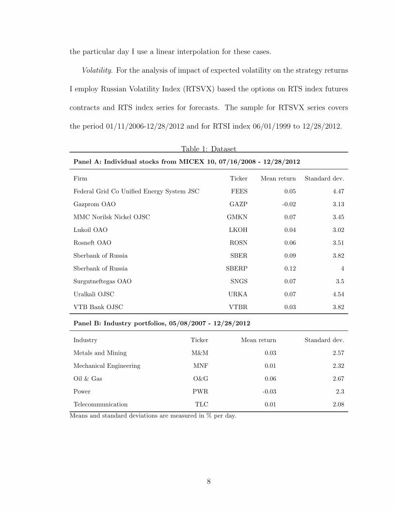
Individual stocks. First, the dataset includes a hourly data for a fixed list of
individual stocks currently3 included in the MICEX10 index, which highlights the
changes in most liquid instruments in the equity market. The sample covers the
period from 07/16/2008 to 12/28/2012. The period starts at the latest date when
currently included stocks began trading. Panel A in Table 1 shows these stocks
involved in the analysis. Second, for the further analysis I employ daily data for a
list of stocks which changes according to MICEX 10 index updates4. I know in what
stocks I will have a position tomorrow. I assume if the index rebalances tomorrow
and some stocks will get out or other liquid stock will not be traded tomorrow I do
not include these stocks in the portfolio formation. The sample for this part of the
dataset is from 06/01/1999 to 12/28/2012, includes 26 stocks (even currently not
traded).
Industry portfolios. Following Nagel (2012) and Lewellen (2002) I use daily data
for industry portfolios, but proxied by MICEX industry indices. Five core MICEX
indices being tracked since 05/08/2007 are analyzed (Panel B in Table 1). The sample
covers the period from this date to 12/28/2012.
Risk-free rate. I employ Moscow InterBank Offered Rate overnight return 5 daily
data over the period from 08/01/2000 to 12/28/2012. If the rate is not available for
3Updated on 09/01/2013.4http://rts.micex.ru/a17225http://www.cbr.ru/mkr base/
7
Page 8
the particular day I use a linear interpolation for these cases.
Volatility. For the analysis of impact of expected volatility on the strategy returns
I employ Russian Volatility Index (RTSVX) based the options on RTS index futures
contracts and RTS index series for forecasts. The sample for RTSVX series covers
the period 01/11/2006-12/28/2012 and for RTSI index 06/01/1999 to 12/28/2012.
Table 1: Dataset
Panel A: Individual stocks from MICEX 10, 07/16/2008 - 12/28/2012
Firm Ticker Mean return Standard dev.
Federal Grid Co Unified Energy System JSC FEES 0.05 4.47
Gazprom OAO GAZP -0.02 3.13
MMC Norilsk Nickel OJSC GMKN 0.07 3.45
Lukoil OAO LKOH 0.04 3.02
Rosneft OAO ROSN 0.06 3.51
Sberbank of Russia SBER 0.09 3.82
Sberbank of Russia SBERP 0.12 4
Surgutneftegas OAO SNGS 0.07 3.5
Uralkali OJSC URKA 0.07 4.54
VTB Bank OJSC VTBR 0.03 3.82
Panel B: Industry portfolios, 05/08/2007 - 12/28/2012
Industry Ticker Mean return Standard dev.
Metals and Mining M&M 0.03 2.57
Mechanical Engineering MNF 0.01 2.32
Oil & Gas O&G 0.06 2.67
Power PWR -0.03 2.3
Telecommunication TLC 0.01 2.08
Means and standard deviations are measured in % per day.
8
Page 9
2.2 Methodology
Portfolio construction. I consider the trading strategy examined by Lehmann (1990).
At the end of the period t-1 the weight for stock i for holding the position at the
period t in the portfolio is given by
wit =rit−1 − rmt−1∑N
i=1 | rit−1 − rmt−1 |, (1)
where rmt = 1N
∑Ni=1 r
it is the equal-weighted market index return, which refers to the
market component. Similar to Nagel (2012) assuming 100% margin requirements,
the denominator in Equation (1) scales the capital invested per trade to 1 ruble with
50% long and short positions. Hence, total return at the period t for the portfolio is
given by
Rt =
∑Ni=1 r
it(r
it−1 − rmt−1)∑N
i=1 | rit−1 − rmt−1 |.
This strategy has an advantage of clear interpretation as equally short and long as
well as the strategy requires 1 ruble of capital per trade. This is crucial point when
strategy results with exchange fees are compared.
Effect decomposition. My focus is on the strategy with one day for both lookback
and holding periods. For the sources of the cross-sectional momentum the framework
of Lo and MacKinlay (1988) is applied. Instead of using weights scaled by the random
term in Equation (1) of Lehmann (1990) I follow Lewellen (2002) and Moskowitz, Ooi,
and Pedersen (2012) who apply Lo and MacKinlay (1988) approach for the portfolio
construction and expected portfolio profit decomposition. The portfolio weights for
the day t and the stock i are:
wit =1
N(rit−1 − rmt−1).
9
Page 10
Total portfolio return is given by
Rt =1
N
N∑i=1
rit(rit−1 − rmt−1).
Assuming unconditional means of the assets 1,2,...,N are equal to µ = (µ1, ..., µN)′
and the first order autocovariance matrix is Ω, the expected portfolio return is fol-
lowing:
E(Rt) = E
1
N
N∑i=1
ritrit−1 −
1
N
N∑i=1
rit
[1
N
N∑j=1
rjt−1
] =1
Ntr(Ω)− 1
N21′Ω1 + σ2
µ =
=N − 1
N2tr(Ω)− 1
N2[1′Ω1− tr(Ω)] + σ2
µ, (2)
where σ2µ = 1
N
∑Ni=1(µi − 1
N
∑Np=1 µp)
2 is a cross-sectional variance of the expected
mean returns. Terms in Equation (2) are rearranged to separate the sources of the
expected portfolio return due to the diagonals and off-diagonals of the autocovariance
matrix Ω.
Thus, there are three drivers of the strategy returns: own autocovariances of
stocks (diagonals, tr(Ω)), cross autocovariances (off-diagonals, 1′Ω 1 − tr(Ω)), and
cross-sectional variance of the expected mean returns.
The expected portfolio return is positive if, first, there are positive own autocovari-
ances of stocks, second, cross autocovariances are negative or less in magnitude than
own autocovariances, third, cross-sectional variance of the expected mean returns is
high. The reverse is true to get negative returns.
First, possible positive own autocovariances of stocks (diagonals, tr(Ω)) imply
that the stock with high return yesterday is more likely to generate higher returns
today. Second, in case of negative cross autocovariances (off-diagonals, 1′Ω 1− tr(Ω))
10
Page 11
yesterday’s higher gains for the particular stock lead to lower returns for other stocks
today. Third, even if Ω = 0, i.e the lack of serial and cross-sectional predictability,
and assuming µ is not zero the expected portfolio profit is positive as the investor
tends to buy winners with high unconditional means and shorting the opposite.
3 Empirical Implementation and Results
3.1 Strategy performance
For every day I have a set of assets and get simple returns from closing prices to
calculate weights, which are used in the holding period. The returns for the portfolio
are calculated close-to-close for every period.
Since the short-selling ban was adopted from 09/17/20086 to 06/15/20097, I ex-
clude short-selling trades during this period. Instead of short selling, the investor just
reserves 50% of the capital in cash. The strategy from dollar neutral becomes 50%
long.
Lookback period is defined as the number of lags used to compute weights for
portfolio construction. Holding period is defined as the number of days the investor
holds the portfolio. As emphasis is given to short-term frequencies portfolio returns
are calculated for both lookback and holding periods from one to five days (one week).
If several portfolios are active at the same time I compute average returns of them
similar to Moskowitz, Ooi, and Pedersen (2012).
6http://old.ffms.ru/document.asp?ob no=1442597http://old.ffms.ru/document.asp?ob no=194504
11
Page 12
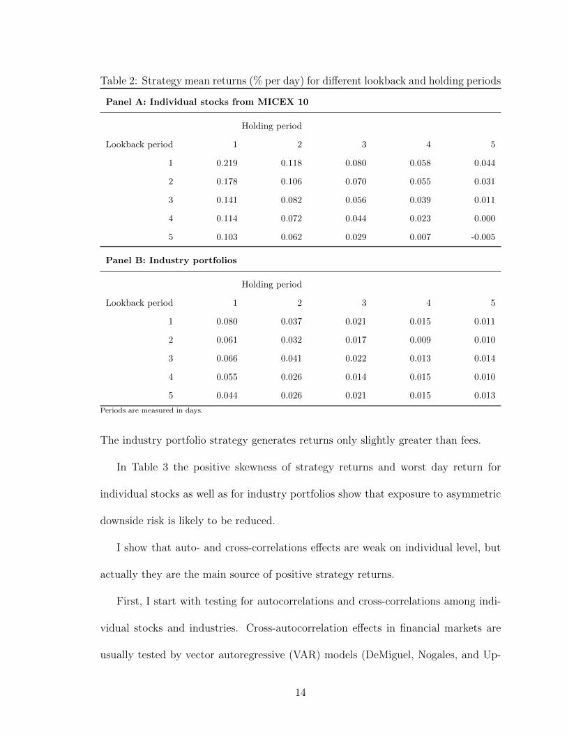
Table 2 reports results for various periods of returns for calculating weights and
days of holding the trading position. There is a clear pattern, where trading strat-
egy returns drop when lookback and holding periods increase. These findings might
suggest partial stock reversals over the long-term. Slightly profitable reversals can be
discovered for individual stocks at weekly frequencies (five days for both periods).
Surprisingly, my evidence of profitable short-term momentum on the Russian stock
market is opposite to Nagel (2012) who finds short-term reversals on the U.S. market
for the same frequency. The author also states that long-lived private information is
likely to induce negative returns from the reversal strategy in the short-term. The in-
teresting pattern of declining profits when holding periods increases supports findings
of Hong and Stein (1999). In their model this effect of high short-term momentum
profits is called an underreaction. This is a result of the gradual diffusion of pri-
vate information and failure of one market participants group (“newswatchers”) to
exploit this fact. Next, declining momentum profits refer to results of other market
participants group (“momentum traders”) which overshoots prices causing them to
overreact. Thus, one the ideas behind my evidence can be that private information
moves slowly among Russian investors.
The further analysis focuses on one day for the lookback and holding periods
as the most profitable combination. Table 3 provides more detailed results for this
combination. Figure 1 graphically shows the performance of the trading strategies.
Figure 1 shows a consistent positive strategy performance and only a huge drop in
strategy profits at the beginning of the financial crisis.
First, Panel A in Table 3 shows that mean returns from the individual liquid stocks
12
Page 13
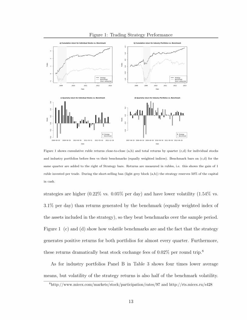
Figure 1: Trading Strategy Performance
2009 2010 2011 2012 2013
−1
01
23
Date
Rub
le
a) Cumulative return for Individual Stocks vs. Benchmark
StrategyBenchmarkShort−selling ban
2008 2009 2010 2011 2012 2013
−1.
0−
0.5
0.0
0.5
1.0
1.5
Date
Rub
le
b) Cumulative return for Industry Portfolios vs. Benchmark
StrategyBenchmarkShort−selling ban
2008−09−30 2009−06−30 2010−06−30 2011−03−31 2012−03−30 2012−12−28
c) Quarterly return for Individual Stocks vs. Benchmark
Date
Rub
le
−0.
4−
0.2
0.0
0.2
0.4
0.6
StrategyBenchmark
2007−06−29 2008−06−30 2009−06−30 2010−06−30 2011−06−30 2012−06−29
d) Quarterly return for Industry Portfolios vs. Benchmark
Date
Rub
le
−0.
4−
0.2
0.0
0.2
StrategyBenchmark
Figure 1 shows cumulative ruble returns close-to-close (a,b) and total returns by quarter (c,d) for individual stocks
and industry portfolios before fees vs their benchmarks (equally weighted indices). Benchmark bars on (c,d) for the
same quarter are added to the right of Strategy bars. Returns are measured in rubles, i.e. this shows the gain of 1
ruble invested per trade. During the short-selling ban (light grey block (a,b)) the strategy reserves 50% of the capital
in cash.
strategies are higher (0.22% vs. 0.05% per day) and have lower volatility (1.54% vs.
3.1% per day) than returns generated by the benchmark (equally weighted index of
the assets included in the strategy), so they beat benchmarks over the sample period.
Figure 1 (c) and (d) show how volatile benchmarks are and the fact that the strategy
generates positive returns for both portfolios for almost every quarter. Furthermore,
these returns dramatically beat stock exchange fees of 0.02% per round trip.8
As for industry portfolios Panel B in Table 3 shows four times lower average
means, but volatility of the strategy returns is also half of the benchmark volatility.
8http://www.micex.com/markets/stock/participation/rates/97 and http://rts.micex.ru/s428
13
Page 14
Table 2: Strategy mean returns (% per day) for different lookback and holding periods
Panel A: Individual stocks from MICEX 10
Holding period
Lookback period 1 2 3 4 5
1 0.219 0.118 0.080 0.058 0.044
2 0.178 0.106 0.070 0.055 0.031
3 0.141 0.082 0.056 0.039 0.011
4 0.114 0.072 0.044 0.023 0.000
5 0.103 0.062 0.029 0.007 -0.005
Panel B: Industry portfolios
Holding period
Lookback period 1 2 3 4 5
1 0.080 0.037 0.021 0.015 0.011
2 0.061 0.032 0.017 0.009 0.010
3 0.066 0.041 0.022 0.013 0.014
4 0.055 0.026 0.014 0.015 0.010
5 0.044 0.026 0.021 0.015 0.013
Periods are measured in days.
The industry portfolio strategy generates returns only slightly greater than fees.
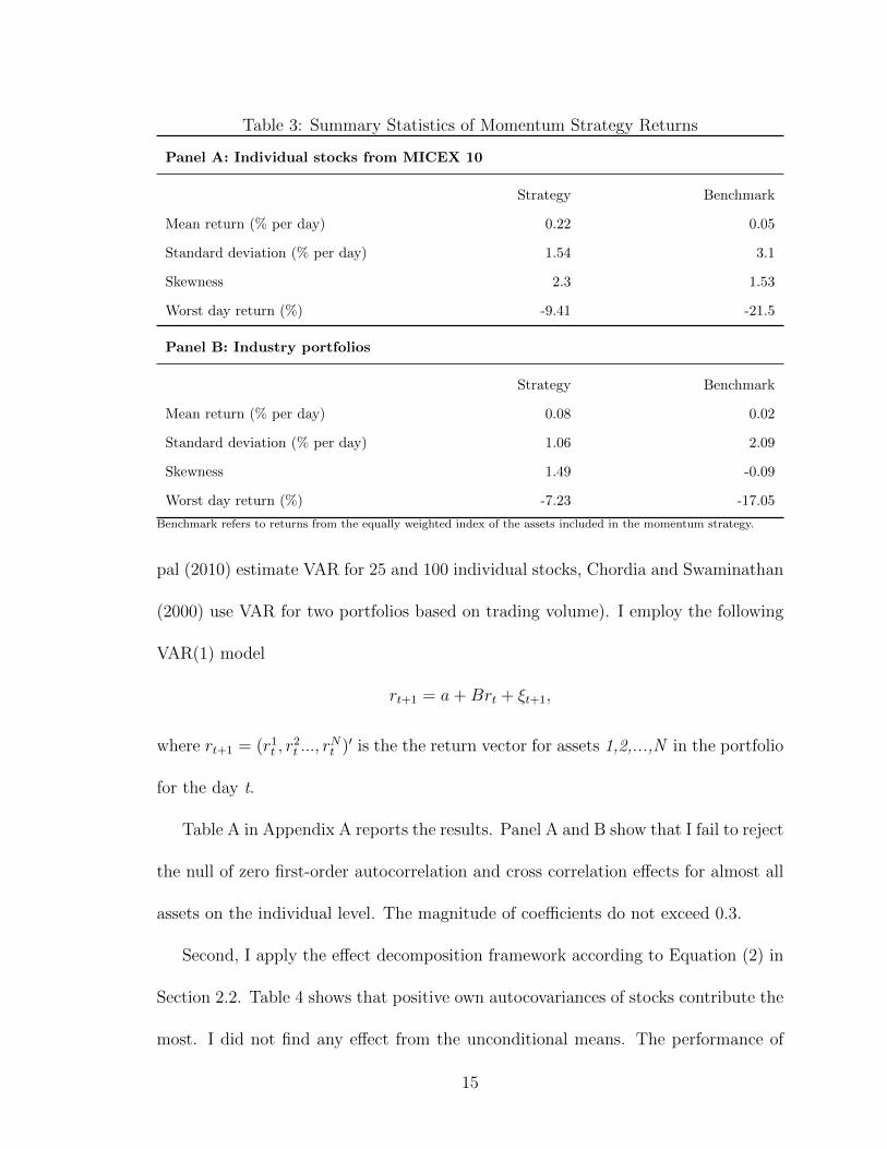
In Table 3 the positive skewness of strategy returns and worst day return for
individual stocks as well as for industry portfolios show that exposure to asymmetric
downside risk is likely to be reduced.
I show that auto- and cross-correlations effects are weak on individual level, but
actually they are the main source of positive strategy returns.
First, I start with testing for autocorrelations and cross-correlations among indi-
vidual stocks and industries. Cross-autocorrelation effects in financial markets are
usually tested by vector autoregressive (VAR) models (DeMiguel, Nogales, and Up-
14
Page 15
Table 3: Summary Statistics of Momentum Strategy Returns
Panel A: Individual stocks from MICEX 10
Strategy Benchmark
Mean return (% per day) 0.22 0.05
Standard deviation (% per day) 1.54 3.1
Skewness 2.3 1.53
Worst day return (%) -9.41 -21.5
Panel B: Industry portfolios
Strategy Benchmark
Mean return (% per day) 0.08 0.02
Standard deviation (% per day) 1.06 2.09
Skewness 1.49 -0.09
Worst day return (%) -7.23 -17.05
Benchmark refers to returns from the equally weighted index of the assets included in the momentum strategy.
pal (2010) estimate VAR for 25 and 100 individual stocks, Chordia and Swaminathan
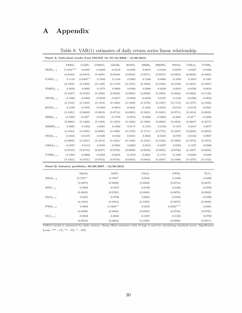
(2000) use VAR for two portfolios based on trading volume). I employ the following
VAR(1) model
rt+1 = a+Brt + ξt+1,
where rt+1 = (r1t , r
2t ..., r
Nt )′ is the the return vector for assets 1,2,...,N in the portfolio
for the day t.
Table A in Appendix A reports the results. Panel A and B show that I fail to reject
the null of zero first-order autocorrelation and cross correlation effects for almost all
assets on the individual level. The magnitude of coefficients do not exceed 0.3.
Second, I apply the effect decomposition framework according to Equation (2) in
Section 2.2. Table 4 shows that positive own autocovariances of stocks contribute the
most. I did not find any effect from the unconditional means. The performance of
15
Page 16
Table 4: Daily momentum return decomposition
Auto Cross Means Total
Individual stocks 0.0091∗∗ -0.0033 0.0000 0.0058∗∗∗
(0.0051) (0.0041) — (0.0016)
Industry portfolios 0.0047∗∗∗ -0.0036∗∗∗ 0.0000 0.0011∗∗∗
(0.0017) (0.0015) — (0.0004)
Standard errors are in parentheses. Mean returns and standard errors are measured in percent, however the position
size changes over time. Auto referes to the own autocovariance component, Cross is the profit component attributed to
cross-serial covariance, and Means refers to the unconditional expected returns component. Newey-West long variance
is used for calculating standard errors. Significance levels: *** - 1%, ** - 5%, * - 10%.
the momentum strategy also degrades due to the lack of relative winners-losers effect,
because cross autocovariances are slightly positive. This performance deterioration
is more prominent and statistically significant among industry portfolios. To test for
significance I follow Pan, Liano, and Huang (2004) and construct z-statistics which
are standard normal under the null hypothesis of no correspondent effect.
Thus, positive autocorrelation is the driver of positive momentum strategy re-
turns, despite the fact of no significant difference of individual stocks autocorrelation
from zero. Lewellen (2002) claims that the underreaction is likely to induce positive
autocorrelation and cross-serial correlation among portfolios. The provided evidence
of profitable short-term mementum on Russian stock market and partial reversal over
the larger holding period might be consistent with an underreaction theory and other
behavioral theories implying these patterns in returns.
Now I employ the longer version of the individual stocks dataset with varying
stocks in my portfolio and extended sample period.
16
Page 17
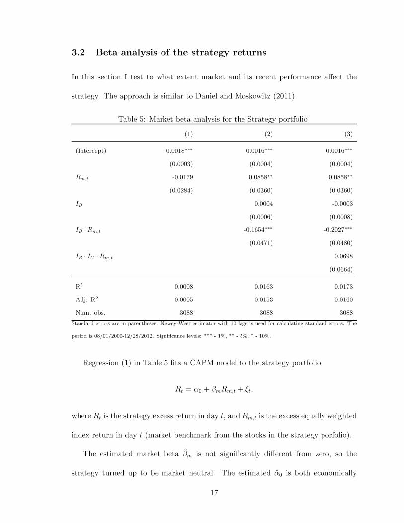
3.2 Beta analysis of the strategy returns
In this section I test to what extent market and its recent performance affect the
strategy. The approach is similar to Daniel and Moskowitz (2011).
Table 5: Market beta analysis for the Strategy portfolio
(1) (2) (3)
(Intercept) 0.0018∗∗∗ 0.0016∗∗∗ 0.0016∗∗∗
(0.0003) (0.0004) (0.0004)
Rm,t -0.0179 0.0858∗∗ 0.0858∗∗
(0.0284) (0.0360) (0.0360)
IB 0.0004 -0.0003
(0.0006) (0.0008)
IB ·Rm,t -0.1654∗∗∗ -0.2027∗∗∗
(0.0471) (0.0480)
IB · IU ·Rm,t 0.0698
(0.0664)
R2 0.0008 0.0163 0.0173
Adj. R2 0.0005 0.0153 0.0160
Num. obs. 3088 3088 3088
Standard errors are in parentheses. Newey-West estimator with 10 lags is used for calculating standard errors. The
period is 08/01/2000-12/28/2012. Significance levels: *** - 1%, ** - 5%, * - 10%.
Regression (1) in Table 5 fits a CAPM model to the strategy portfolio
Rt = α0 + βmRm,t + ξt,
where Rt is the strategy excess return in day t, and Rm,t is the excess equally weighted
index return in day t (market benchmark from the stocks in the strategy porfolio).
The estimated market beta βm is not significantly different from zero, so the
strategy turned up to be market neutral. The estimated α0 is both economically
17
Page 18
large (0.18% per day) and statistically significant, therefore the strategy generates a
significant premium on top of market returns.
Regression (2) in Table 5 fits a CAPM model conditional on the recent short-term
market performance using bear-week indicator IB
Rt = (α0 + αBIB) + (βm + βBIB)Rm,t + ξt,
where additional variable is IB, an ex-ante Bear-week dummy variable. The indicator
is one if the index five days return up to the close of day t− 1 is negative, and is zero
otherwise.
This specification tries to capture differences in expected alpha and beta of the
strategy after the short-term negative market performance. First, the point estimate
αB is not statistically different from zero and the strategy alpha α0 remains positive.
Second, the results show a decrease in market beta after a bear week (βB is negative
with p-value less than 1%). This is consistent with longer term momentum strategy as
in Daniel and Moskowitz (2011) and Grundy and Martin (2001) who find a negative
change in market beta in bear markets. After a bear week startegy beta declines and
if the market rebounds the strategy does not capture this return, but in the crisis if
the market decline continues the strategy slightly benefits from the negative beta.
Regression (3) in Table 5 fits a model to capture the extent to which the up- and
down-market betas of the strategy portfolio differ
Rt = (α0 + αBIB) + (βm + IB(βB + βU,BIB))Rm,t + ξt,
where additional variable is IU , a current Up-day dummy. This indicator is not
ex-ante, i.e. it is one if the index return in day t is positive, and is zero otherwise.
18
Page 19
This specification could assess the optionality of the strategy. In other words, I
assess nonlinearity of the strategy payoff by testing for changes in beta given the sign
of the current market return. Results show no significant optionality of the strategy
payoff conditional on the recent market poor performance.
In addition, I test for the optionality of top winner and loser stocks from my basic
portfolio separately. The idea behind this is to get an idea of market exposure of long
and short parts. I construct weighted portfolios based on winners and losers parts of
the strategy according to the positive and negative weights in the original strategy
portfolio, adjusting to have 100% of capital employed in the strategy.
Table 6: Market beta analysis for Winners and Losers portfolios
Winners (only long) Losers (only short)
(Intercept) 0.0013∗∗ 0.0016∗∗∗
(0.0006) (0.0003)
IB -0.0001 -0.0005
(0.0008) (0.0010)
Rm,t 1.1581∗∗∗ -0.9867∗∗∗
(0.0635) (0.0204)
IB ·Rm,t -0.2418∗∗∗ -0.1623∗∗∗
(0.0706) (0.0510)
IB · IU ·Rm,t 0.1119∗ 0.0253
(0.0625) (0.0933)
R2 0.5807 0.7192
Adj. R2 0.5802 0.7188
Num. obs. 3088 3088
Standard errors are in parentheses. Newey-West estimator with 10 lags is used for calculating standard errors. The
period is 08/01/2000-12/28/2012. Significance levels: *** - 1%, ** - 5%, * - 10%.
Regressions in Table 6 show significant alphas and market betas. Thus, both
19
Page 20
winners and losers parts generate strategy excess return. First, market betas differ
in magnitude for winners and losers. The winners portfolio turned out to be a higher
beta portfolio conditional on the positive recent market performance. Second, the
interesting pattern here that after a bear week betas of both winners and losers
decline. The losers portfolio becomes more aggressive and the long portfolio gains a bit
of hedge in the case of continuation of the negative recent market performance. Third,
there is a borderly significant positive optionality coefficient βU,B for the winners
portfolio. This means that after a bear week the winner portfolio gains sort of long
call property. After a bear week if the decline continues the winner portfolio beta
is β0 + βB = 0.92 and if there is a reversal β0 + βB + βB,U = 1.03. Thus, after a
bear week the winners portfolio performance slighltly refers to a long gamma and a
positive delta properties like a long call option.
3.3 Volatility and momentum returns
In the Section 3.2 I show a slight optionality embedded in long only (winners) portfo-
lio and variablity of beta conditional on the recent poor market performance. In this
section I’d like to test whether a volaility as market turmoil indicator forecasts strat-
egy returns and I try to explore whether the strategy harvests volatility risk premium.
If there is an impact of turmoil anticipation on information diffusion, strategy returns
will be significantly more likely to change. First, similarly to Daniel and Moskowitz
(2011) I test to what extent estimated market volatility forecasts future momentum
returns. I also test not only the influence of the expected variance component but the
20
Page 21
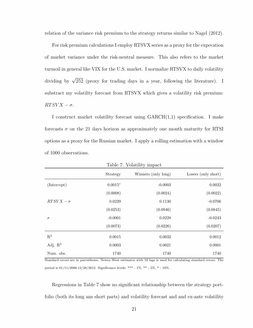
relation of the variance risk premium to the strategy returns similar to Nagel (2012).
For risk premium calculations I employ RTSVX series as a proxy for the expecation
of market variance under the risk-neutral measure. This also refers to the market
turmoil in general like VIX for the U.S. market. I normalize RTSVX to daily volatility
dividing by√
252 (proxy for trading days in a year, following the literature). I
substract my volatility forecast from RTSVX which gives a volatility risk premium:
RTSV X − σ.
I construct market volatility forecast using GARCH(1,1) specification. I make
forecasts σ on the 21 days horizon as approximately one month maturity for RTSI
options as a proxy for the Russian market. I apply a rolling estimation with a window
of 1000 observations.
Table 7: Volatility impact
Strategy Winners (only long) Losers (only short)
(Intercept) 0.0015∗ -0.0003 0.0032
(0.0008) (0.0024) (0.0022)
RTSV X − σ 0.0239 0.1130 -0.0706
(0.0253) (0.0946) (0.0845)
σ -0.0001 0.0228 -0.0243
(0.0073) (0.0226) (0.0207)
R2 0.0015 0.0032 0.0012
Adj. R2 0.0003 0.0021 0.0001
Num. obs. 1740 1740 1740
Standard errors are in parentheses. Newey-West estimator with 10 lags is used for calculating standard errors. The
period is 01/11/2006-12/28/2012. Significance levels: *** - 1%, ** - 5%, * - 10%.
Regressions in Table 7 show no significant relationship between the strategy port-
folio (both its long ans short parts) and volatility forecast and and ex-ante volatility
21
Page 22
risk premium. The results differ from Nagel (2012) who find the evidence that both
expected volatility component and volatility risk premium forecast short-term re-
versals on the U.S. stock market. Thus, the strategy does not capture volatility risk
premium and the anticipation of market turmoil does not affect the strategy, therefore
the strategy does not need to be stopped in the risk-on regime.
3.4 Robustness of results
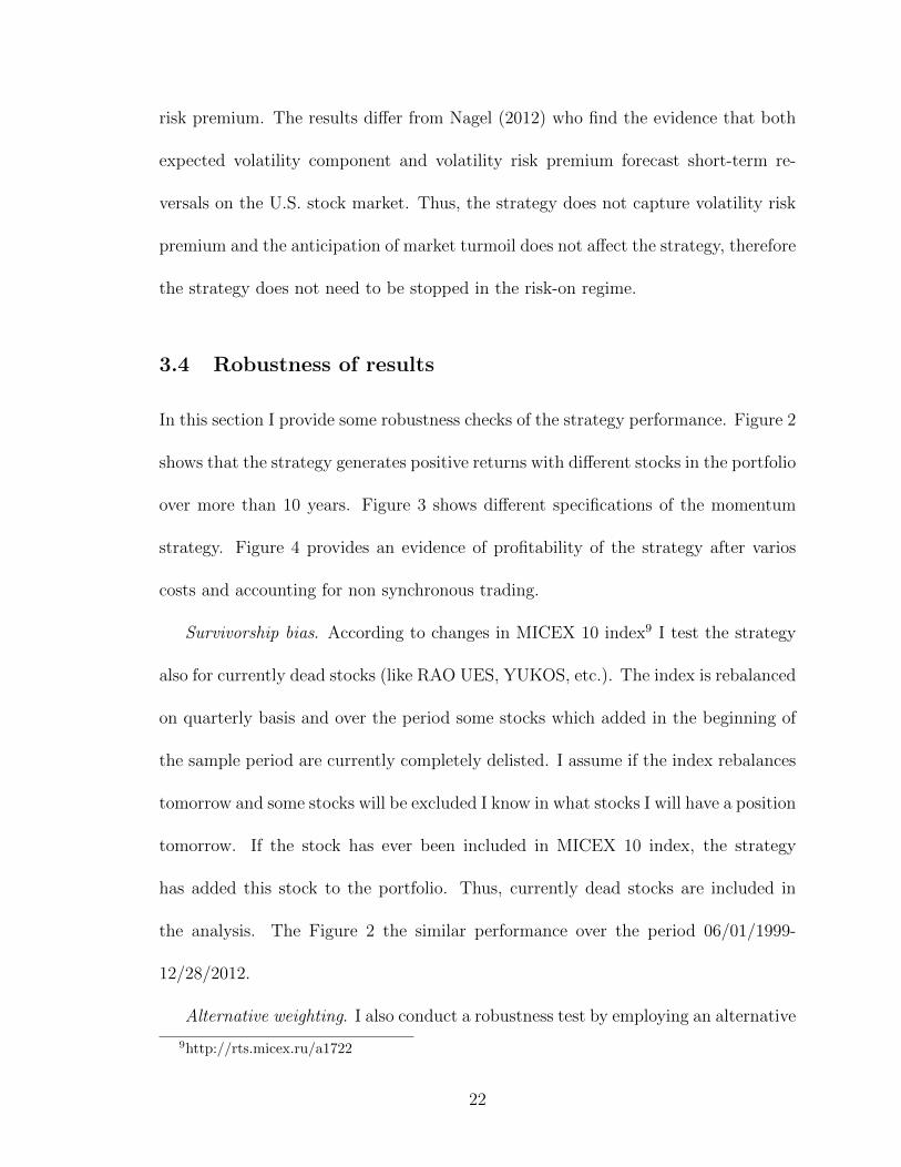
In this section I provide some robustness checks of the strategy performance. Figure 2
shows that the strategy generates positive returns with different stocks in the portfolio
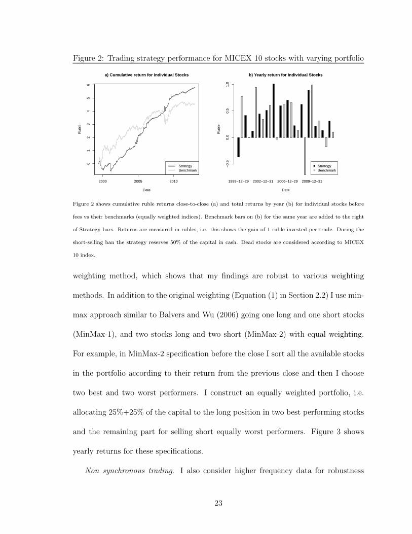
over more than 10 years. Figure 3 shows different specifications of the momentum
strategy. Figure 4 provides an evidence of profitability of the strategy after varios
costs and accounting for non synchronous trading.
Survivorship bias. According to changes in MICEX 10 index9 I test the strategy
also for currently dead stocks (like RAO UES, YUKOS, etc.). The index is rebalanced
on quarterly basis and over the period some stocks which added in the beginning of
the sample period are currently completely delisted. I assume if the index rebalances
tomorrow and some stocks will be excluded I know in what stocks I will have a position
tomorrow. If the stock has ever been included in MICEX 10 index, the strategy
has added this stock to the portfolio. Thus, currently dead stocks are included in
the analysis. The Figure 2 the similar performance over the period 06/01/1999-
12/28/2012.
Alternative weighting. I also conduct a robustness test by employing an alternative
9http://rts.micex.ru/a1722
22
Page 23
Figure 2: Trading strategy performance for MICEX 10 stocks with varying portfolio
2000 2005 2010
01
23
45
6
Date
Rub
lea) Cumulative return for Individual Stocks
StrategyBenchmark
1999−12−29 2002−12−31 2006−12−29 2009−12−31
b) Yearly return for Individual Stocks
Date
Rub
le
−0.
50.
00.
51.
0
StrategyBenchmark
Figure 2 shows cumulative ruble returns close-to-close (a) and total returns by year (b) for individual stocks before
fees vs their benchmarks (equally weighted indices). Benchmark bars on (b) for the same year are added to the right
of Strategy bars. Returns are measured in rubles, i.e. this shows the gain of 1 ruble invested per trade. During the
short-selling ban the strategy reserves 50% of the capital in cash. Dead stocks are considered according to MICEX
10 index.
weighting method, which shows that my findings are robust to various weighting
methods. In addition to the original weighting (Equation (1) in Section 2.2) I use min-
max approach similar to Balvers and Wu (2006) going one long and one short stocks
(MinMax-1), and two stocks long and two short (MinMax-2) with equal weighting.
For example, in MinMax-2 specification before the close I sort all the available stocks
in the portfolio according to their return from the previous close and then I choose
two best and two worst performers. I construct an equally weighted portfolio, i.e.
allocating 25%+25% of the capital to the long position in two best performing stocks
and the remaining part for selling short equally worst performers. Figure 3 shows
yearly returns for these specifications.
Non synchronous trading. I also consider higher frequency data for robustness
23
Page 24
Figure 3: Alternative trading strategies performance for MICEX 10 stocks
1999−12−29 2001−12−29 2003−12−30 2005−12−30 2007−12−28 2009−12−31 2011−12−30
Yearly return for Individual Stocks
Date
Rub
le
−0.
50.
00.
51.
0
LehmanMinMax−1MinMax−2
Figure 3 shows total returns by year for individual stocks before fees for three strategies. White bars refer to the
original strategy, black bars refer to portfolio formations based on going long top-1 (best) and and short bottom-1
(worst) performers, grey bars refer to the strategy equally weighting in long top-2 and short bottom-2 performers.
Returns are measured in rubles, i.e. this shows the gain of 1 ruble invested per trade. During the short-selling ban the
strategy reserves 50% of the capital in cash. Dead stocks are considered according to MICEX 10 index rebalancing
over the period 06/01/1999-12/28/2012.
check. I apply the fixed list of stocks here. The market closes at 18:45, I start
forming trading portfolio at 17:00 for latest available prices and calculate returns
based on 18:00 prices. I assume that starting forming portfolio from 17:00 to 18:00
yields expected entry price of 18:00. This delay solves the problem of non synchronous
trading and the issue of opening position at the market close. Figure 4 shows that
non synchronous trading is not the source of short term momentum profits.
Transaction costs. The profit is varying on the quarter basis. I substract ex-
change fees of 0.01% per transaction, indicative broker fees of 0.1% per transaction
and assuming 20% rate for borrowing for short selling. Figure 4 shows that the strat-
egy seems to be profitable. The above mentioned assumptions of ranking at 17:00
and rebalancing by 18:00 provide the time window for the position entry, therefore
execution algorithms could be used to minimize a price impact over the window.
24
Page 25
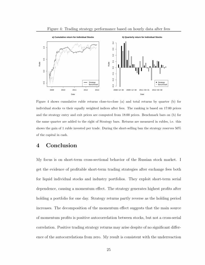
Figure 4: Trading strategy performance based on hourly data after fees
2009 2010 2011 2012 2013
−0.
50.
00.
51.
0
Date
Rub
lea) Cumulative return for Individual Stocks
StrategyBenchmark
2008−12−30 2009−12−30 2011−03−31 2012−03−30
b) Quarterly return for Individual Stocks
Date
Rub
le
−0.
3−
0.2
−0.
10.
00.
10.
20.
30.
4
StrategyBenchmark
Figure 4 shows cumulative ruble returns close-to-close (a) and total returns by quarter (b) for
individual stocks vs their equally weighted indices after fees. The ranking is based on 17:00 prices
and the strategy entry and exit prices are computed from 18:00 prices. Benchmark bars on (b) for
the same quarter are added to the right of Strategy bars. Returns are measured in rubles, i.e. this
shows the gain of 1 ruble invested per trade. During the short-selling ban the strategy reserves 50%
of the capital in cash.
4 Conclusion
My focus is on short-term cross-sectional behavior of the Russian stock market. I
get the evidence of profitable short-term trading strategies after exchange fees both
for liquid individual stocks and industry portfolios. They exploit short-term serial
dependence, causing a momentum effect. The strategy generates highest profits after
holding a portfolio for one day. Strategy returns partly reverse as the holding period
increases. The decomposition of the momentum effect suggests that the main source
of momentum profits is positive autocorrelation between stocks, but not a cross-serial
correlation. Positive trading strategy returns may arise despite of no significant differ-
ence of the autocorrelations from zero. My result is consistent with the underreaction
25
Page 26
theory, specifically, a result of the slow diffusion of news among Russian investors.
Actually, the strategy is a market neutral strategy. But I find the winners portfolio
to be a higher beta portfolio conditional a positive weekly market return but after
a week of poor market performance betas of both winners and losers decline. There
is a slight evidence of long call property embedded in the winners portfolio. I find
that expected variance component and the variance risk premium are not sources
of short-term momentum profits. Strategy performance is robust to other weighting
methods and non synchronous trading.
26
Page 27
5 References
Anatolyev, S. (2005): “A ten-year retrospection of the behavior of Russian stock
returns.,” Working paper.
Balvers, R. J., and Y. Wu (2006): “Momentum and mean reversion across na-
tional equity markets,” Journal of Empirical Finance, 13(1), 24–48.
Blitz, D., J. Huij, and M. Marten (2011): “Residual momentum,” Journal of
Empirical Finance, 18(3), 506–521.
Chordia, T., and B. Swaminathan (2000): “Trading Volume and Cross-
Autocorrelations in Stock Returns,” Journal of Finance, 55(2), 913–935.
Daniel, K., and T. Moskowitz (2011): “Momentum crashes,” Columbia Business
School Research Paper, (11-03).
de Groot, W., J. Pang, and L. Swinkels (2012): “The cross-section of stock
returns in frontier emerging markets,” Journal of Empirical Finance, 19(5), 796–
818.
DeMiguel, V., F. J. Nogales, and R. Uppal (2010): “Stock Return Serial
Dependence and Out-of-Sample Portfolio Performance,” Working Paper.
27
Page 28
Galperin, M. A., and T. V. Teplova (2012): “Dividend Investing Strategies in
the Russian Stock Market: Dogs of the Dow and Portfolios Filtered by Fundamental
Factors,” HSE Economic Journal, 16(2), 205–242.
Griffin, J. M., P. J. Kelly, and F. Nardari (2010): “Do Market Efficiency
Measures Yield Correct Inferences? A Comparison of Developed and Emerging
Markets,” Review of Financial Studies, 23(8), 3225–3277.
Grundy, B. D., and J. S. Martin (2001): “Understanding the Nature of the Risks
and the Source of Rewards to Momentum Investing,” Review of Financial Studies,
(14), 29–78.
Hong, H., and J. C. Stein (1999): “A Unified Theory of Underreaction, Mo-
mentum Trading, and Overreaction in Asset Markets,” Journal of Finance, 54(6),
2143–2184.
Jegadeesh, N., and S. Titman (1993): “Returns to Buying Winners and Selling
Losers: Implications for Stock Market Efficiency,” Journal of Finance, 48(1), 65–
91.
Lehmann, B. N. (1990): “Fads, Martingales, and Market Efficiency,” The Quarterly
Journal of Economics, 105(1), 1–28.
Lewellen, J. (2002): “Momentum and Autocorrelation in Stock Returns,” Review
of Financial Studies, 15(2), 533–564.
28
Page 29
Lo, W. A., and A. C. MacKinlay (1988): “Stock Market Prices do not Follow
Random Walks: Evidence from a Simple Specification Test,” Review of Financial
Studies, 1(1), 41–66.
Moskowitz, T., Y. H. Ooi, and L. H. Pedersen (2012): “Time series momen-
tum,” Journal of Financial Economics, 104(2), 228–250.
Nagel, S. (2012): “Evaporating Liquidity,” Review of Financial Studies, 25(7),
2005–2039.
Pan, M.-S., K. Liano, and G.-C. Huang (2004): “Industry momentum strategies
and autocorrelations in stock returns,” Journal of Empirical Finance, 11(2), 185–
202.
29
Page 30
A Appendix
Table 8: VAR(1) estimates of daily return series linear relationship
Panel A: Individual stocks from MICEX 10, 07/16/2008 - 12/28/2012
FEESt GAZPt GMKNt LKOHt ROSNt SBERt SBERPt SNGSt URKAt VTBRt
FEESt−1 0.1553∗∗∗ -0.0247 -0.0249 -0.0152 -0.0385 0.0013 -0.0149 -0.0379 0.0447 -0.0484
(0.0544) (0.0418) (0.0485) (0.0348) (0.0525) (0.0571) (0.0537) (0.0504) (0.0848) (0.0493)
GAZPt−1 0.1153 0.2459∗∗ 0.1056 0.1144 0.2362 0.1248 0.0996 0.1059 0.2455 0.1391
(0.1595) (0.1230) (0.1449) (0.1179) (0.1755) (0.1964) (0.1932) (0.1549) (0.1631) (0.1691)
GMKNt−1 0.0356 0.0693 0.1475 0.0899 0.0300 0.0368 0.0228 0.0010 -0.0536 0.0016
(0.1027) (0.0740) (0.1000) (0.0642) (0.0942) (0.0838) (0.1003) (0.0682) (0.0962) (0.1130)
LKOHt−1 -0.1083 -0.0389 -0.0639 -0.0217 -0.0639 -0.0546 0.0107 0.1524 -0.0392 -0.0634
(0.1316) (0.1233) (0.1318) (0.1250) (0.1499) (0.1570) (0.1387) (0.1113) (0.1377) (0.1292)
ROSNt−1 0.1349 -0.0705 -0.0469 -0.0674 -0.0021 -0.1645 -0.0701 -0.0118 -0.0153 -0.0501
(0.1281) (0.0662) (0.0813) (0.0714) (0.0825) (0.1061) (0.1081) (0.0711) (0.1014) (0.0935)
SBERt−1 -0.1952 -0.235∗ -0.0161 -0.1706 -0.2554 -0.0506 -0.0963 -0.2481 -0.44∗∗ -0.3282
(0.2083) (0.1248) (0.1358) (0.1270) (0.1922) (0.1862) (0.2086) (0.1634) (0.2247) (0.2571)
SBERPt−1 0.3087 0.1652 0.0361 0.1092 0.2117 0.1274 0.2748 0.1472 0.2317 0.2677
(0.1944) (0.1065) (0.0895) (0.1088) (0.1750) (0.1711) (0.1775) (0.1647) (0.2236) (0.2653)
SNGSt−1 -0.0345 -0.0175 0.0430 0.0162 -0.0011 0.0033 -0.0105 0.0705 -0.0146 0.0957
(0.0850) (0.1051) (0.1613) (0.1041) (0.1166) (0.1541) (0.1520) (0.1002) (0.1074) (0.1273)
URKAt−1 -0.0347 0.0112 0.0350 -0.0084 0.0283 0.0410 -0.0237 0.0383 0.1337 0.0308
(0.0743) (0.0710) (0.0557) (0.0730) (0.0688) (0.0642) (0.0625) (0.0746) (0.1267) (0.0625)
VTBRt−1 -0.1994 -0.0892 -0.0225 -0.0845 -0.1010 -0.0621 -0.1574 -0.1683 -0.0246 0.0398
(0.1451) (0.0741) (0.0732) (0.0716) (0.0943) (0.0944) (0.1097) (0.1088) (0.1476) (0.1152)
Panel B: Industry portfolios, 05/08/2007 - 12/28/2012
M&Mt MNFt O&Gt PWRt TLCt
M&Mt−1 0.1752∗∗ 0.1053∗ 0.0545 0.1008 0.0486
(0.0879) (0.0629) (0.0902) (0.0754) (0.0637)
MNFt−1 -0.0993 -0.0373 -0.0798 -0.0440 -0.0790
(0.0605) (0.0765) (0.0846) (0.0676) (0.0562)
O&Gt−1 0.0251 -0.0708 0.0604 -0.0532 -0.0308
(0.1052) (0.0912) (0.1399) (0.0875) (0.0839)
PWRt−1 0.0895 0.1858∗∗ 0.0276 0.2556∗∗∗ 0.0901
(0.0996) (0.0829) (0.0932) (0.0740) (0.0785)
TLCt−1 -0.0932 -0.0032 -0.1067 -0.1453 0.0792
(0.0910) (0.0694) (0.1028) (0.0909) (0.0611)
VAR(1) model is estimated for daily returns. Newey-West estimator with 10 lags is used for calculating standard errors. Significance
levels: *** - 1%, ** - 5%, * - 10%.
30