Outline Loops EFT Renormalization End Wilsonian renormalization Sourendu Gupta Mini School 2016, IACS Kolkata, India Effective Field Theories 29 February–4 March, 2016 Sourendu Gupta Effective Field Theories 2014: Lecture 2
Transcript
Outline Loops EFT Renormalization End
Wilsonian renormalization
Sourendu Gupta
Mini School 2016, IACS Kolkata, India
Effective Field Theories29 February–4 March, 2016
Sourendu Gupta Effective Field Theories 2014: Lecture 2
Outline Loops EFT Renormalization End
Outline
Outline
Spurious divergences in Quantum Field Theory
Wilsonian Effective Field Theories
Wilsonian renormalizationThe renormalization groupThe Wilsonian point of viewRG for an Euclidean field theory in D = 0Defining QFT without perturbation theory
End matter
Sourendu Gupta Effective Field Theories 2014: Lecture 2
Outline Loops EFT Renormalization End
Outline
Outline
Spurious divergences in Quantum Field Theory
Wilsonian Effective Field Theories
Wilsonian renormalizationThe renormalization groupThe Wilsonian point of viewRG for an Euclidean field theory in D = 0Defining QFT without perturbation theory
End matter
Sourendu Gupta Effective Field Theories 2014: Lecture 2
Outline Loops EFT Renormalization End
The old renormalization
We start with a Lagrangian, for example, the 4-Fermi theory:
L =1
2ψ/∂ψ − 1
2mψψ + λ(ψψ)2 + · · ·
Here all the parameters are finite. But anticipating the divergenceof perturbative expansions, we add counter-terms
Lc =1
2Aψ/∂ψ − 1
2Bmψψ + λC (ψψ)2 + · · ·
where A, B , C , etc., are chosen to cancel all divergences inamplitudes. This gives the renormalized Lagrangian
Lr =1
2ψr/∂ψr −
1
2mrψrψr + λr (ψrψr )
2 + · · ·
Clearly, ψr = Zψψ where ψr = ψ√1 + A, mr = m(1 + B)/(1 + A),
λr = λ(1 + C )/(1 + A)2, etc.. The 4-Fermi theory was called anunrenormalizable theory since an infinite number of counter-termsare needed to cancel all the divergences arising from L.
Sourendu Gupta Effective Field Theories 2014: Lecture 2
Outline Loops EFT Renormalization End
Perturbation theory: expansion of amplitudes in loops
Any amplitude in a QFT can be expanded in the number of loops.
Sourendu Gupta Effective Field Theories 2014: Lecture 2
Outline Loops EFT Renormalization End
Perturbation theory: expansion of amplitudes in loops
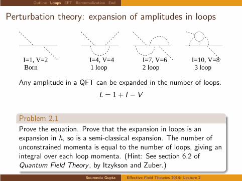
Born 1 loop 3 loopI=1, V=2 I=4, V=4
2 loop I=7, V=6 I=10, V=8
Any amplitude in a QFT can be expanded in the number of loops.
L = 1 + I − V
Sourendu Gupta Effective Field Theories 2014: Lecture 2
Outline Loops EFT Renormalization End
Perturbation theory: expansion of amplitudes in loops
Born 1 loop 3 loopI=1, V=2 I=4, V=4
2 loop I=7, V=6 I=10, V=8
Any amplitude in a QFT can be expanded in the number of loops.
L = 1 + I − V
Problem 2.1
Prove the equation. Prove that the expansion in loops is anexpansion in ~, so is a semi-classical expansion. The number ofunconstrained momenta is equal to the number of loops, giving anintegral over each loop momenta. (Hint: See section 6.2 ofQuantum Field Theory , by Itzykson and Zuber.)
Sourendu Gupta Effective Field Theories 2014: Lecture 2
Outline Loops EFT Renormalization End
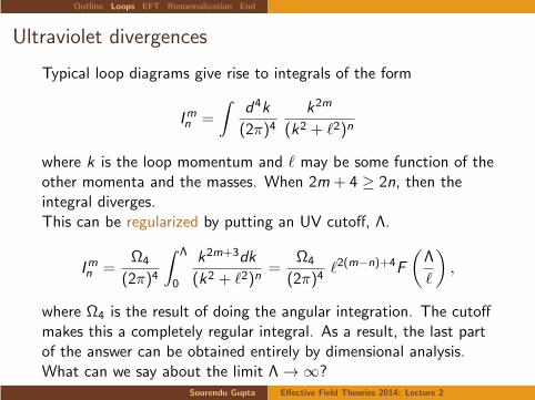
Ultraviolet divergences
Typical loop diagrams give rise to integrals of the form
Imn =
∫
d4k
(2π)4k2m
(k2 + ℓ2)n
where k is the loop momentum and ℓ may be some function of theother momenta and the masses. When 2m + 4 ≥ 2n, then theintegral diverges.This can be regularized by putting an UV cutoff, Λ.
Imn =Ω4
(2π)4
∫ Λ
0
k2m+3dk
(k2 + ℓ2)n=
Ω4
(2π)4ℓ2(m−n)+4F
(
Λ
ℓ
)
,
where Ω4 is the result of doing the angular integration. The cutoffmakes this a completely regular integral. As a result, the last partof the answer can be obtained entirely by dimensional analysis.What can we say about the limit Λ → ∞?
Sourendu Gupta Effective Field Theories 2014: Lecture 2
Outline Loops EFT Renormalization End
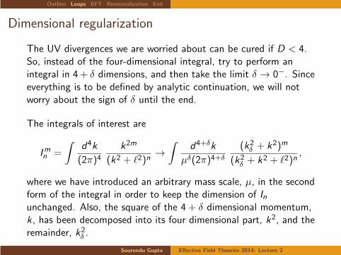
Dimensional regularization
The UV divergences we are worried about can be cured if D < 4.So, instead of the four-dimensional integral, try to perform anintegral in 4 + δ dimensions, and then take the limit δ → 0−. Sinceeverything is to be defined by analytic continuation, we will notworry about the sign of δ until the end.
The integrals of interest are
Imn =
∫
d4k
(2π)4k2m
(k2 + ℓ2)n→∫
d4+δk
µδ(2π)4+δ(k2δ + k2)m
(k2δ + k2 + ℓ2)n,
where we have introduced an arbitrary mass scale, µ, in the secondform of the integral in order to keep the dimension of Inunchanged. Also, the square of the 4 + δ dimensional momentum,k , has been decomposed into its four dimensional part, k2, and theremainder, k2δ .
Sourendu Gupta Effective Field Theories 2014: Lecture 2
Outline Loops EFT Renormalization End
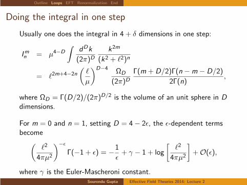
Doing the integral in one step
Usually one does the integral in 4 + δ dimensions in one step:
Imn = µ4−D
∫
dDk
(2π)Dk2m
(k2 + ℓ2)n
= ℓ2m+4−2n
(
ℓ
µ
)D−4 ΩD
(2π)DΓ(m + D/2)Γ(n −m − D/2)
2Γ(n),
where ΩD = Γ(D/2)/(2π)D/2 is the volume of an unit sphere in D
dimensions.
For m = 0 and n = 1, setting D = 4− 2ǫ, the ǫ-dependent termsbecome(
ℓ2
4πµ2
)
−ǫ
Γ(−1 + ǫ) = −1
ǫ+ γ − 1 + log
[
ℓ2
4πµ2
]
+O(ǫ),
where γ is the Euler-Mascheroni constant.Sourendu Gupta Effective Field Theories 2014: Lecture 2
Outline Loops EFT Renormalization End
Doing the integral in two steps
One can do this integral in two steps, as indicated by thedecomposition given below
I 0n =
∫
d4k
(2π)41
(2πµ)δ
∫
dδk
(k2δ + k2 + ℓ2)n,
Simply by power counting, one knows that the internal integralshould be a k-independent multiple of (k2 + ℓ2)−n+δ/2. In fact,this is most easily taken care of by the transformation of variablesk2δ = (k2 + ℓ2)x2. This gives
∫
dδk/(2πµ)δ
(k2δ + k2 + ℓ2)n=
1
(k2 + ℓ2)n
(
k2 + ℓ2
2πµ
)δ
Ωδ
∫
xδ−1dx
(1 + x2)n
where Ωδ is the angular integral in δ dimensions. The last twofactors do not depend on k , the first factor reproduces In, so theregularization must be due to the second factor.
Sourendu Gupta Effective Field Theories 2014: Lecture 2
Outline Loops EFT Renormalization End
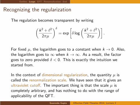
Recognizing the regularization
The regulation becomes transparent by writing
(
k2 + ℓ2
2πµ
)δ
= exp
[
δ log
(
k2 + ℓ2
2πµ
)]
.
For fixed µ, the logarithm goes to a constant when k → 0. Also,the logarithm goes to ∞ when k → ∞. As a result, the factorgoes to zero provided δ < 0. This is exactly the intuition westarted from.
In the context of dimensional regularization, the quantity µ iscalled the renormalization scale. We have seen that it gives anultraviolet cutoff. The important thing is that the scale µ iscompletely arbitrary, and has nothing to do with the range ofapplicability of the QFT.
Sourendu Gupta Effective Field Theories 2014: Lecture 2
Outline Loops EFT Renormalization End
Review problems: understanding the old renormalization
Problem 2.2: Self-study
Study the proof of renormalizability of QED to see how one identifies all
the divergences which appear at fixed-loop orders, and how it is shown
that taking care of a fixed number of divergences (through
counter-terms) is sufficient to render the perturbation theory finite. The
curing of the divergence requires fitting a small set of parameters in the
theory to experimental data (a choice of which data is to be fitted is
called a renormalization scheme). As a result, the content of a QFT is to
use some experimental data to predict others.
Problem 2.3
Follow the above steps in a 4-Fermi theory and find a 4-loop diagram
which cannot be regularized using the counter-terms shown in Lc . Would
your arguments also go through for a scalar φ4 theory? Unrenormalizable
theories require infinite amount of input data.
Sourendu Gupta Effective Field Theories 2014: Lecture 2
Outline Loops EFT Renormalization End
Outline
Outline
Spurious divergences in Quantum Field Theory
Wilsonian Effective Field Theories
Wilsonian renormalizationThe renormalization groupThe Wilsonian point of viewRG for an Euclidean field theory in D = 0Defining QFT without perturbation theory
End matter
Sourendu Gupta Effective Field Theories 2014: Lecture 2
Outline Loops EFT Renormalization End
The old renormalization
In 1929, Heisenberg and Pauli wrote down a general formulationfor QFT and noted the problem of infinities in using perturbationtheory. After 1947 the problem was considered solved. The generaloutline of the method is the following:
Analyze perturbation theory for the loop integrals which haveultraviolet divergences.
Regulate these divergences by putting an ultraviolet cutoff insome consistent way.
Identify the independent sources of divergences, and add tothe Lagrangian counter-terms which precisely cancel thesedivergences.
QFTs are called renormalizable if there are a finite number ofcounter-terms needed to render perturbation theory useful.
Use only renormalizable Lagrangians as models for physicalphenomena.
Sourendu Gupta Effective Field Theories 2014: Lecture 2
Outline Loops EFT Renormalization End
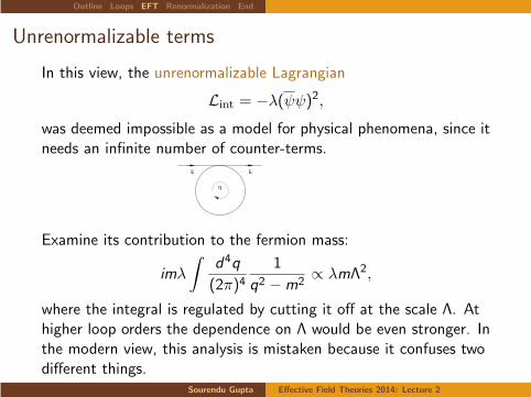
Unrenormalizable terms
In this view, the unrenormalizable Lagrangian
Lint = −λ(ψψ)2,was deemed impossible as a model for physical phenomena, since itneeds an infinite number of counter-terms.
q
k k
Examine its contribution to the fermion mass:
imλ
∫
d4q
(2π)41
q2 −m2∝ λmΛ2,
where the integral is regulated by cutting it off at the scale Λ. Athigher loop orders the dependence on Λ would be even stronger. Inthe modern view, this analysis is mistaken because it confuses twodifferent things.
Sourendu Gupta Effective Field Theories 2014: Lecture 2
Outline Loops EFT Renormalization End
Unrenormalizable terms
In this view, the unrenormalizable Lagrangian
Lint = −λ(ψψ)2,was deemed impossible as a model for physical phenomena, since itneeds an infinite number of counter-terms.
q
k k
k k
+ 1 − log(4 )γ1ε − π
Examine its contribution to the fermion mass:
imλ
∫
d4q
(2π)41
q2 −m2∝ λmΛ2,
where the integral is regulated by cutting it off at the scale Λ. Athigher loop orders the dependence on Λ would be even stronger. Inthe modern view, this analysis is mistaken because it confuses twodifferent things.
Sourendu Gupta Effective Field Theories 2014: Lecture 2
Outline Loops EFT Renormalization End
Irrelevant terms
Today the same Lagrangian is written as
Lint = − c6
Λ2(ψψ)2,
where Λ is interpreted as a scale below which one should apply thetheory.The contribution to the mass is
imc6
Λ2
∫
d4q
(2π)41
q2 −m2=
c6m3
16π2Λ2
(
−1
ǫ+ γ − 1 + log
[
m2
4πµ2
])
,
where the integral is regulated by doing it in 4− 2ǫ dimensions. Inthe MS renormalization scheme the counter-term subtracts thepole and the finite parts γ − 1− log 4π, leaving
δm
m=
c6
16π2
(m
Λ
)2log
[
m2
µ2
]
.
Sourendu Gupta Effective Field Theories 2014: Lecture 2
Outline Loops EFT Renormalization End
Separation of scales
The cutoff scale in the problem, Λ, is dissociated from therenormalization scale, µ, in dimensional regularization. This is nottrue in cutoff regularization. This separation of scales allows us torecognize two things:
There is no divergence in the limit Λ → ∞; instead thecoupling becomes irrelevant. The theory remains predictive,because the effect of these terms is bounded.
There are no large logarithms such as log(m/Λ). Theamplitudes, computed to all orders are independent of µ,although fixed loop orders are not. In practical fixedloop-order computations, it is possible to choose µ ≃ m, andreduce the dependence on this spurious scale.
Regularization schemes which do this are called mass-independentregularization. They are a crucial technical step in the newWilsonian way of thinking about renormalization.
Sourendu Gupta Effective Field Theories 2014: Lecture 2
Outline Loops EFT Renormalization End
Is cutoff regularization wrong?
All regularizations must give the same results when theperturbation theory is done to all orders. Cutoff regularization isjust more cumbersome.
Cutoff regularization retains all the problems of the old view: sincethe cutoff and renormalization scales are not separated, higherdimensional counter-terms are needed to cancel the worseningdivergences at higher loop orders. When all is computed andcancelled, the m2/Λ2 and log(m/Λ) emerge.
In mass-independent regularization schemes, higher dimensionalterms give smaller corrections because of larger powers of m/Λ.
In a renormalizable theory, since the number of counter-terms isfinite and small, the equivalence of different regularizations iseasier to see.
Sourendu Gupta Effective Field Theories 2014: Lecture 2
Outline Loops EFT Renormalization End RG flow Wilson RG Example QFT
Outline
Outline
Spurious divergences in Quantum Field Theory
Wilsonian Effective Field Theories
Wilsonian renormalizationThe renormalization groupThe Wilsonian point of viewRG for an Euclidean field theory in D = 0Defining QFT without perturbation theory
End matter
Sourendu Gupta Effective Field Theories 2014: Lecture 2
Outline Loops EFT Renormalization End RG flow Wilson RG Example QFT
The physical content of renormalization
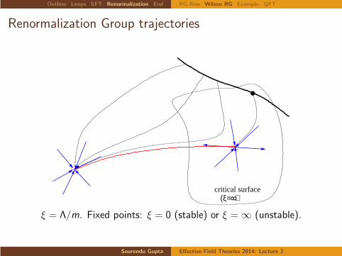
Wilson fixed his attention on the quantum field theory whichemerges as the cutoff Λ is pushed to infinity while the low-energyphysics is held fixed. According to him, one should define arenormalization group (RG) transformation as the following—
1. Integrate the momenta over [ζ, ζΛ], and perform awave-function renormalization by scaling the field to the samerange as the original fields. This changes Λ → ζΛ.
2. Find the Hamiltonian of the coarse grained field whichreproduces the dynamics of the original system. The couplingsin the Hamiltonians “flow” g(Λ) → g(ζΛ). This flow definesthe Callan-Symanzik beta-function
β(g) =∂g
∂ζ.
A fixed point of the RG has β(g) = 0.
Sourendu Gupta Effective Field Theories 2014: Lecture 2
Outline Loops EFT Renormalization End RG flow Wilson RG Example QFT
Linearized Renormalization Group transformation
Assume that there are multiple couplings Gi with beta-functionsBi . At the fixed point the values are G ∗
i . Define gi = Gi − G ∗
i .Then,
βi (G1,G2, · · · ) =∑
j
Bijgj +O(g2).
Diagonalize the matrix B whose elements are Bij . In cases ofinterest the eigenvalues, y , turn out to be real. Under an RGtransformation by a scaling factor ζ an eigenvector of B scales asv → ζyv
Eigenvectors corresponding to negative eigenvalues scale away tozero under RG, and so correspond to super-renormalizablecouplings. We have already set up the correspondence of thesewith relevant couplings. For positive eigenvalues, we findun-renormalizable couplings, i.e., irrelevant couplings. Those withzero eigenvalues are the marginal operators.
Sourendu Gupta Effective Field Theories 2014: Lecture 2
Outline Loops EFT Renormalization End RG flow Wilson RG Example QFT
Understanding the beta-function
We examine the β-function in a model field theory with a singlecoupling g . If the β-function is computed in perturbation theorythen we know its behaviour only near g = 0. But imagine that weknow it at all g .
The solution of the Callan-Symanzik equation gives us a runningcoupling, obtained by inverting the equation
ζ =
∫ g(ζ)
0
dg
β(g).
This happens since the coupling which gives a fixed physics canchange as we change the cutoff scale.
Since larger ζ means that we can examine larger momenta, thebehaviour of g(ζ) at large ζ tells us about high-energy scattering.
Sourendu Gupta Effective Field Theories 2014: Lecture 2
Outline Loops EFT Renormalization End RG flow Wilson RG Example QFT
The behaviour of model field theories
β (g)
g
a: asymptotically unfree
b: walking
d: asymptotically free
c: non−perturbative FPg*
Sourendu Gupta Effective Field Theories 2014: Lecture 2
Outline Loops EFT Renormalization End RG flow Wilson RG Example QFT
Enumerating the cases
1. Asymptotically unfree: if β(g) grows sufficiently fast, then theintegral converges. This means that the upper limit of theintegral can be pushed to infinity with ζ finite. This happenswith the one-loop expression for QED and scalar theory.
2. Walking theories: if β(g) grows slowly enough, then theintegral does not converge. As a result, g(ζ) grows veryslowly as ζ → ∞.
3. Non-perturbative fixed point: there is a new fixed point at g∗.The scaling dimensions of the fields may be very different here.
4. Asymptotic freedom: if β(g) < 0 near g = 0, then, thecoupling comes closer to g = 0 as ζ → ∞. There is no specialsignificance to β(g) changing sign at some g∗, except that itmeans that for all couplings below g∗, the renormalized theoryis asymptotically free.
Sourendu Gupta Effective Field Theories 2014: Lecture 2
Outline Loops EFT Renormalization End RG flow Wilson RG Example QFT
Wilson’s change of perspective
In a QFT we want to compute amplitudes with bounded errors,and to systematically improve the error bounds, if required. Withjust a small change in the point of view, Wilsonian renormalizationgives a new non-perturbative computing technique.
If we need amplitudes at a low momentum scale, then we can usethe RG to systematically lower the cutoff scale, by integrating overthe range [Λ/ζ,Λ]. This corresponds to coarse graining the fieldsand examining the long-distance behaviour of the theory. Now thecouplings follow the changed equation
∂g
∂ζ= −β(g).
Asymptotically unfree theories may be perturbative at longdistances; while asymptotically free theories may become highlynon-perturbative if the corresponding beta-function crosses zero atsome g∗=0.
Sourendu Gupta Effective Field Theories 2014: Lecture 2
Outline Loops EFT Renormalization End RG flow Wilson RG Example QFT
Sourendu Gupta Effective Field Theories 2014: Lecture 2
Outline Loops EFT Renormalization End RG flow Wilson RG Example QFT
Probability theory as a trivial field theory
Consider a random variate x with a probability density P(x). Inthe commonest applications x is real. One needs to compute
〈f 〉 =∫
∞
−∞
dx f (x)P(x), where 〈1〉 = 1.
Since P(x) ≥ 0, one finds S(x) = − lnP(x) is real.Define the characteristic function, Z [j ] and cumulants
Z (j) =
∫
∞
−∞
dxe−S(x)−jx , and [xn] =∂nF (j)
∂jn
∣
∣
∣
∣
j=0
,
where the generating function: F [j ] = − logZ [j ]. Note the analogyof S(x) with the action of a zero dimensional field theory, of Z (j)with the path integral and F (j) with the generating function forthe correlators. The cumulants, [xn], and are just connected partsof n-point functions of the field x . The connection between thecumulants, [xn] and the moments, 〈xn〉, is left as an exercise inMathematica.
Sourendu Gupta Effective Field Theories 2014: Lecture 2
Outline Loops EFT Renormalization End RG flow Wilson RG Example QFT
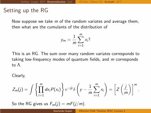
Setting up the RG
Now suppose we take m of the random variates and average them,then what are the cumulants of the distribution of
ym =1
m
m∑
i=1
xi?
This is an RG. The sum over many random variates corresponds totaking low-frequency modes of quantum fields, and m correspondsto Λ.
Clearly,
Zm(j) =
∫
m∏
i=1
dxiP(xi )
e−jyδ
(
y − 1
m
m∑
i=1
xi
)
=
[
Z
(
j
m
)]m
.
So the RG gives us Fm(j) = mF (j/m).
Sourendu Gupta Effective Field Theories 2014: Lecture 2
Outline Loops EFT Renormalization End RG flow Wilson RG Example QFT
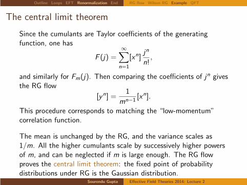
The central limit theorem
Since the cumulants are Taylor coefficients of the generatingfunction, one has
F (j) =∞∑
n=1
[xn]jn
n!,
and similarly for Fm(j). Then comparing the coefficients of jn givesthe RG flow
[yn] =1
mn−1[xn].
This procedure corresponds to matching the “low-momentum”correlation function.
The mean is unchanged by the RG, and the variance scales as1/m. All the higher cumulants scale by successively higher powersof m, and can be neglected if m is large enough. The RG flowproves the central limit theorem: the fixed point of probabilitydistributions under RG is the Gaussian distribution.
Sourendu Gupta Effective Field Theories 2014: Lecture 2
Outline Loops EFT Renormalization End RG flow Wilson RG Example QFT
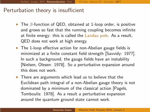
Perturbation theory is insufficient
The β-function of QED, obtained at 1-loop order, is positiveand grows so fast that the running coupling becomes infiniteat finite energy: this is called the Landau pole. As a result,QED does not work at high energy.
The 1-loop effective action for non-Abelian gauge fields isminimized at a finite constant field strength [Savvidy: 1977].In such a background, the gauge fields have an instability[Nielsen, Olesen: 1978]. So a perturbative expansion aroundthis does not work.
There are arguments which lead us to believe that theEuclidean path integral of a non-Abelian gauge theory is notdominated by a minimum of the classical action [Pagels,Tomboulis: 1978]. As a result a perturbative expansionaround the quantum ground state cannot work.
Sourendu Gupta Effective Field Theories 2014: Lecture 2
Outline Loops EFT Renormalization End RG flow Wilson RG Example QFT
What is quantum field theory?
The quantum theory of fixed number of particles can be solved inmany different ways. Perturbation theory is only one of these.
The older view of renormalization tied the definition of a quantumfield theory completely to the perturbation expansion. But sinceperturbation theory is insufficient, it became necessary to develop adefinition, i.e., a computational method, for quantum field theoryindependent of the perturbation expansion.
The Wilsonian view of renormalization yields a new way of definingcomputational techniques for quantum field theory: the method ofeffective field theory. These can be treated in perturbation theory(as in this course). Or one can treat it exactly by creating a Wilsonflow in the space of Lagrangians, as in lattice field theory.
Sourendu Gupta Effective Field Theories 2014: Lecture 2
Outline Loops EFT Renormalization End RG flow Wilson RG Example QFT
A space-time lattice
If a Green’s function has an UV divergence, then that means thatthe product of field operators separated by short distances diverges.An UV cutoff means that the shortest distances are not allowed.
A simple way to implement this is to put fields on a space-timelattice. If the lattice spacing is a, then this corresponds to an UVcutoff, Λ ≃ 1/a. Derivative operators are simple:
∂µφ(x) =1
a[φ(x + aµ)− φ(x)] .
The discretization of the derivative operator is not unique; thereare others which differ by higher powers of a. This means that thedifference between different definitions of the derivative areirrelevant operators.
Sourendu Gupta Effective Field Theories 2014: Lecture 2
Outline Loops EFT Renormalization End RG flow Wilson RG Example QFT
The reciprocal lattice: momenta
Making a lattice in space-time means putting an upper bound tothe momenta. It is also possible to make an infrared (IR) cutoff byputting the field theory in a finite box. If the box size is L = Na,and one puts periodic boundary conditions, then only the momenta2πn/(Na) are allowed. The spacing between allowed momenta is2π/(Na), the lowest momentum possible is 0, and the highestpossible momentum is 2π(N − 1)/(Na). This range is called theBrillouin zone.
Fourier transforms of fields become discrete Fourier series, andmomentum integrals become computable sums.
Problem 2.4
Explicitly construct the Fourier transforms of scalar and Diracfields with periodic and anti-periodic boundary conditions on ahypercubic lattice in 4-dimensions of size N4.
Sourendu Gupta Effective Field Theories 2014: Lecture 2
Outline Loops EFT Renormalization End RG flow Wilson RG Example QFT
Pure Higgs theory
Take the scalar field theory in Euclidean space-time:
S =
∫
d4x
[
1
2∂µφ∂
µφ− 1
2m2φ2 + λφ4
]
, (m, λ > 0),
and put it on a space-time lattice. The discretisation of thederivative in the kinetic term gives products of fields atneighbouring lattice sites. Everything else becomes an on-siteinteraction of the fields. If we take λ→ ∞, then the fields arepinned to the minimum of the potential. We can render the fieldsdimensionless using the lattice spacing a, and scale the field valueat the minimum of the potential to ±1. Then the scalar fieldtheory reduces to
S =∑
x ,µ
sxsx+µ, (sj = ±1),
which is the Ising model. (Problem 2.5: Complete thisconstruction.)
Sourendu Gupta Effective Field Theories 2014: Lecture 2
Outline Loops EFT Renormalization End
Outline
Outline
Spurious divergences in Quantum Field Theory
Wilsonian Effective Field Theories
Wilsonian renormalizationThe renormalization groupThe Wilsonian point of viewRG for an Euclidean field theory in D = 0Defining QFT without perturbation theory
End matter
Sourendu Gupta Effective Field Theories 2014: Lecture 2
David B. Kaplan, Effective Field Theories, arxiv: nucl-th/9506035;Aneesh Manohar, Effective Field Theories, arxiv: hep-ph/9606222;S. Weinberg, The Quantum Theory of Fields Vol II.
Sourendu Gupta Effective Field Theories 2014: Lecture 2
Outline Loops EFT Renormalization End
Copyright statement
Copyright for this work remains with Sourendu Gupta. However,teachers are free to use them in this form in classrooms withoutchanging the author’s name or this copyright statement. They arefree to paraphrase or extract material for legitimate classroom oracademic use with the usual academic fair use conventions.
If you are a teacher and use this material in your classes, I wouldbe very happy to hear of your experience. I will also be very happyif you write to me to point out errors.
This material may not be sold or exchanged for service, orincorporated into other media which is sold or exchanged forservice. This material may not be distributed on any other websiteexcept by my written permission.
Sourendu Gupta Effective Field Theories 2014: Lecture 2