Sparse canonical correlation analysis from apredictive point of view
Ines Wilms∗
Faculty of Economics and Business, KU Leuvenand
Christophe CrouxFaculty of Economics and Business, KU Leuven
Abstract
Canonical correlation analysis (CCA) describes the associations between two sets of vari-ables by maximizing the correlation between linear combinations of the variables in each dataset. However, in high-dimensional settings where the number of variables exceeds the samplesize or when the variables are highly correlated, traditional CCA is no longer appropriate.This paper proposes a method for sparse CCA. Sparse estimation produces linear combina-tions of only a subset of variables from each data set, thereby increasing the interpretabilityof the canonical variates. We consider the CCA problem from a predictive point of viewand recast it into a regression framework. By combining an alternating regression approachtogether with a lasso penalty, we induce sparsity in the canonical vectors. We compare theperformance with other sparse CCA techniques in different simulation settings and illustrateits usefulness on a genomic data set.
Keywords: Canonical correlation analysis; Genomic data; Lasso; Penalized regression; Sparsity.
∗Financial support from the FWO (Research Foundation Flanders) is gratefully acknowledged (FWO, contractnumber 11N9913N).
1
arX
iv:1
501.
0123
1v1
[st
at.M
E]
6 J
an 2
015
1 Introduction
The aim of canonical correlation analysis (CCA), introduced by Hotelling (1936), is to identify
and quantify linear relations between two sets of variables. CCA is used in various research fields
to study associations, for example, in physical data (Pison and Van Aelst, 2004), biomedical data
(Kustra, 2006), or environmental data (Iaci et al., 2010). One searches for the linear combinations
of each of the two sets of variables having maximal correlation. These linear combinations are called
the canonical variates and the correlations between the canonical variates are called the canonical
correlations. We refer to e.g. Johnson and Wichern (1998, Chapter 10) for more information on
canonical correlation analysis.
At the same time, we want to induce sparsity in the canonical vectors such that the linear
combinations only include a subset of the variables. Sparsity is especially helpful in analyzing
associations between high-dimensional data sets, which are commonplace today in, for example,
genetics (Qi et al., 2014) and machine learning (Sun et al., 2011; Liu et al., 2014). Therefore,
we propose a sparse version of CCA where some elements of the canonical vectors are estimated
as exactly zero, which eases interpretation. For this aim, we use the formulation of CCA as a
prediction problem.
Consider two random vectors x ∈ Rp and y ∈ Rq. We assume, without loss of generality, that
all variables are mean centered and that p ≤ q. Denote the joint covariance matrix of (x,y) by
Σ =
Σxx Σxy
Σyx Σyy
(1)
with r = rank(Σxy) ≤ p. Let A ∈ Rp×r and B ∈ Rq×r be the matrices with in their columns
the canonical vectors. The new variables u = ATx and v = BTy are the canonical variates
and the correlations between each pair of canonical variates give the canonical correlations. The
canonical vectors contained in the matrices A and B are respectively given by the eigenvectors of
the matrices
Σ−1xxΣxyΣ−1yyΣyx and Σ−1yyΣyxΣ−1xxΣxy. (2)
Both matrices have the same positive eigenvalues, the canonical correlations are given by the
positive square root of those eigenvalues.
The canonical vectors and correlations are typically estimated by taking the sample versions of
the covariances in (2) and computing the corresponding eigenvectors and eigenvalues. However, to
2
implement this procedure, we need to invert the matrices Σxx and Σyy. When the original variables
are highly correlated or when the number of variables becomes large compared to the sample size,
the estimation imprecision will be large. Moreover, when the largest number of variables in both
data sets exceeds the sample size (i.e. q ≥ n), traditional CCA cannot be performed. Vinod (1976)
proposed the canonical ridge, which is an adaptation of the ridge regression concept of Hoerl and
Kennard (1970) to the framework of CCA, to solve this problem. The canonical ridge replaces the
matrices Σ−1xx and Σ−1yy by respectively (Σxx + k1I)−1
and (Σyy + k2I)−1
. By adding the penalty
terms k1 and k2 to the diagonal elements of the sample covariance matrices, one obtains more
reliable and stable estimates when the data are nearly or exactly collinear.
Another approach is to use sparse CCA techniques. Parkhomenko et al. (2009) consider a sparse
singular value decomposition to derive sparse singular vectors. A limitation of their approach is
that sparsity in the canonical vectors is only guaranteed if Σxx and Σyy are replaced by their
corresponding diagonal matrices. A similar approach was taken by Witten et al. (2009) who
apply a penalized matrix decomposition to the cross-product matrix Σxy, but assume that one
can replace the matrices Σxx and Σyy by identity matrices. Waaijenborg et al. (2008) consider
Wold’s (1968) alternating least squares approach to CCA and obtain sparse canonical vectors using
penalized regression with elastic net. The ridge parameter of the elastic net is set to be large,
thereby, according to the authors, ignoring the dependency structure within each set of variables.
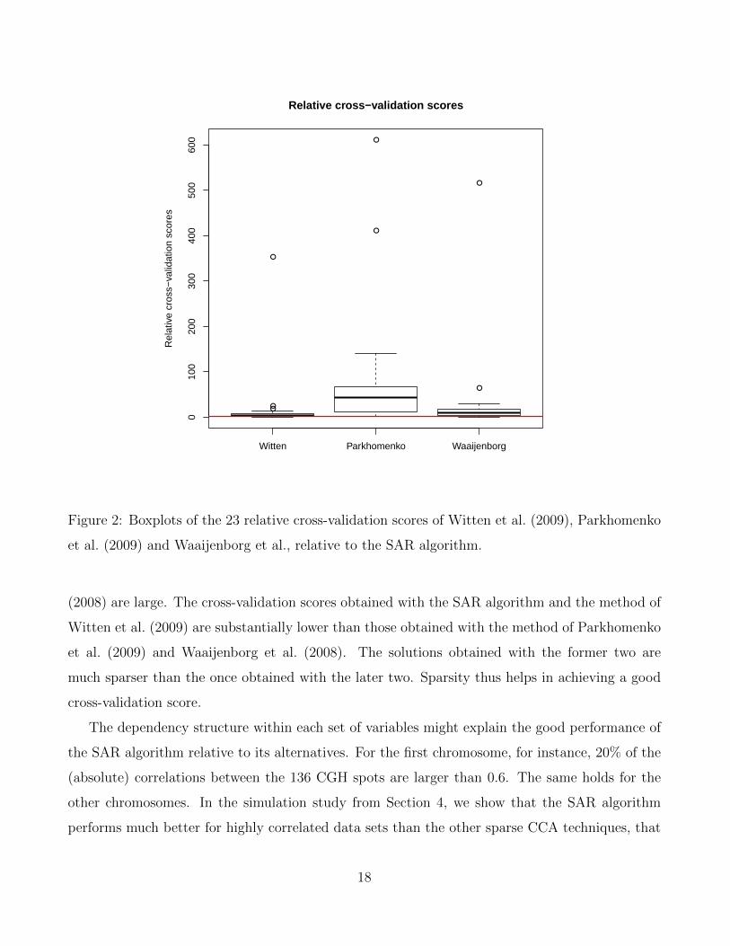
Waaijenborg et al. (2008), Witten et al. (2009), and Parkhomenko et al. (2009) all impose
covariance restrictions, i.e. ΣXX = ΣYY = I for Waaijenborg et al. (2008) and Witten et al. (2009);
diagonal matrices for Parkhomenko et al. (2009). In contrast, we propose in this paper to estimate
the canonical variates without imposing any prior covariance restrictions. Our proposed method
obtains the canonical vectors using a alternating penalized regression framework. By performing
variable selection in a penalized regression framework using the lasso penalty (Tibshirani, 1996),
we obtain sparse canonical vectors.
We demonstrate in a simulation study that our Sparse Alternating Regression (SAR) algorithm
produces good results in terms of estimation accuracy of the canonical vectors, and detection of
the sparseness structure of the canonical vectors. Especially in simulation settings when there is
a dependency structure within each set of variables, the SAR algorithm clearly outperforms the
sparse CCA methods described above. We also apply the SAR algorithm on a high-dimensional
3
genomic data set. Sparse estimation is appealing since it highlights the most important variables
for the association study.
The remainder of this article is organized as follows. In Section 2 we formulate the CCA
problem from a predictive point of view. Section 3 describes the Sparse Alternating Regression
(SAR) approach and provides details on the implementation of the algorithm. Section 4 compares
our methodology to other sparse CCA techniques by means of a simulation study. Section 5
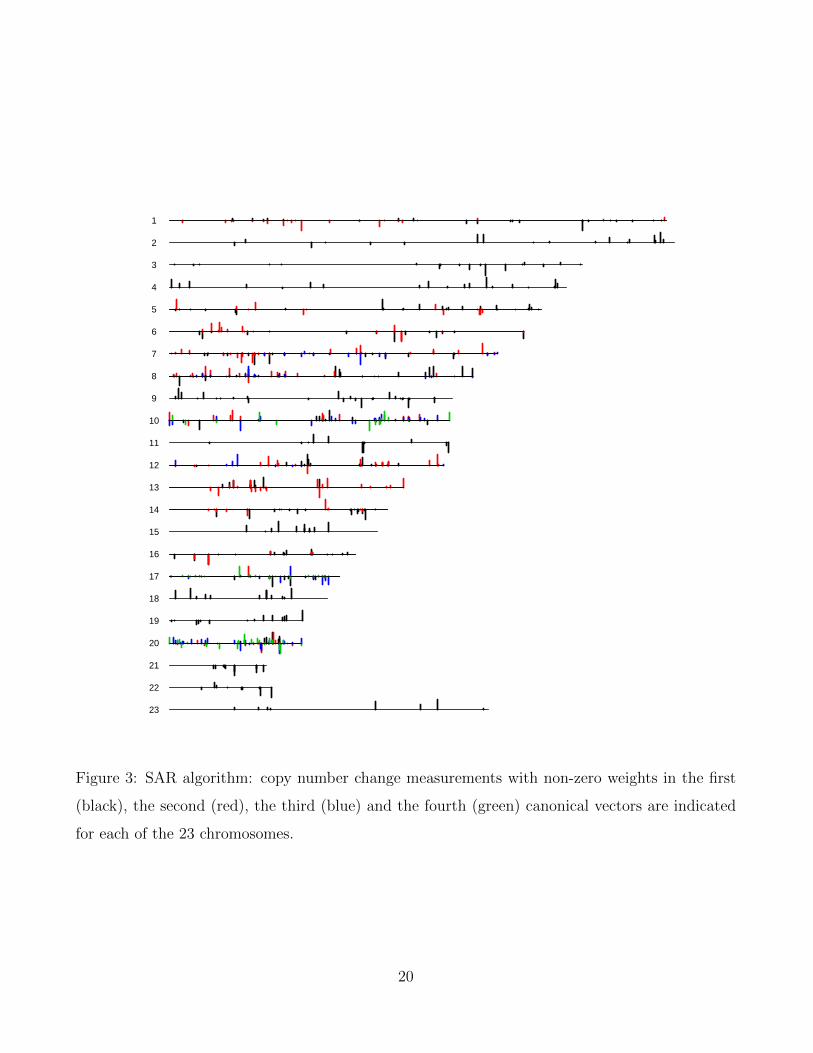
discusses the genomic data example, Section 6 concludes.
2 CCA from a predictive point of view
A characterization of the canonical vectors based on the concept of prediction is proposed by
Brillinger (1975) and Izenman (1975). Given n observations xi ∈ Rp and yi ∈ Rq (i = 1, . . . , n),
consider the optimization problem
(A, B) = argmin(A,B)∈S
n∑i=1
||ATxi −BTyi||2. (3)
We restrict the parameter space to the space S, given by
S = {(A,B) : A ∈ Rp×r,B ∈ Rq×r, rank(A) = rank(B) = r,ATΣxxA = BTΣyyB = Ir}.
We impose normalization conditions requiring the canonical variates to have unit variance and to
be uncorrelated. Brillinger (1975) proves that the objective function in (3) is minimized when A
and B contain in their columns the canonical vectors.
We build on this equivalent formulation of the CCA problem to obtain the canonical vec-
tors using an alternating regression procedure (see e.g. Wold, 1968; Branco et al., 2005). The
subsequent canonical variates are sequentially derived.
First canonical vector pair. Denote the first canonical vectors (i.e. the first columns of the
matrices A and B) by (A1,B1). Suppose we have an initial value A∗1 for the first canonical vector
in the matrix A. Then the minimization problem in (3) reduces to
B1|A∗1 = argminB1
n∑i=1
(A∗1
Txi −B1Tyi
)2, (4)
4
where we require v1 = YB1 to have unit variance. The solution to (4) can be obtained from
a multiple regression with XA∗1 as response and Y as predictor, where X = [x1, . . . ,xn]T and
Y = [y1, . . . ,yn]T .
Analogously, for a fixed value B∗1. The optimal value for A1 is obtained by a multiple regression
with YB∗1 as response and X as predictor
A1|B∗1 = argminA1
n∑i=1
(B∗1
Tyi −A1Txi
)2, (5)
where we require u1 = XA1 to have unit variance. This leads to an alternating regression scheme,
where we alternately update our estimates of the first canonical vectors until convergence. We
iterate until the angle between the estimated canonical vectors in iteration i and the respective
estimated canonical vectors in the previous iteration are both smaller than some value ε (e.g.
ε = 10−3).
Higher order canonical vector pairs. The higher order canonical variates need to be orthogonal
to the previously found canonical variates. Therefore, the alternating regression scheme is applied
on deflated data matrices (see e.g. Branco et al., 2005). For the second pair of canonical vectors,
consider the deflated matrices
X∗ = X− u1(uT1 u1)
−1uT1 X. (6)
The deflated matrix X∗ is obtained as the residuals of the multivariate regression of X on u1, the
first canonical variate. Analogously, the deflated matrix Y∗ is given by
Y∗ = Y − v1(vT1 v1)
−1vT1 Y, (7)
the residuals of the multivariate regression of Y on v1.
Using the Least Squares property, each column of X∗ is uncorrelated with the first canonical
variate u1. The second canonical variate will be a linear combination of the columns of X∗ and,
hence, will be uncorrelated to the previously found canonical variate. The same holds for Y∗. The
second canonical variate pair is then obtained by alternating between the following regressions
until convergence:
B∗2|A∗2 = argminB∗
2
n∑i=1
(A∗2
Tx∗i −B∗2Ty∗i)2
(8)
5
A∗2|B∗2 = argminA∗
2
n∑i=1
(B∗2
Ty∗i −A∗2Tx∗i)2, (9)
where we require v∗2 = Y∗B∗2 and u∗2 = X∗A∗2 to have both unit variance.
Finally, we need to express the second canonical vector pair in terms of the original data sets
X and Y. To obtain the second canonical vector A2, we regress u∗2 on X
A2 = argminA2
n∑i=1
(u∗2 −A2
Txi
)2, (10)
yielding the fitted values u2 = XA2. To obtain B2, we regress v∗2 on Y.
B2 = argminB2
n∑i=1
(v∗2 −B2
Tyi
)2. (11)
The same idea is applied to obtain the higher order canonical variate pairs.
3 Sparse alternating regressions
The canonical vectors obtained with the alternating regression scheme from Section 2 are in general
not sparse. Sparse canonical vectors are obtained by replacing the Least Squares regressions in
the alternating regression approach of Section 2 with Lasso regressions (L1-penalty). As such,
some coefficients in the canonical vectors will be set to exactly zero, thereby producing linear
combinations of only a subset of variables.
For the first pair of sparse canonical vectors, the sparse equivalents of the Least Squares
regressions in equations (4) and (5) are given by
B1|A∗1 = argminB1
n∑i=1
(A∗1
Txi −B1Tyi
)2+ λB1
q∑j=1
|bj1|,
A1|B∗1 = argminA1
n∑i=1
(B∗1
Tyi − a1Txi
)2+ λA1
p∑j=1
|aj1|,
where λB1 > 0 and λA1 > 0 are sparsity parameters, bj1 is the jth (j = 1, . . . , q) element of the
first canonical vector B1 and aj1 is the jth (j = 1, . . . , p) element of the first canonical vector A1.
The first pair of canonical variates are given by u1 = XA1 and v1 = YB1. We require both to
have unit variance.
6
To obtain the second pair of sparse canonical vectors, the same deflated matrices as in equations
(6) and (7) are used. The Least Squares regressions in equations (8) and (9) are replaced by the
Lasso regressions
B∗2|A∗2 = argminB∗
2
n∑i=1
(A∗2
Tx∗i −B∗2Ty∗i)2
+ λB∗2
q∑j=1
|b∗j2|
A∗2|B∗2 = argminA∗
2
n∑i=1
(B∗2
Ty∗i −A∗2Tx∗i)2
+ λA∗2
p∑j=1
|a∗j2|.
Finally, to express the second pair of canonical vectors in terms of the original data matrices, we
replace the Least Squares regression in (10) and (11) by the two Lasso regressions.
A2 = argminA2
n∑i=1
(u∗2 −A2
Txi
)2+ λA2
p∑j=1
|aj2|,
B2 = argminB2
n∑i=1
(v∗2 −B2
Tyi
)2+ λB2
q∑j=1
|bj2|,
yielding the fitted values u2 = XA2 and v2 = YB2. We add a lasso penalty to the above
regressions, first because the design matrix X can be high-dimensional, and second, because we
want A2 and B2 to be sparse.
A complete description of the algorithm is given below. We numerically verified that without
imposing penalization (i.e. λA,j = λB,j = 0, for j = 1, . . . , r), the traditional CCA solution
is obtained. Our numerical experiments all converged reasonably fast. Finally, note that as in
other sparse CCA proposals (Witten et al., 2009; Parkhomenko et al., 2009; Waaijenborg et al.,
2008) the sparse canonical variates are in general not uncorrelated. We do not consider this lack
of uncorrelatedness as a major flaw. The sparse canonical vectors yield an easily interpretable
basis of the space spanned by the canonical vectors. After suitable rotation of the corresponding
canonical variates, this basis can be made orthogonal (but not sparse) if one desires so.
7
Sparse Alternating Regression (SAR) Algorithm
Let X and Y be two data matrices.
1. Preliminary steps
• X0 = X− 1xT
• Y0 = Y − 1yT
2. Alternating Regressions: For l = 1, . . . , r
• If l > 1 : Deflated matrices
• Xl−1 = Xl−2 − ul−1(uTl−1ul−1)−1uT
l−1Xl−2
• Yl−1 = Yl−2 − vl−1(vTl−1vl−1)−1vT
l−1Yl−2
• Starting values
• B(0)l =
bcanridgel
||bcanridgel ||
, using the canonical vector bcanridgel obtained with the canonical ridge
• v(0)l = Yl−1B
(0)l
• From iteration s = 1 until convergence
• a(s)l = argmin
a
∑ni=1
(v(s−1)l,i − xT
l−1,ia)2
+ λa,l∑p
j=1 |aj |
• a(s)l =
a(s)l
||a(s)l ||
• u(s)l = Xl−1a
(s)l
• b(s)l = argmin
b
∑ni=1
(u(s)l,i − yT
l−1,ib)2
+ λb,l∑q
j=1 |bj |
• b(s)l =
b(s)l
||b(s)l ||
• v(s)l = Yl−1b
(s)l
• After convergence, resulting in a∗l , b∗l , u∗l and v∗l
• Ul−1 = [u1, . . . , ul−1]
• ul = u∗l − Ul−1
(UT
l−1Ul−1
)−1UT
l−1u∗l
• Al =
a∗l if l = 1
argminA
∑ni=1
(ul,i − xT
0,iA)2
+ λA,l
∑pj=1 |Aj | if l > 1
• ul = X0Al
• Vl−1 = [v1, . . . , vl−1]
• vl = v∗l − Vl−1
(VT
l−1Vl−1
)−1VT
l−1v∗l
• Bl =
b∗ if l = 1
argminB
∑ni=1
(vl,i − yT
0,iB)2
+ λB,l
∑qj=1 |Bj | if l > 1
• vl = Y0Bl
3. Final solution
• Asparse = [A1, . . . , Ar]
• Bsparse = [B1, . . . , Br]
8
Starting values. To start up the Sparse Alternating Regression (SAR) algorithm, an initial
value is required. We use the canonical vectors delivered by the canonical ridge as starting value,
which is available at no computational cost. The regularization parameters of the canonical ridge
are chosen using 5-fold cross-validation such that the average test sample canonical correlation is
maximized (Gonzalez et al., 2008).
We performed a simulation study (unreported) to assess the robustness of the SAR algorithm
to different choices of starting values. The SAR algorithm shows similar performance when either
the canonical ridge or other choices of starting values (i.e. CCA in low-dimensional settings and
randomly drawn starting values) are used.
Number of canonical variates to extract. For practical implementation, one needs to have an
idea on the number of canonical variates r to extract. Most often, only a limited number of
canonical variate pairs are truly relevant. We follow An et al. (2013) who propose the maximum
eigenvalue ratio criterion to decide on the number of canonical variates to extract. We apply the
canonical ridge and calculate the canonical correlations ρ1, . . . , ρrmax, with rmax = min(p, q). Let
kj = ρj/ρj+1 for j = 1, . . . , rmax−1. Then we set r = argmaxj kj, and extract r pairs of canonical
variates using the SAR algorithm.
Selection of sparsity parameters. In the SAR algorithm, the sparsity parameters λA,j and λB,j
(j = 1, . . . , r), which control the penalization on the respective regression coefficient matrices,
need to be selected. We select the sparsity parameters according to a minimal Bayes Information
Criterion (BIC). We solve the corresponding penalized regression problems over a range of values
and select for each the one with lowest value of
BICλA,j= −2 logLλA,j
+ kλA,jlog(n),
BICλB,j= −2 logLλB,j
+ kλB,jlog(n),
for j = 1, . . . , r. LλA,jis the estimated likelihood using sparsity parameter λA,j and kλA,j
is the
number of non-zero estimated regression coefficients. Analogously for λB,j.
9
4 Simulation Study
We compare the performance of the Sparse Alternating Regression approach with three other
sparse CCA techniques. We consider
• The Sparse Alternating Regression (SAR) algorithm detailed in Section 3.
• The sparse CCA of Witten et al. (2009)1, relying on a penalized matrix decomposition applied
to the cross-product matrix Σxy. Sparsity parameters are selected using the permutation
approach described in Gross et al. (2011).
• The sparse CCA of Parkhomenko et al. (2009)2. Sparsity parameters are selected using
5-fold cross-validation where the average test sample canonical correlation is maximized.
• The sparse CCA of Waaijenborg et al. (2008)3. The lasso parameter of the elastic net is
selected using 5-fold cross-validation such that the mean absolute difference between the
canonical correlation of the training and test sets is minimized.
We emphasize that the sparsity parameters of all methods are selected as proposed by the respec-
tive authors. The traditional CCA solution and the canonical ridge4 are computed as additional
benchmarks.
We consider several simulation schemes. For each setting we generate data matrices X and
Y according to multivariate normal distributions, with covariance matrices described in Table 1.
The number of simulations for each setting is M = 1000. In all simulation settings, the canonical
vectors have a sparse structure. In the first simulation setup (revised from Branco et al., 2005)
the covariance restrictions of Waaijenborg et al. (2008), Witten et al. (2009) and Parkhomenko
et al. (2009) (i.e. ΣXX = ΣYY = I for the former two, diagonal matrices for the latter) are
satisfied. These restrictions are violated in the second, third and fourth simulation setup. In the
third design, the number of variables is large compared to the sample size. Traditional CCA can
still be performed in this setting. In the fourth design, the number of variables in the data matrix
Y is larger than the sample size, and traditional CCA can no longer be performed.
1Available in the R package PMA (Witten et al., 2011).2Available at http://www.uhnres.utoronto.ca/labs/tritchler/.3We re-implemented the algorithm of Waaijenborg et al. (2008) in R.4Available in the R package CCA (Gonzalez and Dejean, 2009).
10
Table 1: Simulation settings
Design n p q Σxx Σyy Σxy
Uncorrelated 50 4 6 Ip Iq
3
50 0 0 0 0
01
20 0 0 0
0 0 0 0 0 0
0 0 0 0 0 0
Correlated 50 6 10 Ip
S1 0
0 I7
S2 0
0 0
with
S1ij = 0.7|i−j| S2 = 12I2
High-dimensional 50 25 40 Ip
S1 0
0 I37
S2 0
0 0
with
S1ij = 0.3|i−j| S2 = 710I2
Overparametrized 80 60 85 Ip
S1 0
0 I82
S2 0
0 0
with
S1ij = 0.3|i−j| S2 = 710I2
11
Performance measures. We compare the SAR algorithm to its alternatives and evaluate (i) the
precision accuracy of the space spanned by the estimated canonical vectors, and (ii) the detection
of the sparsity structure of the canonical vectors.
We compute for each simulation run m, with m = 1, . . . ,M , the angle θm(Am,A) between
the subspace spanned by the estimated canonical vectors contained in the columns of Am and the
subspace spanned by the true canonical vectors contained in the columns of A. Analogously for
the matrix B. The average angles are given by
θ(A,A) =1
M
M∑m=1
θm(Am,A) and θ(B,B) =1
M
M∑m=1
θm(Bm,B).
Finally, we monitor the sparsity recognition performance (e.g. Rothman et al., 2010) using the
true positive rate and the true negative rate as defined as follows
TPR(A,A) =#{(i, j) : Aij 6= 0 and Aij 6= 0}
#{(i, j) : Aij 6= 0}
TNR(A,A) =#{(i, j) : Aij = 0 and Aij = 0}
#{(i, j) : Aij = 0}.
The true positive rate indicates the number of true relevant variables detected by the estimation
procedure. The true negative rate measures the hit rate of excluding unimportant variables from
the canonical vectors. Analogue measures can be computed for the canonical vectors in the matrix
B.
Results. The simulation results on the estimation accuracy of the estimated canonical vectors
are reported in Table 2. We compute the average angle (averaged across simulation runs) between
the space spanned by the true and estimated canonical vectors. To compare the average angle
of the SAR algorithm against the other approaches, we compute p-values of a two-sided paired
t-test.
We first compare the performance of the penalized CCA techniques (i.e. canonical ridge and
sparse CCA) to the unpenalized CCA solution. The estimation accuracy of the penalized CCA
methods is significantly better compared to traditional CCA, especially in the high-dimensional
design. In the lower dimensional simulation settings (i.e. uncorrelated and correlated design),
sparse CCA techniques are still doing well since the underlying structure of the canonical vectors
is sparse.
12
Table 2: Estimation accuracy of the canonical vectors, measured by the average angle between
the subspace spanned by the true and estimated canonical vectors. P -values comparing SAR to
alternatives are all < 0.01.
Design Method θ(A,A) θ(B,B)
Uncorrelated SAR 0.008 0.019
Witten et al. (2009) 0.010 0.054
Parkhomenko et al. (2009) 0.104 0.241
Waaijenborg et al. (2008) 0.078 0.212
Canonical ridge 0.129 0.272
CCA 0.127 0.267
Correlated SAR 0.001 0.068
Witten et al. (2009) 0.061 0.299
Parkhomenko et al. (2009) 0.306 0.690
Waaijenborg et al. (2008) 0.187 0.494
Canonical ridge 0.046 0.043
CCA 0.042 0.033
High-dimensional SAR 0.212 0.305
Witten et al. (2009) 0.263 0.390
Parkhomenko et al. (2009) 0.826 0.908
Waaijenborg et al. (2008) 0.833 0.942
Canonical ridge 0.916 1.016
CCA 1.062 1.193
Overparametrized SAR 0.278 0.353
Witten et al. (2009) 0.490 0.592
Parkhomenko et al. (2009) 0.946 0.986
Waaijenborg et al. (2008) 1.137 1.181
Canonical ridge 0.916 1.211
13
Next, we compare the SAR algorithm to its sparse alternatives. In the uncorrelated design,
the covariance restrictions imposed by Waaijenborg et al. (2008), Parkhomenko et al. (2009) and
Witten et al. (2009) are satisfied. Therefore, we expect these methods to perform especially
well. Nevertheless, even in this setting, the SAR algorithm performs significantly better. In
the correlated design, the high-dimensional and the overparametrized design these covariance
restrictions are violated. Here, we see even more clearly that the SAR algorithm has a significant
advantage over its sparse alternatives. In the correlated design, for instance, the SAR algorithm
outperforms the method of Witten et al. (2009) by a factor 10 for the first canonical vector (i.e.
estimation accuracy of 0.001 against 0.061), and by a factor 5 for the second canonical vector
(i.e. estimation accuracy of 0.068 against 0.299). The gains in estimation accuracy of the SAR
algorithm compared to the other sparse CCA methods are even more outspoken.
Finally, Table 3 compares the results on sparsity recognition performance among the sparse
CCA techniques. The methods of Parkhomenko et al. (2009) and Waaijenborg et al. (2008)
produce the least sparse solution, indicated by the high true positive rates and low true negative
rates. The SAR algorithm and the method of Witten et al. (2009) tend to produce the most spare
solutions, indicated by the high true negative rates and low true positive rates. Contrary to sparse
CCA, traditional CCA and the canonical ridge don’t perform variable selection simultaneously
with model estimation. Therefore, traditional CCA and canonical ridge are not included in Table
3. All elements of the canonical vectors are estimated as non-zero, resulting in a perfect true
positive rate and zero true negative rate.
To conclude, as we can see from Table 2, in every simulation design we consider, the SAR
algorithm did perform significantly better than the other sparse CCA methods.
5 Genomic data application
In recent years, high-dimensional genomic data sets have arisen, containing thousands of gene
expression and other phenotype measurements (e.g., Chen et al., 2010; Daye et al., 2012). We
use the publicly available breast cancer data set described in Chin et al. (2006) and available in
the R package PMA (Witten et al., 2011). Comparative genomic hybridization (CGH) data (2149
variables) and gene expression data (19 672 variables) are available on 89 samples. The objective is
to identify copy number change variables that are correlated with a subset of gene expression vari-
14
Table 3: Sparsity recognition performance: true positive rate and true negative rate for canonical
vectors in the A and B matrices.
A B
Design Method TPR TNR TPR TNR
Uncorrelated SAR 0.79 0.81 0.79 0.86
Witten et al. (2009) 0.75 0.83 0.77 0.78
Parkhomenko et al. (2009) 0.94 0.22 0.93 0.25
Waaijenborg et al. (2008) 0.91 0.25 0.91 0.25
Correlated SAR 0.83 0.92 0.55 0.93
Witten et al. (2009) 0.52 0.80 0.43 0.75
Parkhomenko et al. (2009) 0.86 0.23 0.83 0.26
Waaijenborg et al. (2008) 0.86 0.31 0.83 0.31
High-dimensional SAR 0.54 0.82 0.51 0.83
Witten et al. (2009) 0.38 0.87 0.31 0.86
Parkhomenko et al. (2009) 0.72 0.35 0.70 0.40
Waaijenborg et al. (2008) 0.87 0.24 0.82 0.27
Overparametrized SAR 0.44 0.89 0.44 0.89
Witten et al. (2009) 0.37 0.82 0.32 0.82
Parkhomenko et al. (2009) 0.61 0.49 0.56 0.55
Waaijenborg et al. (2008) 0.90 0.16 0.87 0.18
15
ables. Copy number changes on a particular chromosome are associated with expression changes
in genes located on the same chromosome (Witten et al., 2009). Therefore, we analyze the data
for each chromosome separately, each time using the CGH and gene expression variables for that
particular chromosome. The dimension of both sets of variables is large compared to the sample
size such that traditional CCA cannot be performed. In such high-dimensional setting, the use of
sparse CCA techniques is appealing. We use the SAR algorithm to perform sparse CCA for each
chromosome separately.
To decide on the number of canonical variates pairs to extract, we apply the canonical ridge
to each chromosome. Figure 1 shows the first 20 estimated canonical correlations for each of the
23 chromosomes. For each chromosome, we use the maximum eigenvalue ratio criterion, discussed
in Section 3, to determine the number of canonical variate pairs to extract. Depending on the
specific chromosome, this criterion indicates to extract either 1, 2, 3 or 4 canonical variate pairs.
To compare the performance of the SAR algorithm to the other sparse CCA procedures dis-
cussed in Section 4, we perform an out-of-sample cross-validation exercise. More precisely, we
perform a leave-one-out cross-validation exercise and compute the cross-validation score
CV =1
n
n∑i=1
||AT−ixi − BT
−iyi||2,
where AT−i and BT
−i contain the estimated canonical vectors when the ith observation is left out
of the estimation sample. We compute this cross-validation score for each of the sparse CCA
techniques. The technique that leads to the lowest value of this cross-validation score achieves the
best out-of-sample performance.
Averaged across all chromosomes, the SAR algorithm attains a cross-validation score of 87.21,
the method of Witten et al. (2009) 367.38, Parkhomenko et al. (2009) 2778.57 and Waaijenborg
et al. (2008) 713.57. Thus, the SAR algorithm outperforms its alternatives. Furthermore, we
compute relative cross-validation scores, being the cross-validation score of a method relative
to the cross-validation score of the SAR algorithm. Boxplots of these relative cross-validations
scores (23 scores, one for each chromosome) are presented in Figure 2. A value of the relative
cross-validation score larger than 1 (horizontal red line) indicates better performance of the SAR
algorithm. The SAR algorithm always attains the best cross-validation score, except for two cases
(out of 23) where Witten et al. (2009) achieves the lowest cross-validation score. The differences
in performance compared to the method of Parkhomenko et al. (2009) and Waaijenborg et al.
16
●
●
●
●●
●●●●
●●●●●●●●●●●
5 10 15 20
0.2
0.5
0.8
chromosome 1
seq(from = 1, to = 20)
●
●
●●
●●●
●●●●●●
●●●●●●●●
5 10 15 20
0.2
0.4
chromosome 2
seq(from = 1, to = 20)
RC
C_c
v$co
r[1:
20]
● ●
●
●
●●
●●●
●●●●●●●●●●●●
5 10 15 20
0.2
0.4
0.6
0.8
chromosome 3
seq(from = 1, to = 20)
RC
C_c
v$co
r[1:
20]
● ●
●
●
●●●●
●●●●●●●●●●●●●
5 10 15 20
0.2
0.4
0.6
0.8
chromosome 4
seq(from = 1, to = 20)
RC
C_c
v$co
r[1:
20]
● ●●
●●
●●●●●●●●●●●●●●●●
5 10 15 20
0.2
0.4
0.6
chromosome 5
seq(from = 1, to = 20)
RC
C_c
v$co
r[1:
20]
●
●
●
●●
●●
●●●●●●●●●●●●●●
5 10 15 20
0.2
0.4
0.6
chromosome 6
seq(from = 1, to = 20)
●
●●
●
●●
●●●●●●●●
●●●●●●●
5 10 15 20
0.2
0.4
0.6
0.8
chromosome 7
seq(from = 1, to = 20)
RC
C_c
v$co
r[1:
20]
●
●
●●
●●
●
●●●●
●●●●●●●●●
●
5 10 15 20
0.3
0.5
0.7
0.9
chromosome 8
seq(from = 1, to = 20)
RC
C_c
v$co
r[1:
20]
●
●
●
●
●●●
●●●●●●●●●●●●●●
5 10 15 20
0.2
0.4
0.6
chromosome 9
seq(from = 1, to = 20)
RC
C_c
v$co
r[1:
20]
● ●●
●
●
●●
●●●●●●
●●●●●●●●
5 10 15 20
0.2
0.4
0.6
chromosome 10
seq(from = 1, to = 20)
RC
C_c
v$co
r[1:
20]
●
●
●●
●●
●●●
●●●●●●●
●●●●●
5 10 15 20
0.3
0.5
0.7
0.9
chromosome 11
seq(from = 1, to = 20)
● ●
●
●
●●●
●●●●●●●●●●●●●●
5 10 15 20
0.2
0.4
0.6
chromosome 12
seq(from = 1, to = 20)
RC
C_c
v$co
r[1:
20]
●
●
●
●●
●●●●●●●●●●●●●●●●
5 10 15 20
0.1
0.3
0.5
chromosome 13
seq(from = 1, to = 20)
RC
C_c
v$co
r[1:
20]
●
●
●
●
●●●
●●●●●●●●●●●●●●
5 10 15 20
0.2
0.4
0.6
chromosome 14
seq(from = 1, to = 20)
RC
C_c
v$co
r[1:
20]
●
●
●
●●●
●●
●●●●●●●●●●●●●
5 10 15 20
0.2
0.4
0.6
chromosome 15
seq(from = 1, to = 20)
RC
C_c
v$co
r[1:
20]
●
●
●
●●
●●●●●●●●●●●●●●●●
5 10 15 20
0.1
0.3
0.5
0.7
chromosome 16
seq(from = 1, to = 20)
●
●●
●●
●●
●●
●●●
●●●●●●●●●
5 10 15 20
0.2
0.4
0.6
0.8
chromosome 17
seq(from = 1, to = 20)
RC
C_c
v$co
r[1:
20]
●
●
●
●●
●●
●●●●●●●●●●●●●●
5 10 15 20
0.1
0.3
0.5
0.7
chromosome 18
seq(from = 1, to = 20)
RC
C_c
v$co
r[1:
20]
● ●
●●
●●
●●●
●●●●●●●●●●●●
5 10 15 20
0.1
0.3
0.5
chromosome 19
seq(from = 1, to = 20)
RC
C_c
v$co
r[1:
20]
● ●
●●
●
●●●●●
●●●●●●●●●●●
5 10 15 20
0.3
0.6
0.9
chromosome 20
seq(from = 1, to = 20)
RC
C_c
v$co
r[1:
20]
●
●
●●●
●●●●●●●●●●●●●●●●
5 10 15 20
0.1
0.3
0.5
chromosome 21
● ●
●●●●●●●●●●●●●●●●●
5 10 15 20
0.1
0.3
0.5
chromosome 22
RC
C_c
v$co
r[1:
20]
● ●
●
●●
●●●●●●●●●●●●●●●●
5 10 15 20
0.1
0.3
0.5
chromosome 23
RC
C_c
v$co
r[1:
20]
●
Figure 1: Estimated canonical correlations using the canonical ridge, for each of the 23 chro-
mosomes. The highest order pair of canonical variates to retain, as selected by the maximum
eigenvalue ratio criterion, is indicated by a solid black circle.
17
●
●●
●
●
●
●
Witten Parkhomenko Waaijenborg
010
020
030
040
050
060
0
Relative cross−validation scores
Rel
ativ
e cr
oss−
valid
atio
n sc
ores
Figure 2: Boxplots of the 23 relative cross-validation scores of Witten et al. (2009), Parkhomenko
et al. (2009) and Waaijenborg et al., relative to the SAR algorithm.
(2008) are large. The cross-validation scores obtained with the SAR algorithm and the method of
Witten et al. (2009) are substantially lower than those obtained with the method of Parkhomenko
et al. (2009) and Waaijenborg et al. (2008). The solutions obtained with the former two are
much sparser than the once obtained with the later two. Sparsity thus helps in achieving a good
cross-validation score.
The dependency structure within each set of variables might explain the good performance of
the SAR algorithm relative to its alternatives. For the first chromosome, for instance, 20% of the
(absolute) correlations between the 136 CGH spots are larger than 0.6. The same holds for the
other chromosomes. In the simulation study from Section 4, we show that the SAR algorithm
performs much better for highly correlated data sets than the other sparse CCA techniques, that
18
impose prior covariance restrictions. This might explain why the SAR algorithm outperforms its
alternatives in the out-of-sample cross-validation exercise.
Next, we discuss the solution provided by the SAR algorithm. For each chromosome, sparse
canonical vectors are obtained. We do not fix the number of non-zero elements in the canonical
vectors in advance, but select the sparsity parameter using the BIC discussed in Section 3. Figure
3 represents for each chromosome the copy number change measurements with non-zero weights5.
Each CGH spot has a certain position on a chromosome, called the nucleotide position. The CGH
measurements selected by the SAR algorithm are indicated by plotting a vertical line on their
respective nucleotide position. The different colors indicate the subset of variables selected in the
construction of the corresponding canonical variate pair (first pair: black, second: red, third: blue,
fourth: green).
We see from Figure 3 that the degree of sparsity selected by the BIC varies from one chromo-
some to the other. For chromosome 15, for example, only one canonical variate pair is selected
and the BIC suggests a very sparse canonical vector. For chromosome 1, two canonical variate
pairs are extracted with a large number of non-zero elements in the second canonical variate pair.
However, a lot of non-zero weights are small in magnitude which can be seen from the length of
the vertical lines. By adjusting the sparsity parameter to a higher value, a sparser solution could
be obtained. A trade-off needs to be made between inducing more sparsity and thus performing
better noise filtering, on the one hand, and reducing the risk of not including all important vari-
ables, on the other hand. Depending on the researcher’s objective, the desired level of sparsity
can be easily controlled by adjusting the sparsity parameter.
6 Conclusion
In high-dimensional settings, the estimation imprecision of traditional CCA will be large. To
overcome this problem, penalized versions of CCA have been introduced such as the canonical
ridge or sparse CCA. The canonical ridge still includes all variables in the canonical vectors,
whereas sparse CCA only includes a subset of the variables. This is highly valuable in high-
dimensional settings since it eases interpretation, as illustrated in the genomic data application.
5The construction of this figure is similar to the one presented in Witten et al. (2009). We use the R-code
available in the R package PMA (Witten et al., 2011).
19
1
2
3
4
5
6
7
8
9
10
11
12
13
14
15
16
17
18
19
20
21
22
23
Figure 3: SAR algorithm: copy number change measurements with non-zero weights in the first
(black), the second (red), the third (blue) and the fourth (green) canonical vectors are indicated
for each of the 23 chromosomes.
20
In this paper, we introduce a Sparse Alternating Regression (SAR) algorithm that considers
the CCA problem from a predictive point of view. We recast the CCA problem into a penalized
alternating regression framework to obtain sparse canonical vectors. Contrary to other popular
sparse CCA procedures (i.e. Witten et al., 2009; Parkhomenko et al., 2009; Waaijenborg et al.,
2008) we do not impose any covariance restrictions. We show that the SAR algorithm produces
much better results than the other sparse CCA approaches. Especially in simulation settings
when there is a dependency structure within each set of variables, the gains in estimation accuracy
achieved by the SAR algorithm are outspoken. Also in the genomic data application, the data sets
contain highly correlated variables. We illustrate that the SAR algorithm considerably outperforms
the other sparse CCA techniques in an out-of-sample cross-validation exercise.
Both the SAR algorithm and the method of Waaijenborg et al. (2008) use an alternating
regression framework. There are, however, two important differences between both approaches,
leading towards significant differences in performance. First, Waaijenborg et al. (2008) perform
univariate soft thresholding, which ignores the dependency structure within each set of variables.
In contrast, we apply the lasso penalty to multiple linear regressions. The lasso only equals the
soft thresholding estimator for a linear model with orthonormal design (see e.g. Donoho and
Johnstone, 1994). Secondly, we express the higher order canonical vectors in terms of the original
data sets, whereas Waaijenborg et al. (2008) express them in terms of the deflated data matrices.
In this paper, a lasso penalty is used to induce sparsity. Future work might consider other
choices of penalty functions (see Prabhakar and Fridley, 2012). For instance, the adaptive lasso
(Zou, 2006), the smoothly clipped absolute deviation (SCAD) penalty (Fan and Li, 2001), or a
lasso with positivity constraints (see Lykou and Whittaker, 2010). Note that Lykou and Whittaker
(2010) also treat CCA as a least squares problem. They focus on orthogonality properties of CCA
and only construct the first two pairs of sparse canonical vectors. Their approach could be ex-
tended to higher order canonical correlations, but this would increase the number of orthogonality
constraints and the computing time substantially.
The level of sparsity produced by all sparse CCA techniques hinges on the selection method
used for the sparsity parameters. This might lead to substantial differences in sparsity recognition
performance, as illustrated in the simulation study. Future work still needs to be done on the
comparison of methods (BIC, cross-validation, measure of explained variability, among others) to
21
select the optimal tuning parameters.
References
An, B.; Guo, J. and Wang, H. (2013), “Multivariate regression shrinkage and selection by canonical
correlation analysis,” Computational Statistics and Data Analysis, 62, 93–107.
Branco, J.; Croux, C.; Filzmoser, P. and Oliveira, M. (2005), “Robust canonical correlations: A
comparative study,” Computational Statistics, 20, 203–229.
Brillinger, D. (1975), Time Series: Data analysis and theory, New York: Holt, Rinehart, and
Winston.
Chen, Y.; Almeida, J.; Richards, A.; Mueller, P.; Carroll, R. and Rohrer, B. (2010), “A nonpara-
metric approach to detect nonlinear correlation in gene expression,” Journal of Computational
and Graphical Statistics, 19, 552–568.
Chin, K.; DeVries, S.; Fridlyand, J.; Spellman, P.; Roydasgupta, R.; Kuo, W.; Lapuk, A.; Neve,
R.; Qian, Z.; Ryder, T. et al. (2006), “Genomic and transcriptional aberrations linked to breast
cancer pathophysiologies,” Cancer Cell, 10, 529–541.
Daye, Z.; Xie, J. and Li, H. (2012), “A sparse structured shrinkage estimator for nonparamet-
ric varying-coefficient model with an application in genomics,” Journal of Computational and
Graphical Statistics, 21, 110–133.
Donoho, D. and Johnstone, J. (1994), “Ideal spatial adaptation by wavelet shrinkage,” Biometrika,
81, 425–455.
Fan, J. and Li, R. (2001), “Variable selection via nonconcave penalized likelihood and its oracle
properties,” Journal of the American Statistical Association, 96, 1348–1360.
Gonzalez, I. and Dejean, S. (2009), Canonical correlation analysis, R package version 1.2.
Gonzalez, I.; Dejean, S.; Martin, P. and Baccini, A. (2008), “CCA: An R package to extend
canonical correlation analysis,” Journal of Statistical Software, 23, 1–14.
Gross, S.; Narasimhan, B.; Tibshirani, R. and Witten, D. (2011), Correlate: Sparse canonical
correlation analysis for the integrative analysis of genomic data, user guide and technical doc-
ument.
Hoerl, A. and Kennard, R. (1970), “Ridge regression: Biased estimation for nonorthogonal prob-
lems,” Technometrics, 12, 55–67.
22
Hotelling, H. (1936), “Relations between two sets of variates,” Biometrika, 28, 321–377.
Iaci, R.; Sriram, T. N. and Yin, X. (2010), “Multivariate association and dimension reduction: A
generalization of canonical correlation analysis,” Biometrics, 66, 1107–1118.
Izenman, A. (1975), “Reduced-rank regression for the multivariate linear model,” Journal of Mul-
tivariate Analysis, 5, 248–264.
Johnson, R. and Wichern, D. (1998), Applied Multivariate Statistical Analysis, London: Prentice-
Hall.
Kustra, R. (2006), “Reduced-rank regularized multivariate model for high-dimensional data,”
Journal of Computational and Graphical Statistics, 15, 312–338.
Liu, H.; Wang, L. and Zhao, T. (2014), “Sparse covariance matrix estimation with eigenvalue
constraints,” Journal of Computational and Graphical Statistics, 23, 439–459.
Lykou, A. and Whittaker, J. (2010), “Sparse CCA using a lasso with positivity constraints,”
Computational Statistics and Data Analysis, 54, 3144–3157.
Parkhomenko, E.; Tritchler, D. and Beyene, J. (2009), “Sparse canonical correlation analysis with
application to genomic data integration,” Statistical Applications in Genetics and Molecular
Biology, 8, 1–34.
Pison, G. and Van Aelst, S. (2004), “Diagnostic plots for robust multivariate methods,” Journal
of Computational and Graphical Statistics, 13, 310–329.
Prabhakar, C. and Fridley, B. (2012), “Comparison of penalty functions for sparse canonical
correlation analysis,” Computational Statistics and Data Analysis, 56, 245–254.
Qi, X.; Luo, R.; Carrol, R. and Zhao, H. (2014), “Sparse regression by projection and
sparse discriminant analysis,” Journal of Computational and Graphical Statistics, DOI:
10.1080/10618600.2014.907094.
Rothman, A.; Levina, E. and Zhu, J. (2010), “Sparse multivariate regression with covariance
estimation,” Journal of Computational and Graphical Statistics, 19, 947–962.
Sun, L.; Ji, S. and Ye, J. (2011), “Canonical correlation analysis for multilabel classification: A
least-squares formulation, extensions, and analysis,” IEEE Transactions on Pattern Analysis
and Machine Intelligence, 33, 194–200.
Tibshirani, R. (1996), “Regression shrinkage and selection via the lasso,” Journal of the Royal
Statistical Society Series B, 58, 267–288.
23
Vinod, H. (1976), “Canonical ridge and econometrics of joint production,” Journal of Economet-
rics, 4, 147–166.
Waaijenborg, S.; Hamer, P. and Zwinderman, A. (2008), “Quantifying the association between
gene expressions and DNA-markers by penalized canonical correlation analysis,” Statistical Ap-
plications in Genetics and Molecular Biology, 7, Article 3.
Witten, D.; Tibshirani, R. and Gross, S. (2011), Penalized multivariate analysis, R package version
1.0.7.1.
Witten, D.; Tibshirani, R. and Hastie, T. (2009), “A penalized matrix decomposition, with ap-
plications to sparse principal components and canonical correlation analysis,” Biostatistics, 10,
515–534.
Wold, H. (1968), Nonlinear estimation by iterative least square procedures, New York: Wiley.
Zou, H. (2006), “The adaptive lasso and its oracle properties,” Journal of the American Statistical
Association, 101, 1418–1429.
24