Sparse Dueling Bandits

Kevin Jamieson Sumeet Katariya∗ Atul Deshpande Robert NowakDepartment of Electrical and Computer Engineering

University of Wisconsin Madison

Abstract

The dueling bandit problem is a variation ofthe classical multi-armed bandit in which theallowable actions are noisy comparisons be-tween pairs of arms. This paper focuses ona new approach for finding the “best” armaccording to the Borda criterion using noisycomparisons. We prove that in the absenceof structural assumptions, the sample com-plexity of this problem is proportional to thesum of the inverse squared gaps between theBorda scores of each suboptimal arm and thebest arm. We explore this dependence fur-ther and consider structural constraints onthe pairwise comparison matrix (a partic-ular form of sparsity natural to this prob-lem) that can significantly reduce the samplecomplexity. This motivates a new algorithmcalled Successive Elimination with Compar-ison Sparsity (SECS) that exploits sparsityto find the Borda winner using fewer samplesthan standard algorithms. We also evaluatethe new algorithm experimentally with syn-thetic and real data. The results show thatthe sparsity model and the new algorithm canprovide significant improvements over stan-dard approaches.

1 INTRODUCTION

The dueling bandit is a variation of the classic multi-armed bandit problem in which the actions are noisycomparisons between arms, rather than observationsfrom the arms themselves (Yue et al., 2012). Each

∗The first two authors are listed in alphabetical orderas both contributed equally.

Appearing in Proceedings of the 18th International Con-ference on Artificial Intelligence and Statistics (AISTATS)2015, San Diego, CA, USA. JMLR: W&CP volume 38.Copyright 2015 by the authors.

action provides 1 bit indicating which of two arms isprobably better. For example, the arms could repre-sent objects and the bits could be responses from peo-ple asked to compare pairs of objects. In this paper,we focus on the pure exploration problem of findingthe “best” arm from noisy pairwise comparisons. Thisproblem is different from the explore-exploit problemstudied in Yue et al. (2012). There can be differentnotions of “best” in the dueling framework, includingthe Condorcet and Borda criteria (defined below).

Most of the dueling-bandit algorithms are primarilyconcerned with finding the Condorcet winner (the armthat is probably as good or better than every otherarm). There are two drawbacks to this. First, aCondorcet winner does not exist unless the underlyingprobability matrix governing the outcomes of pairwisecomparisons satisfies certain restrictions. These re-strictions may not be met in many situations. In fact,we show that a Condorcet winner doesn’t exist in ourexperiment with real data presented below. Second,the best known upper bounds on the sample complex-ity of finding the Condorcet winner (assuming it exists)grow quadratically (at least) with the number of arms.This makes Condorcet algorithms impractical for largenumbers of arms.

To address these drawbacks, we consider the Bordacriterion instead. The Borda score of an arm isthe probability that the arm is preferred to an-other arm chosen uniformly at random. A Bordawinner (arm with the largest Borda score) alwaysexists for every possible probability matrix. Weassume throughout this paper that there exists aunique Borda winner. Finding the Borda winner withprobability at least 1 − δ can be reduced to solv-ing an instance of the standard multi-armed ban-dit problem resulting in a sufficient sample complex-ity of O

(∑i>1(s1 − si)−2 log

(log((s1 − si)−2)/δ

)),

where si denotes Borda score of arm i and s1 > s2 >· · · > sn are the scores in descending order (Karninet al., 2013; Jamieson et al., 2014). In favorable cases,for instance, if s1 − si ≥ c, a constant for all i > 1,then this sample complexity is linear in n as opposed

Sparse Dueling Bandits

to the quadratic sample complexity necessary to findthe Condorcet winner. In this paper we show thatthis upper bound is essentially tight, thereby appar-ently “closing” the Borda winner identification prob-lem. However, in this paper we consider a specifictype of structure that is motivated by its existence inreal datasets that complicates this apparently simplestory. In particular, we show that the reduction toa standard multi-armed bandit problem can result invery bad performance when compared to an algorithmthat exploits this observed structure.

We explore the sample complexity dependence in moredetail and consider structural constraints on the ma-trix (a particular form of sparsity natural to this prob-lem) that can significantly reduce the sample complex-ity. The sparsity model captures the commonly ob-served behavior in elections in which there are a smallset of “top” candidates that are competing to be thewinner but only differ on a small number of attributes,while a large set of “others” are mostly irrelevant as faras predicting the winner is concerned in the sense thatthey would always lose in a pairwise matchup againstone of the “top” candidates.

This motivates a new algorithm called SuccessiveElimination with Comparison Sparsity (SECS). SECStakes advantage of this structure by determining whichof two arms is better on the basis of their performancewith respect to a sparse set of “comparison” arms.Experimental results with real data demonstrate thepracticality of the sparsity model and show that SECScan provide significant improvements over standardapproaches.

The main contributions of this paper are as follows:

• A distribution dependent lower bound for thesample complexity of identifying the Borda win-ner that essentially shows that the Borda reduc-tion to the standard multi-armed bandit problem(explained in detail later) is essentially optimal upto logarithmic factors, given no prior structuralinformation.

• A new structural assumption for the n-armed du-eling bandits problem in which the top arms canbe distinguished by duels with a sparse set of otherarms.

• An algorithm for the dueling bandits problem un-der this assumption, with theoretical performanceguarantees showing significant sample complex-ity improvements compared to naive reductionsto standard multi-armed bandit algorithms.

• Experimental results, based on real-world appli-cations, demonstrating the superior performanceof our algorithm compared to existing methods.

2 PROBLEM SETUP

The n-armed dueling bandits problem (Yue et al., 2012)is a modification of the n-armed bandit problem, whereinstead of pulling a single arm, we choose a pair of arms(i, j) to duel, and receive one bit indicating which ofthe two is better or preferred, with the probability ofi winning the duel is equal to a constant pi,j and thatof j equal to pj,i = 1 − pi,j . We define the probabiltymatrix P = [pi,j ], whose (i, j)th entry is pi,j .

Almost all existing n-armed dueling bandit methods(Yue et al., 2012; Yue and Joachims, 2011; Zoghi et al.,2013; Urvoy et al., 2013; Ailon et al., 2014) focus onthe explore-exploit problem and furthermore make avariety of assumptions on the preference matrix P . Inparticular, those works assume the existence of a Con-dorcet winner: an arm, c, such that pc,j >

12 for all

j 6= c. The Borda winner is an arm b that satisfies∑j 6=b pb,j ≥

∑j 6=i pi,j for all i = 1, · · · , n. In other

words, the Borda winner is the arm with the highestaverage probability of winning against other arms, orsaid another way, the arm that has the highest proba-bility of winning against an arm selected uniformly atrandom from the remaining arms. The Condorcet win-ner has been given more attention than the Borda, thereasons being: 1) Given a choice between the Bordaand the Condorcet winner, the latter is preferred in adirect comparison between the two. 2) As pointed outin Urvoy et al. (2013); Zoghi et al. (2013) the Bordawinner can be found by reducing the dueling banditproblem to a standard multi-armed bandit problem asfollows.

Definition 1. Borda Reduction. The action of pullingarm i with reward 1

n−1

∑j 6=i pi,j can be simulated by

dueling arm i with another arm chosen uniformly atrandom.

However, we feel that the Borda problem has receivedfar less attention than it deserves. Firstly, the Bordawinner always exists, the Condorcet does not. Forexample, a Condorcet winner does not exist in theMSLR-WEB10k datasets considered in this paper. As-suming the existence of a Condorcet winner severelyrestricts the class of allowed P matrices: only those Pmatrices are allowed which have a row with all entries≥ 1

2 . In fact, Yue et al. (2012); Yue and Joachims(2011) require that the comparison probabilities pi,jsatisfy additional transitivity conditions that are oftenviolated in practice. Secondly, there are many caseswhere the Borda winner and the Condorcet winner aredistinct, and the Borda winner would be preferred inmany cases. Lets assume that arm c is the Condorcetwinner, with pc,i = 0.51 for i 6= c. Let arm b be theBorda winner with pb,i = 1 for i 6= b, c, and pb,c = 0.49.It is reasonable that arm c is only marginally better

Jamieson, Katariya, Deshpande, Nowak

than the other arms, while arm b is significantly pre-ferred over all other arms except against arm c whereit is marginally rejected. In this example - chosenextreme to highlight the pervasiveness of situationswhere the Borda arm is preferred - it is clear that armb should be the winner: think of the arms represent-ing objects being contested such as t-shirt designs, andthe P matrix is generated by showing users a pair ofitems and asking them to choose the better among thetwo. This example also shows that the Borda winner ismore robust to estimation errors in the P matrix (forinstance, when the P matrix is estimated by asking asmall sample of the entire population to vote amongpairwise choices). The Condorcet winner is sensitiveto entries in the Condorcet arm’s row that are close to12 , which is not the case for the Borda winner. Finally,there are important cases (explained next) where thewinner can be found in fewer number of duels thanwould be required by Borda reduction.

3 MOTIVATION

We define the Borda score of an arm i to be the prob-ability of the ith arm winning a duel with another armchosen uniformly at random:

si = 1n−1

∑j 6=i

pi,j .

Without loss of generality, we assume that s1 > s2 ≥· · · ≥ sn but that this ordering is unknown to thealgorithm. As mentioned above, if the Borda re-duction is used then the dueling bandit problem be-comes a regular multi-armed bandit problem and lowerbounds for the multi-armed bandit problem (Kauf-mann et al., 2014; Mannor and Tsitsiklis, 2004) sug-gest that the number of samples required should scale

like Ω(∑

i 6=11

(s1−si)2 log 1δ

), which depends only on

the Borda scores, and not the individual entries of thepreference matrix. This would imply that any pref-erence matrix P with Borda scores si is just as hardas another matrix P ′ with Borda scores s′i as long as(s1 − si) = (s′1 − s′i). Of course, this lower boundonly applies to algorithms using the Borda reduction,and not any algorithm for identifying the Borda win-ner that may, for instance, collect the duels in a moredeliberate way. Next we consider specific P matricesthat exhibit two very different kinds of structure buthave the same differences in Borda scores which moti-vates the structure considered in this paper.

3.1 Preference Matrix P known up topermutation of indices

Shown below in equations (1) and (2) are two pref-erence matrices P1 and P2 indexed by the number of

arms n that essentially have the same Borda gaps –(s1−si) is either like ε

n or approximately 1/4 – but wewill argue that P1 is much “easier” than P2 in a certainsense (assume ε is an unknown constant, like ε = 1/5).Specifically, if given P1 and P2 up to a permutation ofthe labels of their indices (i.e. given ΛP1ΛT for someunknown permutation matrix Λ), how many compar-isons does it take to find the Borda winner in each casefor different values of n?

Recall from above that if we ignore the fact that weknow the matrices up to a permutation and use theBorda reduction technique, we can use a multi-armedbandit algorithm (e.g. Karnin et al. (2013); Jamiesonet al. (2014)) and find the best arm for both P1 andP2 using O

(n2 log(log(n))

)samples. We next argue

that given P1 and P2 up to a permutation, there ex-ists an algorithm that can identify the Borda winnerof P1 with just O(n log(n)) samples while the identi-fication of the Borda winner for P2 requires at leastΩ(n2) samples. This shows that given the probabilitymatrices up to a permutation, the sample complexityof identifying the Borda winner does not rely just onthe Borda differences, but on the particular structureof the probability matrix.

Consider P1. We claim that there exists a procedurethat exploits the structure of the matrix to find thebest arm of P1 using just O(n log(n)) samples. Here’show: For each arm, duel it with 32 log n

δ other armschosen uniformly at random. By Hoeffding’s inequal-ity, with probability at least 1 − δ our empirical esti-mate of the Borda score will be within 1/8 of its truevalue for all n arms and we can remove the bottom(n− 2) arms due to the fact that their Borda gaps ex-ceed 1/4. Having reduced the possible winners to justtwo arms, we can identify which rows in the matrixthey correspond to and duel each of these two armsagainst all of the remaining (n− 2) arms O( 1

ε2 ) timesto find out which one has the larger Borda score us-

ing just O(

2(n−2)ε2

)samples, giving an overall sample

complexity of O (n log n). We have improved the sam-ple complexity from O(n2 log(log(n))) using the Bordareduction to just O(n log(n)).

Consider P2. We claim that given this matrix up to apermutation of its indices, no algorithm can determinethe winner of P2 without requesting Ω(n2) samples. Tosee this, suppose an oracle has made the problem easierby reducing the problem down to just the top two rowsof the P2 matrix. This is a binary hypothesis test forwhich Fano’s inequality implies that to guarantee thatthe probability of error is not above some constantlevel, the number of samples to identify the Bordawinner must scale like minj∈[n]\1,2

1KL(p1,j ,p2,j)

≥minj∈[n]\1,2

c(p1,j−p2,j)2 = Ω((n/ε)2) where the in-

Sparse Dueling Bandits

P1 =

1 2 3 · · · n si s1 − si

1 12

12

34 · · · 3

4 + ε12 +ε

n−1 + 34n−2n−1 0

2 12

12

34 · · · 3

4

12

n−1 + 34n−2n−1

εn−1

3 14

14

12 · · · 1

212n−2n−1

12 +ε

n−1 + 14n−2n−1

......

......

. . ....

......

n 14 − ε

14

12 · · · 1

2 − εn−1 + 1

2n−2n−1

12 +2ε

n−1 + 14n−2n−1

(1)

P2 =

1 2 3 · · · n si s1 − si

1 12

12 + ε

n−134 + ε

n−1 · · · 34 + ε

n−1

12 +ε

n−1 + 34n−2n−1 0

2 12 −

εn−1

12

34 · · · 3

4

12−

εn−1

n−1 + 34n−2n−1

εn−1 + ε

(n−1)2

3 14 −

εn−1

14

12 · · · 1

2

− εn−1

n−1 + 12n−2n−1

12 +ε+ ε

n−1

n−1 + 14n−2n−1

......

......

. . ....

......

n 14 −

εn−1

14

12 · · · 1

2

− εn−1

n−1 + 12n−2n−1

12 +ε+ ε

n−1

n−1 + 14n−2n−1

(2)

equality holds for some c by Lemma 2 in the supple-mentary materials.

We just argued that the structure of the P matrix, andnot just the Borda gaps, can dramatically influence thesample complexity of finding the Borda winner. Thisleads us to ask the question: if we don’t know anythingabout the P matrix beforehand (i.e. do not know thematrix up to a permutation of its indices), can we learnand exploit this kind of structural information in anonline fashion and improve over the Borda reductionscheme? The answer is no, as we argue next.

3.2 Distribution-Dependent Lower Bound

We prove a distribution-dependent lower bound on thecomplexity of finding the best Borda arm for a generalP matrix. This is a result important in its own rightas it shows that the lower bound obtained for an algo-rithm using the Borda reduction is tight, that is, thisresult implies that barring any structural assumptions,the Borda reduction is optimal.

Definition 2. δ-PAC dueling bandits algorithm: Aδ-PAC dueling bandits algorithm is an algorithm thatselects duels between arms and based on the outcomesfinds the Borda winner with probability greater than orequal to 1− δ.

The techniques used to prove the following result areinspired from Lemma 1 in Kaufmann et al. (2014) andTheorem 1 in Mannor and Tsitsiklis (2004).

Theorem 1. (Distribution-Dependent Lower Bound)Consider a matrix P such that 3

8 ≤ pi,j ≤58 ,∀i, j ∈ [n]

with n ≥ 4. Let τ be the total number of duels. Thenfor δ ≤ 0.15, any δ-PAC dueling bandits algorithm tofind the Borda winner has

EP [τ ] ≥ C log1

2δ

∑i 6=1

1

(s1 − si)2

where si = 1n−1

∑j 6=i pi,j denotes the Borda score of

arm i. Furthermore, C can be chosen to be 1/90.

The proof can be found in the supplementary material.

In particular, this implies that for the preference ma-trix P1 in (1), any algorithm that makes no assumptionabout the structure of the P matrix requires Ω

(n2)

samples. Next we argue that the particular structurefound in P1 is an extreme case of a more general struc-tural phenomenon found in real datasets and that it isa natural structure to assume and design algorithmsto exploit.

Jamieson, Katariya, Deshpande, Nowak

3.3 Motivation from Real-World Data

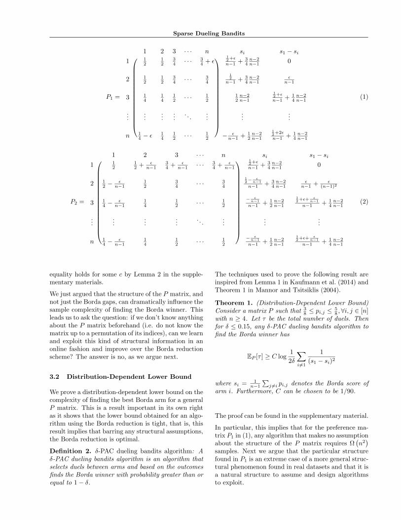
The matrices P1 and P2 above illustrate a key struc-tural aspect that can make it easier to find the Bordawinner. If the arms with the top Borda scores are dis-tinguished by duels with a small subset of the arms (asexemplified in P1), then finding the Borda winner maybe easier than in the general case. Before formalizinga model for this sort of structure, let us look at tworeal-world datasets, which motivate the model.

We consider the Microsoft Learning to Rank websearch datasets MSLR-WEB10k (Qin et al., 2010) andMQ2008-list (Qin and Liu, 2013) (see the experimen-tal section for a descrptions). Each dataset is used toconstruct a corresponding probability matrix P . Weuse these datasets to test the hypothesis that com-parisons with a small subset of the arms may sufficeto determine which of two arms has a greater Bordascore.

Specifically, we will consider the Borda score of thebest arm (arm 1) and every other arm. For any otherarm i > 1 and any positive integer k ∈ [n − 2], letΩi,k be a set of cardinality k containing the indicesj ∈ [n] \ 1, i with the k largest discrepancies |p1,j −pi,j |. These are the duels that, individually, displaythe greatest differences between arm 1 and i. For eachk, define αi(k) = 2(p1,i − 1

2 ) +∑j∈Ωi,k

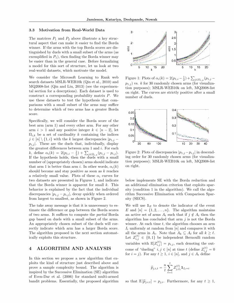
(p1,j − pi,j).If the hypothesis holds, then the duels with a smallnumber of (appropriately chosen) arms should indicatethat arm 1 is better than arm i. In other words, αi(k)should become and stay positive as soon as k reachesa relatively small value. Plots of these αi curves fortwo datasets are presented in Figures 1, and indicatethat the Borda winner is apparent for small k. Thisbehavior is explained by the fact that the individualdiscrepancies |p1,j − pi,j |, decay quickly when orderedfrom largest to smallest, as shown in Figure 2.

The take away message is that it is unnecessary to es-timate the difference or gap between the Borda scoresof two arms. It suffices to compute the partial Bordagap based on duels with a small subset of the arms.An appropriately chosen subset of the duels will cor-rectly indicate which arm has a larger Borda score.The algorithm proposed in the next section automat-ically exploits this structure.

4 ALGORITHM AND ANALYSIS

In this section we propose a new algorithm that ex-ploits the kind of structure just described above andprove a sample complexity bound. The algorithm isinspired by the Successive Elimination (SE) algorithmof Even-Dar et al. (2006) for standard multi-armedbandit problems. Essentially, the proposed algorithm

Figure 1: Plots of αi(k) = 2(p1,i− 12 ) +

∑j∈Ωi,k

(p1,j−p1,j) vs. k for 30 randomly chosen arms (for visualiza-tion purposes); MSLR-WEB10k on left, MQ2008-liston right. The curves are strictly positive after a smallnumber of duels.

Figure 2: Plots of discrepancies |p1,j−pi,j | in descend-ing order for 30 randomly chosen arms (for visualiza-tion purposes); MSLR-WEB10k on left, MQ2008-liston right.

below implements SE with the Borda reduction andan additional elimination criterion that exploits spar-sity (condition 1 in the algorithm). We call the algo-rithm Successive Elimination with Comparison Spar-sity (SECS).

We will use 1E to denote the indicator of the eventE and [n] = 1, 2, . . . , n. The algorithm maintainsan active set of arms At such that if j /∈ At then thealgorithm has concluded that arm j is not the Bordawinner. At each time t, the algorithm chooses an armIt uniformly at random from [n] and compares it withall the arms in At. Note that Ak ⊆ A` for all k ≥ `.Let Z

(t)i,j ∈ 0, 1 be independent Bernoulli random

variables with E[Z(t)i,j ] = pi,j , each denoting the out-

come of “dueling” i, j ∈ [n] at time t (define Z(t)i,j = 0

for i = j). For any t ≥ 1, i ∈ [n], and j ∈ At define

pj,i,t =n

t

t∑`=1

Z(`)j,I`

1I`=i

so that E [pj,i,t] = pj,i. Furthermore, for any t ≥ 1,

Sparse Dueling Bandits

Algorithm 1: Sparse Borda Algorithm

Input sparsity level k ∈ [n− 2], time gate T0 ≥ 0Start with active set A1 = 1, 2, · · · , n, t = 1

Let Ct =√

2 log(4n2t2/δ)t/n + 2 log(4n2t2/δ)

3t/n

while |At| > 1 doChoose It uniformly at random [n].for j ∈ At do

Observe Z(t)j,It

and update pj,It,t = nt

∑t`=1 Z

(`)j,I`

1I`=It , sj,t = n/(n−1)t

∑t`=1 Z

(`)j,I`

.

end

At+1 = At \j ∈ At : ∃i ∈ At with

1) 1t>T0 ∆i,j,t

(arg maxΩ⊂[n]:|Ω|=k ∇i,j,t(Ω)

)> 6(k + 1)Ct

OR 2) si,t > sj,t + nn−1

√2 log(4nt2/δ)

t

t← t+ 1

end

j ∈ At define

sj,t =n/(n− 1)

t

t∑`=1

Z(`)j,I`

so that E [sj,t] = sj . For any Ω ⊂ [n] and i, j ∈ [n]define

∆i,j(Ω) = 2(pi,j − 12 ) +

∑ω∈Ω:ω 6=i 6=j

(pi,ω − pj,ω)

∆i,j,t(Ω) = 2(pi,j,t − 12 ) +

∑ω∈Ω:ω 6=i 6=j

(pi,ω,t − pj,ω,t)

∇i,j(Ω) =∑

ω∈Ω:ω 6=i 6=j

|pi,ω − pj,ω|

∇i,j(Ω) =∑

ω∈Ω:ω 6=i 6=j

|pi,ω,t − pj,ω,t| .

The quantity ∆i,j(Ω) is the partial gap between theBorda scores for i and j, based on only the comparisonswith the arms in Ω. Note that 1

n−1∆i,j([n]) = si −sj . The quantity arg maxΩ⊂[n]:|Ω|=k∇i,j(Ω) selects theindices ω yielding the largest discrepancies |pi,ω−pj,ω|.∆ and ∇ are empirical analogs of these quantities.

Definition 3. For any i ∈ [n] \ 1 we say the set(p1,ω − pi,ω)ω 6=16=i is (γ, k)-approximately sparse if

maxΩ∈[n]:|Ω|≤k

∇1,i(Ω \ Ωi) ≤ γ∆1,i(Ωi)

where Ωi = arg maxΩ⊂[n]:|Ω|=k

∇1,i(Ω).

Instead of the strong assumption that the set (p1,ω −pi,ω)ω 6=16=i has no more than k non-zero coefficients,the above definition relaxes this idea and just assumesthat the absolute value of the coefficients outside the

largest k are small relative to the partial Borda gap.This definition is inspired by the structure describedin previous sections and will allow us to find the Bordawinner faster.

The parameter T0 is specified (see Theorem 2) to guar-antee that all arms with sufficiently large gaps s1 − siare eliminated by time step T0 (condition 2). Oncet > T0, condition 1 also becomes active and the algo-rithm starts removing arms with large partial Bordagaps, exploiting the assumption that the top arms canbe distinguished by comparisons with a sparse set ofother arms. The algorithm terminates when only onearm remains.

Theorem 2. Let k ≥ 0 and T0 > 0 be inputsto the above algorithm and let R be the solution to32R2 log

(32n/δR2

)= T0. If for all i ∈ [n] \ 1, at least one

of the following holds:

1. (p1,ω − pi,ω)ω 6=16=i is ( 13 , k)-approximately

sparse,

2. (s1 − si) ≥ R,

then with probability at least 1− 3δ, the algorithm re-turns the best arm after no more than

c∑j>1

min

max

1R2 log

(n/δR2

), (k+1)2/n

∆2j

log(n/δ∆2j

),

1∆2j

log(n/δ∆2j

)samples where ∆j := s1 − sj and c > 0 is an absoluteconstant.

The second argument of the min is precisely the re-sult one would obtain by running Successive Elimina-tion with the Borda reduction (Even-Dar et al., 2006).

Jamieson, Katariya, Deshpande, Nowak

Thus, under the stated assumptions, the algorithmnever does worse than the Borda reduction scheme.The first argument of the min indicates the poten-tial improvement gained by exploiting the sparsity as-sumption. The first argument of the max is the resultof throwing out the arms with large Borda differencesand the second argument is the result of throwing outarms where a partial Borda difference was observed tobe large.

To illustrate the potential improvements, consider theP1 matrix discussed above, the theorem implies that

by setting T0 = 32R2 log

(32n/δR2

)with R = 1/2+ε

n−1 +14n−2n−1 ≈

14 and k = 1 we obtain a sample complexity of

O(ε−2n log(n)) for the proposed algorithm comparedto the standard Borda reduction sample complexity ofΩ(n2).

In practice it is difficult optimize the choice of T0 andk, but motivated by the results shown in the experi-ments section, we recommend setting T0 = 0 and k = 5for typical problems.

5 EXPERIMENTS

The goal of this section is not to obtain the bestpossible sample complexity results for the specifieddatasets, but to show the relative performance gainof exploiting structure using the proposed SECS algo-rithm with respect to the Borda reduction. That is, wejust want to measure the effect of exploiting sparsitywhile keeping all other parts of the algorithms con-stant. Thus, the algorithm we compare to that uses thesimple Borda reduction is simply the SECS algorithmdescribed above but with T0 = ∞ so that the sparsecondition never becomes activated. Running the al-gorithm in this way, it is very closely related to theSuccessive Elimination algorithm of Even-Dar et al.(2006). In what follows, our proposed algorithm willbe called SECS and the benchmark algorithm will bedenoted as just the Borda reduction (BR) algorithm.

We experiment on both simulated data and two real-world datasets. During all experiments, both the BRand SECS algorithms were run with δ = 0.1. For theSECS algorithm we set T0 = 0 to enable condition 1from the very beginning (recall for BR we set T0 =∞). Also, while the algorithm has a constant factorof 6 multiplying (k + 1)Ct, we feel that the analysisthat led to this constant is very loose so in practicewe recommend the use of a constant of 1/2 which wasused in our experiments. While the change of thisconstant invalidates the guarantee of Theorem 2, wenote that in all of the experiments to be presentedhere, neither algorithm ever failed to return the bestarm. This observation also suggests that the SECS

Figure 3: Comparison of the Borda reduction algo-rithm and the proposed SECS algorithm ran on theP1 matrix for different values of n. Plot is on log-log scale so that the sample complexity grows like ns

where s is the slope of the line.

algorithm is robust to possible inconsistencies of themodel assumptions.

5.1 Synthetic Preference matrix

Both algorithms were tasked with finding the best armusing the P1 matrix of (1) with ε = 1/5 for problemsizes equal to n = 10, 20, 30, 40, 50, 60, 70, 80 arms. In-specting the P1 matrix, we see that a value of k = 1 inthe SECS algorithm suffices so this is used for all prob-lem sizes. The entries of the preference matrix Pi,j areused to simulate comparisons between the respectivearms and each experiment was repeated 75 times.

Recall from Section 3 that any algorithm using theBorda reduction on the P1 matrix has a sample com-plexity of Ω(n2). Moreover, inspecting the proof ofTheorem 2 one concludes that the BR algorithm has asample complexity of O(n2 log(n)) for the P1 matrix.On the other hand, Theorem 2 states that the SECSalgorithm should have a sample complexity no worsethan O(n log(n)) for the P1 matrix. Figure 3 plotsthe sample complexities of SECS and BR on a log-logplot. On this scale, to match our sample complexityhypotheses, the slope of the BR line should be about2 while the slope of the SECS line should be about 1,which is exactly what we observe.

5.2 Web search data

We consider two web search data sets. The first isthe MSLR-WEB10k Microsoft Learning to Rank dataset (Qin et al., 2010) that is characterized by approx-imately 30,000 search queries over a number of docu-

Sparse Dueling Bandits

ments from search results. The data also contains thevalues of 136 features and corresponding user labelledrelevance factors with respect to each query-documentpair. We use the training set of Fold 1, which com-prises of about 2,000 queries. The second data set isthe MQ2008-list from the Microsoft Learning to Rank4.0 (MQ2008) data set (Qin and Liu, 2013). We usethe training set of Fold 1, which has about 550 queries.Each query has a list of documents with 46 featuresand corresponding user labelled relevance factors.

For each data set, we create a set of rankers, each corre-sponding to a feature from the feature list. The aim ofthis task is be to determine the feature whose rankingof query-document pairs is the most relevant. To com-pare two rankers, we randomly choose a pair of docu-ments and compare their relevance rankings with thoseof the features. Whenever a mismatch occurs betweenthe rankings returned by the two features, the featurewhose ranking matches that of the relevance factors ofthe two documents “wins the duel”. If both featuresrank the documents similarly, the duel is deemed tohave resulted in a tie and we flip a fair coin. We run aMonte Carlo simulation on both data sets to obtain apreference matrix P corresponding to their respectivefeature sets. As with the previous setup, the entriesof the preference matrices ([P ]i,j = pi,j) are used tosimulate comparisons between the respective arms andeach experiment was repeated 75 times.

From the MSLR-WEB10k data set, a single arm wasremoved for our experiments as its Borda score wasunreasonably close to the arm with the best Bordascore and behaved unlike any other arm in the datasetwith respect to its αi curves, confounding our model.For these real datasets, we consider a range of differ-ent k values for the SECS algorithm. As noted above,while there is no guarantee that the SECS algorithmwill return the true Borda winner, in all of our trialsfor all values of k reported we never observed a singleerror. This is remarkable as it shows that the correct-ness of the algorithm is insensitive to the value of k onat least these two real datasets. The sample complex-ities of BR and SECS on both datasets are reportedin Figure 4. We observe that the SECS algorithm, forsmall values of k, can identify the Borda winner usingas few as half the number required using the Borda re-duction method. As k grows, the performance of theSECS algorithm becomes that of the BR algorithm, aspredicted by Theorem 2.

Lastly, the preference matrices of the two data setssupport the argument for finding the Borda winnerover the Condorcet winner. The MSLR-WEB10k dataset has no Condorcet winner arm. However, while theMQ2008 data set has a Condorcet winner, when weconsider the Borda scores of the arms, it ranks second.

(a) MSLR-WEB10k (b) MQ2008

Figure 4: Comparison of an action elimination-stylealgorithm using the Borda reduction (denoted as BR)and the proposed SECS algorithm with different valuesof k on the two datasets.

Jamieson, Katariya, Deshpande, Nowak

References

Ailon, N., Joachims, T., and Karnin, Z. (2014). Re-ducing dueling bandits to cardinal bandits. arXivpreprint arXiv:1405.3396.

Boucheron, S., Lugosi, G., and Massart, P. (2013).Concentration inequalities: A nonasymptotic theoryof independence. Oxford University Press.

Even-Dar, E., Mannor, S., and Mansour, Y. (2006).Action elimination and stopping conditions forthe multi-armed bandit and reinforcement learningproblems. The Journal of Machine Learning Re-search, 7:1079–1105.

Jamieson, K., Malloy, M., Nowak, R., and Bubeck, S.(2014). lil’ucb : An optimal exploration algorithmfor multi-armed bandits. COLT.

Karnin, Z., Koren, T., and Somekh, O. (2013). Al-most optimal exploration in multi-armed bandits.In Proceedings of the 30th International Conferenceon Machine Learning.

Kaufmann, E., Cappe, O., and Garivier, A. (2014).On the complexity of best arm identificationin multi-armed bandit models. arXiv preprintarXiv:1407.4443.

Mannor, S. and Tsitsiklis, J. N. (2004). The samplecomplexity of exploration in the multi-armed ban-dit problem. The Journal of Machine Learning Re-search, 5:623–648.

Qin, T. and Liu, T.-Y. (2013). Introducing letor 4.0datasets. CoRR, abs/1306.2597.

Qin, T., Liu, T.-Y., Xu, J., and Li, H. (2010). Letor:A benchmark collection for research on learningto rank for information retrieval. Information Re-trieval, 13(4):346–374.

Urvoy, T., Clerot, F., Feraud, R., and Naamane, S.(2013). Generic exploration and k-armed votingbandits. In Proceedings of the 30th InternationalConference on Machine Learning (ICML-13), pages91–99.

Yue, Y., Broder, J., Kleinberg, R., and Joachims, T.(2012). The k-armed dueling bandits problem. Jour-nal of Computer and System Sciences, 78(5):1538–1556.

Yue, Y. and Joachims, T. (2011). Beat the mean ban-dit. In Proceedings of the 28th International Confer-ence on Machine Learning (ICML-11), pages 241–248.

Zoghi, M., Whiteson, S., Munos, R., and de Rijke,M. (2013). Relative upper confidence bound forthe k-armed dueling bandit problem. arXiv preprintarXiv:1312.3393.

Sparse Dueling Bandits

A Proof of Lower Bound

We begin by stating a few technical lemmas. At the heart of the proof of the lower bound is Lemma 1 ofKaufmann et al. (2014) restated here for completeness.

Lemma 1. Let ν and ν′ be two bandit models defined over n arms. Let σ be a stopping time with respect to (Ft)and let A ∈ Fσ be an event such that 0 < Pν(A) < 1. Then

n∑a=1

Eν [Na(σ)]KL(νa, ν′a) ≥ d(Pν(A),Pν′(A))

where d(x, y) = x log(x/y) + (1− x) log((1− x)/(1− y)).

Note that the function d is exactly the KL-divergence between two Bernoulli distributions.

Corollary 1. Let Ni,j = Nj,i denote the number of duels between arms i and j. For the duelling bandits problem

with n arms, we have (n−1)(n−2)2 free parameters (or arms). These are the numbers in the upper triangle of the

P matrix. Then, if P ′ is an alternate matrix, we have from Lemma 1,

n∑i=1

n∑j=i+1

EP [Ni,j ]d(pi,j , p′i,j) ≥ d(PP (A),PP ′(A))

The above corollary relates the cumulative number of duels of a subset of arms to the uncertainty between theactual distribution and an alternative distribution. In deference to interpretability rather than preciseness, wewill use the following bound of the KL divergence.

Lemma 2. (Upper bound on KL Divergence for Bernoullis) Consider two Bernoulli random variables with meansp and q, 0 < p, q < 1. Then

d(p, q) ≤ (p− q)2

q(1− q)

Proof.

d(p, q) = p logp

q+ (1− p) log

1− p1− q

≤ pp− qq

+ (1− p)q − p1− q

=(p− q)2

q(1− q)

where we use the fact that log x ≤ x− 1 for x > 0.

We are now in a position to restate and prove the lower bound theorem.

Theorem 3. (Lower bound on sample complexity of finding Borda winner for the Dueling Bandits Problem)Consider a matrix P such that 3

8 ≤ pi,j ≤ 58 ,∀i, j ∈ [n], and n ≥ 3. Then for δ ≤ 0.15, any δ-PAC dueling

bandits algorithm to find the Borda winner has

EP [τ ] ≥ C(n− 2

n− 1

)2∑i 6=1

1

(s1 − si)2

log1

2δ

where si = 1n−1

∑j 6=i

pi,j denotes the Borda score of arm i. C can be chosen to be 140 .

Proof. Consider an alternate hypothesis P ′ where arm b is the best arm, and such that P ′ differs from P onlyin the indices bj : j /∈ 1, b. Note that the Borda score of arm 1 is unaffected in the alternate hypothesis.Corollary 1 then gives us: ∑

j∈[n]\1,b

EP [Nb,j ]d(pb,j , p′b,j) ≥ d(P(A),P(A′)) (3)

Let A be the event that the algorithm selects arm 1 as the best arm. Since we assume a δ-PAC algorithm,PP (A) ≥ 1− δ, PP ′(A) ≤ δ. It can be shown that for δ ≤ 0.15, d(PP (A),PP ′(A)) ≥ log 1

2δ .

Jamieson, Katariya, Deshpande, Nowak

Define Nb =∑j 6=b

Nb,j . Consider

(maxj /∈1,b

(pb,j − p′b,j)2

p′b,j(1− p′b,j)

)EP [Nb] ≥

(maxj /∈1,b

d(pb,j , p′b,j)

)EP [Nb]

=

(maxj /∈1,b

d(pb,j , p′b,j)

)∑j 6=b

EP [Nb,j ]

≥(

maxj /∈1,b

d(pb,j , p′b,j)

) ∑j /∈1,b

EP [Nb,j ]

≥

∑j∈[n]\1,b

EP [Nb,j ]d(pb,j , p′b,j)

≥ log1

2δ. (by (3)) (4)

In particular, choose p′b,j = pb,j + n−1n−2 (s1 − sb) + ε, j /∈ 1, b. As required, under hypothesis P ′, arm b is the

best arm.

Since pb,j ≤ 58 , s1 ≤ 5

8 , and sb ≥ 38 , as ε 0, lim

ε0p′b,j ≤ 15

16 . This implies 1p′b,j(1−p

′b,j)≤ 256

15 ≤ 20. (4) implies

20

(n− 1

n− 2(s1 − sb) + ε

)2

EP [Nb] ≥ log1

2δ

⇒ EP [Nb] ≥1

20

(n− 2

n− 1

)21

(s1 − sb)2log

1

2δ(5)

where we let ε 0.

Finally, iterating over all arms b 6= 1, we have

EP [τ ] =1

2

n∑b=1

∑j 6=b

EP [Nb,j ] =1

2

n∑b=1

EP [Nb] ≥1

2

n∑b=2

EP [Nb] ≥1

40

(n− 2

n− 1

)2∑b6=1

1

(s1 − sb)2

log1

2δ

B Proof of Upper Bound

To prove the theorem we first need a technical lemma.

Lemma 3. For all s ∈ N, let Is be drawn independently and uniformly at random from [n] and let Z(s)i,j be a

Bernoulli random variable with mean pi,j. If pi,j,t = nt

∑ts=1 Z

(s)i,j 1Is=j for all i ∈ [n] and Ct =

√2 log(4n2t2/δ)

t/n +

2 log(4n2t2/δ)3t/n then P

(⋃(i,j)∈[n]2:i6=j

⋃∞t=1 |pi,j,t − pi,j | > Ct

)≤ δ.

Proof. Note that tpi,j,t =∑ts=1 nZ

(s)i,j 1Is=j is a sum of i.i.d. random variables taking values in [0, n] with

E[(nZ

(s)i,j 1Is=j

)2]≤ n2E [1Is=j ] ≤ n. A direct application of Bernstein’s inequality (Boucheron et al., 2013)

and union bounding over all pairs (i, j) ∈ [n]2 and time t gives the result.

Sparse Dueling Bandits

A consequence of the lemma is that by repeated application of the triangle inequality,∣∣∣∇i,j,t(Ω)−∇i,j(Ω)∣∣∣ =

∣∣∣∣ ∑ω∈Ω:ω 6=i 6=j

|pi,ω,t − pj,ω,t| − |pi,ω − pj,ω|∣∣∣∣

≤∑

ω∈Ω:ω 6=i 6=j

|pi,ω,t − pi,ω|+ |pj,ω − pj,ω,t|

≤ 2|Ω|Ct

and similarly∣∣∣∆i,j,t(Ω)−∆i,j(Ω)

∣∣∣ ≤ 2(1 + |Ω|)Ct for all i, j ∈ [n] with i 6= j, all t ∈ N and all Ω ⊂ [n]. We are

now ready to prove Theorem 2.

Proof. We begin the proof by defining Ct(Ω) = 2(1 + |Ω|)Ct and considering the events

∞⋂t=1

⋂Ω⊂[n]

|∆i,j,t(Ω)−∆i,j(Ω)| < Ct(Ω)

,

∞⋂t=1

⋂Ω⊂[n]

|∇i,j,t(Ω)−∇i,j(Ω)| < Ct(Ω)

,

∞⋂t=1

n⋂i=1

|si,t − si| <

n

n− 1

√log(4nt2/δ)

2t

,

that each hold with probability at least 1− δ. The first set of events are a consequence of Lemma 3 and the lastset of events are proved using a straightforward Hoeffding bound (Boucheron et al., 2013) and a union boundsimilar to that in Lemma 3. In what follows assume these events hold.

Step 1: If t > T0 and s1 − sj > R, then j /∈ At.We begin by considering all those j ∈ [n] \ 1 such that s1 − sj ≥ R and show that with the prescribed value ofT0, these arms are thrown out before t > T0. By the events defined above, for arbitrary i ∈ [n] \ 1 we have

si,t − s1,t = si,t − si + s1 − s1,t + si − s1 ≤ si − s1 +2n

n− 1

√log(4nt2/δ)

2t≤ 2n

n− 1

√log(4nt2/δ)

2t

since by definition s1 > si. This proves that the best arm will never be thrown out using the Borda reductionwhich implies that 1 ∈ At for all t ≤ T0. On the other hand, for any j ∈ [n] \ 1 such that s1− sj ≥ R and t ≤ T0

we have

maxi∈At

si,t − sj,t ≥ s1,t − sj,t

≥ s1 − sj −2n

n− 1

√log(4nt2/δ)

2t

=∆1,j([n])

n− 1− 2n

n− 1

√log(4nt2/δ)

2t.

If τj is the first time t that the right hand side of the above is greater than or equal to 2nn−1

√log(4nt2/δ)

2t then

τj ≤32n2

∆21,j([n])

log

(32n3/δ

∆21,j([n])

),

since for all positive a, b, t with a/b ≥ e we have t ≥ 2 log(a/b)b =⇒ b ≥ log(at)

t . Thus, any j with∆1,j([n])n−1 = s1 − sj ≥ R has τj ≤ T0 which implies that any i ∈ At for t > T0 has s1 − si ≤ R.

Step 2: For all t, 1 ∈ At.We showed above that the Borda reduction will never remove the best arm from At. We now show that the

Jamieson, Katariya, Deshpande, Nowak

sparse-structured discard condition will not remove the best arm. At any time t > T0, let i ∈ [n] \ 1 be arbitrary

and let Ωi = arg maxΩ⊂[n]:|Ω|=k

∇i,1,t(Ω) and Ωi = arg maxΩ⊂[n]:|Ω|=k

∇i,1(Ω). Note that for any Ω ⊂ [n] we have

∇i,1(Ω) = ∇1,i(Ω) but ∆i,1(Ω) = −∆1,i(Ω) and

∆i,1,t(Ωi) ≤ ∆i,1(Ωi) + Ct(Ωi)

= ∆i,1(Ωi)−∆i,1(Ωi) + ∆i,1(Ωi) + Ct(Ωi)

=

∑ω∈Ωi

(pi,ω − p1,ω)

−(∑ω∈Ωi

(pi,ω − p1,ω)

)−∆1,i(Ωi) + Ct(Ωi)

≤ −

∑ω∈Ωi\Ωi

(pi,ω − p1,ω)

− 2

3∆1,i(Ωi) + Ct(Ωi)

since(∑

ω∈Ωi\Ωi(pi,ω − p1,ω))≤ ∇1,i

(Ωi \ Ωi

)≤ 1

3∆1,i(Ωi) by the conditions of the theorem. Continuing,

∆i,1,t(Ωi) ≤ −

∑ω∈Ωi\Ωi

(pi,ω − p1,ω)

− 2

3∆1,i(Ωi) + Ct(Ωi)

≤

∑ω∈Ωi\Ωi

|pi,ω,t − p1,ω,t|

− 2

3∆1,i(Ωi) + Ct(Ωi) + Ct(Ωi \ Ωi)

≤

∑ω∈Ωi\Ωi

|pi,ω,t − p1,ω,t|

− 2

3∆1,i(Ωi) + Ct(Ωi) + Ct(Ωi \ Ωi)

≤

∑ω∈Ωi\Ωi

|pi,ω − p1,ω|

− 2

3∆1,i(Ωi) + Ct(Ωi) + Ct(Ωi \ Ωi) + Ct(Ωi \ Ωi)

≤ −1

3∆1,i(Ωi) + Ct(Ωi) + Ct(Ωi \ Ωi) + Ct(Ωi \ Ωi)

≤ 3 maxΩ⊂[n]:|Ω|≤k

Ct(Ω) = 6(1 + k)Ct

where the third inequality follows from the fact that ∇i,1,t(

Ωi \ Ωi

)≤ ∇i,1,t

(Ωi \ Ωi

)by definition, and the

second-to-last line follows again by the same theorem condition used above. Thus, combining both steps oneand two, we have that 1 ∈ At for all t.

Step 3 : Sample ComplexityAt any time t > T0, let j ∈ [n] \ 1 be arbitrary and let Ωi = arg max

Ω⊂[n]:|Ω|=k∇1,j,t(Ω) and Ωi =

Sparse Dueling Bandits

arg maxΩ⊂[n]:|Ω|=k

∇1,j(Ω). We begin with

maxi∈[n]\j

∆i,j,t

(Ωi

)≥ ∆1,j,t(Ωi)

≥ ∆1,j(Ωi)− Ct(Ωi)

≥ ∆1,j(Ωi)−∆1,j(Ωi) + ∆1,j(Ωi)− Ct(Ωi)

=

∑ω∈Ω

(p1,ω − pj,ω)

−(∑ω∈Ωi

(p1,ω − pj,ω)

)+ ∆1,j(Ωi)− Ct(Ωi)

≥ −

∑ω∈Ωi\Ω

(pi,ω − p1,ω)

+2

3∆1,j(Ωi)− Ct(Ωi)

≥ −

∑ω∈Ωi\Ω

|pi,ω,t − p1,ω,t|

+2

3∆1,j(Ωi)− Ct(Ωi)− Ct(Ωi \ Ωi)

≥ −

∑ω∈Ωi\Ωi

|pi,ω,t − p1,ω,t|

+2

3∆1,j(Ωi)− Ct(Ωi)− Ct(Ωi \ Ωi)

≥ −

∑ω∈Ωi\Ωi

|pi,ω − p1,ω|

+2

3∆1,j(Ωi)− Ct(Ωi)− Ct(Ωi \ Ωi)− Ct(Ωi \ Ωi)

≥ 1

3∆1,j(Ωi)− 3 max

Ω⊂[n]:|Ω|≤kCt(Ω) =

1

3∆1,j(Ωi)− 6(1 + k)Ct

by a series of steps as analogous to those in Step 2. If τj is the first time t > T0 such that the right hand side isgreater than or equal to 6(1 + k)Ct, the point at which j would be removed, we have that

τj ≤20736n(k + 1)2

∆21,j(Ωi)

log

(20736n2(k + 1)2

∆21,j(Ωi) δ

)

using the same inequality as above in Step 2. Combining steps one and three we have that the total number ofsamples taken is bounded by

∑j>1

min

max

T0,

20736n(k + 1)2

∆21,j(Ωi)

log

(20736n2(k + 1)2

∆21,j(Ωi) δ

),

32n2

∆21,j([n])

log

(32n3/δ

∆21,j([n])

)

with probability at least 1 − 3δ. The result follows from recalling that∆1,j(Ωi)n−1 = s1 − sj and noticing that

nn−1 ≤ 2 for n ≥ 2.