PONTIFICIA UNIVERSIDAD CATOLICA DE CHILE

SCHOOL OF ENGINEERING

SPARSE KNN – A METHOD FOR OBJECT

RECOGNITION OVER X-RAY IMAGES

USING KNN BASED IN SPARSE

RECONSTRUCTION

ERICK SVEC P.

Thesis submitted to the Office of Research and Graduate Studies

in partial fulfillment of the requirements for the degree of

Master of Science in Engineering

Advisor:

DOMINGO MERY QUIROZ

Santiago de Chile, August 2016

c©MMXV, ERICK VACLAV SVEC PARRA

PONTIFICIA UNIVERSIDAD CATOLICA DE CHILE

SCHOOL OF ENGINEERING

SPARSE KNN – A METHOD FOR OBJECT

RECOGNITION OVER X-RAY IMAGES

USING KNN BASED IN SPARSE

RECONSTRUCTION

ERICK SVEC P.

Members of the Committee:

DOMINGO MERY QUIROZ

KARIM PICHARA BAKSAI

SERGIO HERNANDEZ ALVAREZ

CRISTIAN ANDRES TEJOS NUNEZ

Thesis submitted to the Office of Research and Graduate Studies

in partial fulfillment of the requirements for the degree of

Master of Science in Engineering

Santiago de Chile, August 2016

To my Mother, Father and Sisters,

for encouraging me and their

unconditional support

ACKNOWLEDGEMENTS

First of all, I want to show gratitude to my parents: Wenceslao and Alicia Svec in

addition to my sisters Katiushka and Valeshka Svec for walking this path by my side al-

ways with loving support. With appreciation, I share my gratitude to Domingo Mery who

taught me not only of computer vision, but has been a true companion and guide during my

learning period and thesis development. I also wish to give thanks to Tomas Larrain and

Marco Arias for numberless conversations and ideas while we develop our thesis. Finally,

thanks to Rocio Escobedo for her support during this last period.

”Now ye may suppose that this is foolishness in me; but behold I say unto

you, that by small and simple things are great things brought to pass; and

small means in many instances doth confound the wise.”

—ALMA, About 74 B.C.

iv

TABLE OF CONTENTS

ACKNOWLEDGEMENTS . . . . . . . . . . . . . . . . . . . . . . . . . . . . . iv

LIST OF FIGURES . . . . . . . . . . . . . . . . . . . . . . . . . . . . . . . . . vii

LIST OF TABLES . . . . . . . . . . . . . . . . . . . . . . . . . . . . . . . . . . ix

ABSTRACT . . . . . . . . . . . . . . . . . . . . . . . . . . . . . . . . . . . . . x

RESUMEN . . . . . . . . . . . . . . . . . . . . . . . . . . . . . . . . . . . . . xi

1. INTRODUCCION . . . . . . . . . . . . . . . . . . . . . . . . . . . . . . . 1

1.1. The problem . . . . . . . . . . . . . . . . . . . . . . . . . . . . . . . . 1

1.2. State of the Art . . . . . . . . . . . . . . . . . . . . . . . . . . . . . . . 2

1.3. Motivation . . . . . . . . . . . . . . . . . . . . . . . . . . . . . . . . . 4

1.4. Known Methods . . . . . . . . . . . . . . . . . . . . . . . . . . . . . . 5

1.4.1. k-Nearest Neighbors (knn) . . . . . . . . . . . . . . . . . . . . . . . 5

1.4.2. Sequential Fordward Selection (SFS) . . . . . . . . . . . . . . . . . 6

1.4.3. SIFT . . . . . . . . . . . . . . . . . . . . . . . . . . . . . . . . . . 7

1.4.4. K-means . . . . . . . . . . . . . . . . . . . . . . . . . . . . . . . . 8

1.4.5. Sparse Reconstruction . . . . . . . . . . . . . . . . . . . . . . . . . 9

2. PROPOSED METHOD . . . . . . . . . . . . . . . . . . . . . . . . . . . . . 11

2.1. Training . . . . . . . . . . . . . . . . . . . . . . . . . . . . . . . . . . . 12

2.1.1. Feature Extraction . . . . . . . . . . . . . . . . . . . . . . . . . . . 12

2.1.2. Delta Feature . . . . . . . . . . . . . . . . . . . . . . . . . . . . . . 13

2.1.3. SFS . . . . . . . . . . . . . . . . . . . . . . . . . . . . . . . . . . . 14

2.1.4. Kmeans . . . . . . . . . . . . . . . . . . . . . . . . . . . . . . . . 16

2.1.5. Dictionary Construction . . . . . . . . . . . . . . . . . . . . . . . . 17

2.2. Testing . . . . . . . . . . . . . . . . . . . . . . . . . . . . . . . . . . . 17

2.2.1. Feature Extraction . . . . . . . . . . . . . . . . . . . . . . . . . . . 18

v

2.2.2. Classifiers . . . . . . . . . . . . . . . . . . . . . . . . . . . . . . . 18

2.2.3. SoftVoting . . . . . . . . . . . . . . . . . . . . . . . . . . . . . . . 21

3. Experiments and Restults . . . . . . . . . . . . . . . . . . . . . . . . . . . . 23

3.1. DataBase . . . . . . . . . . . . . . . . . . . . . . . . . . . . . . . . . . 23

3.1.1. Training Images . . . . . . . . . . . . . . . . . . . . . . . . . . . . 23

3.1.2. Testing Images . . . . . . . . . . . . . . . . . . . . . . . . . . . . . 24

3.2. Experiments . . . . . . . . . . . . . . . . . . . . . . . . . . . . . . . . 26

3.2.1. Parameters adjustment . . . . . . . . . . . . . . . . . . . . . . . . . 26

3.3. Curves . . . . . . . . . . . . . . . . . . . . . . . . . . . . . . . . . . . 31

3.4. Results . . . . . . . . . . . . . . . . . . . . . . . . . . . . . . . . . . . 35

3.4.1. Validation Performance . . . . . . . . . . . . . . . . . . . . . . . . 35

3.4.2. Comparison of different methods . . . . . . . . . . . . . . . . . . . 36

4. CONCLUSION . . . . . . . . . . . . . . . . . . . . . . . . . . . . . . . . . 39

References . . . . . . . . . . . . . . . . . . . . . . . . . . . . . . . . . . . . . . 41

vi

LIST OF FIGURES

1.1 Knn Classification . . . . . . . . . . . . . . . . . . . . . . . . . . . . . . . . 6

1.2 K-means Clustering . . . . . . . . . . . . . . . . . . . . . . . . . . . . . . . 8

2.1 Method Overview . . . . . . . . . . . . . . . . . . . . . . . . . . . . . . . . 11

2.2 Training Diagram . . . . . . . . . . . . . . . . . . . . . . . . . . . . . . . . 12

2.3 Morphological Procesing Example . . . . . . . . . . . . . . . . . . . . . . . 13

2.4 Representation of what the δ feature represents . . . . . . . . . . . . . . . . . 14

2.5 SIFT visual representation in a Shuriken Image . . . . . . . . . . . . . . . . . 15

2.6 Normalized sift gradient representation . . . . . . . . . . . . . . . . . . . . . 16

2.7 Abundant similar keypoints in the same object . . . . . . . . . . . . . . . . . . 16

2.8 Testing Diagram . . . . . . . . . . . . . . . . . . . . . . . . . . . . . . . . . 17

2.9 Visualization of feature selection . . . . . . . . . . . . . . . . . . . . . . . . 19

2.10Example SCI threshold . . . . . . . . . . . . . . . . . . . . . . . . . . . . . 20

3.1 Example of training set . . . . . . . . . . . . . . . . . . . . . . . . . . . . . 24

3.2 A gun rotating as an example of rotation of the objects . . . . . . . . . . . . . 24

3.3 Example of testing images . . . . . . . . . . . . . . . . . . . . . . . . . . . . 25

3.4 Example of testing Set . . . . . . . . . . . . . . . . . . . . . . . . . . . . . . 25

3.5 Jmax vs number of features for SFS . . . . . . . . . . . . . . . . . . . . . . . 27

3.6 Clean process of noisy keypoints . . . . . . . . . . . . . . . . . . . . . . . . 28

3.7 Accuracy Vs DistanceTresholdPistol . . . . . . . . . . . . . . . . . . . . . . 29

3.8 Accuracy Vs DistanceTresholdRazor . . . . . . . . . . . . . . . . . . . . . . 30

3.9 Accuracy Vs DistanceTresholdShuriken . . . . . . . . . . . . . . . . . . . . . 30

3.10Accuracy Vs minMaxDistance . . . . . . . . . . . . . . . . . . . . . . . . . . 31

3.11Precision-Recall Curves variating SCI parameter . . . . . . . . . . . . . . . . 32

vii

3.12Precision-Recall Curves variating distanceTresholdP istol parameter . . . . . 33

3.13Precision-Recall Curves variating distanceTresholdShuriken parameter . . . 33

3.14Precision-Recall Curves variating distanceTresholdRazor parameter . . . . . 34

3.15Precision-Recall Curves variating minMaxDistance parameter . . . . . . . . 35

3.16Confusion Matrix . . . . . . . . . . . . . . . . . . . . . . . . . . . . . . . . 38

viii

LIST OF TABLES

3.1 Distribution of images among all sets . . . . . . . . . . . . . . . . . . . . . . 26

3.2 Precision & Recall for validation set . . . . . . . . . . . . . . . . . . . . . . . 36

3.3 Accuracy for each detector in validation set (in percentages) in experiment (B) . 36

3.4 Precision & Recall for each detector . . . . . . . . . . . . . . . . . . . . . . . 37

3.5 Accuracy for each detector . . . . . . . . . . . . . . . . . . . . . . . . . . . . 37

ix

ABSTRACT

Object recognition in X rays images is not a trivial task. There is dealing with funda-

mental problems such as the absence of color or the particular occlusion inherent of this

problem, the second being different of what we are accustomed, inasmuch as in radiogra-

phy the object is always visible, as much as any other object present in the image at all

times, therefore, more than obstruct the image visibility, X-Rays combine them. It is for

this purpose we introduce a method based on SIFT keypoints extracted from the image.

These keypoints are first to be used to train a model for each present class, even Pistol,

Shuriken, Razor and Others or No-class. Then, using this model, we calculate the sparse

reconstruction of these keypoints, these are then classified by a metric distance, training

a different classifier for each class. A key stage of our method is feature selection, we

select around 50 features of the 128 SIFT keypoints features, being this selection differ-

ent for each classifier. The purpose for this selection is to diminish the added noise of

the radiologic occlusion before mentioned. It is empirically proved the parameters tunings

importance, which take a great importance by raising the algorithms performance, among

these tuning parameters are found, acceptance distances threshold, Sparsity Concentration

Index threshold, being this an index used to know if the sparse representation of one or

many classes; and a representation of the importance of the relative keypoint center of the

image position delta. The effectiveness of our method was tested in the recognition of

three different threat objects: pistols, shuriken (ninja stars) and razor blades. With above,

in our experiments, after parameter tuning, the highest recognition rate achieved is over

94% accuracy.

Keywords: sparse, rayos X, computer vision, object recognition, KNN, SCI, SIFT

x

RESUMEN

El reconocimiento de objetos en imagenes de rayos X no es una tarea trivial, lidiando

con problemas fundamentales tales como la ausencia de color o la oclusion particular del

problema, difiriendo esta segunda de la oclusion con la que generalmente nos encontramos,

puesto que en una radiografıa el objeto siempre es visible, ası como cada otro objeto en la

imagen, por lo que mas que obstruir la vision, las imagenes de rayos X las combinan. Es

por esto que se presenta un metodo basado en los puntos SIFT extraıdos de la imagen.

Estos puntos son primeramente usados para entrenar un modelo para cada clase presente,

Pistola, Shuriken, Hoja de afeitar y Otros o No clase. Luego, utilizando este modelo, se

busca la reconstruccion sparse de estos puntos, los cuales son clasificados utilizando una

metrica de distancia, construyendo un clasificador por cada clase. Una fase clave en este

metodo es la seleccion de caracterısticas, seleccionamos alrededor de 50 caracterısticas de

las 128 del descriptor SIFT, esta seleccion diferente para cada clasificador. La finalidad de

esta seleccion es disminuir el ruido agregado por la oclusion radiologica antes explicada.

Se demuestra empıricamente la importancia del ajuste de parametros, los cuales toman una

gran importancia para aumentar el rendimiento del algoritmo, entre los parametros a ajustar

se encuentran, umbrales de aceptacion de distancia, umbral sobre el Sparsity Concentration

Index, siendo este un ındice usado para saber si la reconstruccion sparse es representativa

de una o varias clases; y una representacoin de la importancia de posicion relativa al centro

del objeto a cada punto SIFT encontrado. La efectividad de nuestro metodo fue probada re-

conociendo tres objetos peligrosos diferentes: pistolas, shuriken (estrellas ninja) y cuchillas

de afeitar. Con esto, en nuestros experimentos, se obtienen resultados sobre un 94% de pre-

cision.

Palabras Claves: sparse, rayos X, vision por computacion, reconocimiento de objetos,

KNN, SCI, SIFT

xi

1. INTRODUCCION

Security by visual inspection has always been a used method. Since unmemorable

times, it has been common to detect dangerous objects in a bag or suitcase at the airport

gate. In this case, an agent must check the X-Ray image of this bag and visually detect

objects that were previously tagged as dangerous. This methodology, trusting human factor,

has its pros and cons. The human brain can perform image process really fast in detection

and recognition tasks among others. However, there are many common external factors

which distract us. It is an unexpected noise, small talk from a colleague or merely being

exhausted from a long shift which lowers considerably the performance. This is a main

reason why researchers have developed different techniques in the computer vision area to

perform object detection and recognition automatically. Each method pursues to find the

best representation for the object. For example, by shape [4, 9], by color [24], by points of

interest [3], by model part [12], etc.

1.1. The problem

X-Ray security at airports and others alike are based on human visual inspection.

Therefore, performance is variable; mainly due to human related factors [51]. A persons

concentration is variable during the day as well. People may be more receptive during the

morning hours than after lunch when are less alert and sleepy. Human performance also

may vary on more extended periods. For example, during the week if an individual sleeps

less than eight hours; then, they will experience sleep deprivation and their performance

will decay [2]. It’s for this reason that a support computer system has been introduced in

order to compensate for the decay of human performance due to external factors. These

systems are not to replace the security agent but rather to help him with object recognition

via visual inspection.

Radiological images bring their own difficulties, such as the variance in the number of

objects present in one image or the absence of these, or the different rotations of the image

and/or the occlusion particular for X-Ray images. The variance in the number is because

1

most baggage won’t contain any dangerous objects, but bags with objects, most likely will

contain more than one. Another difficulty is all the possible rotations and scales of the

object in the image. This is not only for different angles on the view, but also because

objects rotate, their projected shape changes in the image, creating self-occulusion.

We needed to use a particular occlusion approach for X-Ray images, because different

from normal images where the object is present completely, partially occluded or absent;

in X-Ray images, the object is always present. Not just the object is present always, but all

objects are, this because the image is an addition function of all non-transparent objects,

depending of their density and composition. This occlusion brings a hinder the isolation of

an objects of interest from the background or from other objects.

1.2. State of the Art

X-Ray image detection has been used in numerous applications, among them: for

medical purposes such as [53], food industry [19], find welding defects [8, 60] and some

other less common as human identification [18]. For Object recognition X-Ray images

are helpful when normal inspection can penetrate one or more layer without manipulating

the environment. Scenarios where we is not possible to open a suitcase or cutting open a

tube to check its welding quality. However, using X-Ray images aso has its disadvantages

introduced for problems like occlusion, grayscale images, generally low resolution, etc.

Baggage inspection using X-Ray screening is a priority task that reduces the risk of

crime, terrorist attacks and propagation of pests and diseases [58]. Security and safety

screening with X-Ray scanners has become an important process in public spaces and at

border checkpoints [41]. However, inspection is a complex task because threat items are

very difficult to detect when placed in closely packed bags, occluded by other objects, or

rotated, thus presenting an unrecognizable view [6]. Manual detection of threat items by

human inspectors is extremely demanding [50]. It is tedious because very few bags actu-

ally contain threat items, and it is stressful because the work of identifying a wide range

of objects, shapes and substances (metals, organic and inorganic substances) takes a great

2

deal of concentration. In addition, human inspectors receive only minimal technological

support. Furthermore, during rush hours, they have only a few seconds to decide whether

or not a bag contains a threat item [5]. Since each operator must screen many bags, the like-

lihood of human error becomes considerable over a long period of time even with intensive

training. The literature suggests that detection performance is only about 80–90% [38]. In

baggage inspection, automated X-Ray testing remains an open question due to: i) gener-

ality lost, which means that approaches developed for one task may not transfer well to

another; ii) deficient accuracy detection, which means that there is a fundamental tradeoff

between false alarms and missed detections; iii) limited robustness given that requirements

for the use of a method are often met for simple structures only; and iv) low adaptiveness in

that it may be very difficult to accommodate an automated system to design modifications

or different specimens.

There are some contributions in computer vision for X-Ray testing such as applica-

tions on inspection of castings, welds, food, cargos and baggage screening [29]. For this

research proposal, it is very interesting to review the advances in baggage screening that

have taken place over the course of this decade. They can be summarized as follows: Some

approaches attempt to recognize objects using a single view of mono-energy X-Ray images

(e.g., the adapted implicit shape model based on visual codebooks [46]) and dual-energy

X-Ray images (e.g., Gabor texture features [56], bag of words based on SURF features [55]

and pseudo-color, texture, edge and shape features [59]). More complex approaches that

deal with multiple X-Ray images have been developed as well. In the case of mono-energy

imaging, see for example the recognition of regular objects using data association in [30]

and active vision [45] where a second-best view is estimated. In the case of dual-energy

imaging, see the use of visual vocabularies and SVM classifiers in [15]. Progress also has

been made in the area of computed tomography (CT). For example, in order to improve

the quality of CT images, metal artifact reduction and de-noising [39] techniques were

suggested. Many methods based on 3D features for 3D object recognition have been de-

veloped (see, for example, RIFT and SIFT descriptors [13], 3D Visual Cortex Modeling

3D Zernike descriptors and histogram of shape index [28], Adaptive Implicit Shape Model

3

(AISM), wich was presented originally in [47] by Riffo et al and which shares similarities

with our method). There are contributions using known recognition techniques (see, for

example, bag of words [14] and random forest [40]). As we can see, the progress in au-

tomated baggage inspection is modest and still very limited compared to what is needed

(ideally automated with no human interaction) as a support for this we can see that un-

til this day, X-Ray screening systems are mostly based in human inspectors. Automated

recognition in baggage inspection is far from being perfected given that the appearance

of the object of interest can become extremely difficult due to problems of self-occlusion,

noise, acquisition, clutter, high intra-class variability, etc.

1.3. Motivation

We believe that algorithms based on sparse representations can be used for this general

task because in many computer vision applications (and under the assumption that natural

images can be represented using sparse decomposition) state-of-the-art results have been

significantly improved [54]. Thus, it is possible to cast the problem of recognition into a

supervised recognition form with X-Ray images and class levels (e.g., objects to be identi-

fied) using learned features in a unsupervised way. In the sparse representation approach, a

dictionary is built from the training X-Ray images, and matching is done by reconstructing

the query image using a sparse linear combination of the dictionary. Usually, the query

image is assigned to the class with the minimal reconstruction error.

Reflecting on the problems confronting recognition of objects, we believe that there

are some key ideas that should be present in new proposed solutions. First, it is clear

that certain parts of the objects are not providing any information about the class to be

recognized (for example occluded parts). For this reason, such parts should be detected

and should not be considered by the recognition algorithm, avoiding noisy features and

improving processing time. Second, in recognizing any class, there are parts of the object

that are more relevant than other parts (for example the sharp parts when recognizing sharp

objects like knives). For this reason, relevant parts should be class-dependent, and could

be found using unsupervised learning. Third, in the real-world environment, and given that

4

X-Ray images are not perfectly aligned and the distance between detector and objects can

vary from capture to capture, analysis of fixed parts can lead to misclassification. For this

reason, feature extraction should not be in fixed positions, and can be in several random

positions. Moreover, it would be possible to use a selection criterion that enables selection

of the best regions. Fourth, an object that is present in a query image can be subdivided

into ‘sub-objects’, for different parts (e.g., in case of a handgun there are trigger, muzzle,

grip, etc.). For this reason, when searching for images of the same class it would be helpful

to search for image parts in all images of the training images instead of similar training

images.

Inspired by these key ideas, we propose a method for objects recognition using single

view in X-Ray bags images.

1.4. Known Methods

In this section we introduce the base methods used in the papers mentioned before, and

a few others that we well use later on.

1.4.1. k-Nearest Neighbors (knn)

In pattern recognition, the k-Nearest Neighbors algorithm (knn) is a non-parametric

method used for classification and regression. In our case, used for classification, where

the output is a class membership. An object is classified by a majority vote of its neighbors,

with the object being assigned to the class most common among its k nearest neighbors (k

is a positive integer, typically small). If k = 1, then the object is simply assigned to the class

of that single nearest neighbor [21].

5

FIGURE 1.1. Example of knn classification of 200 samples classified with a 92%accuracy using a knn trained model with k = 10 and 800 samples equally dividedinto two classes and two features. The first image shows the training samples, insecond image we can see the ideal classification of testing samples and the thirdimage shows the classification of knn.

1.4.2. Sequential Fordward Selection (SFS)

Feature selection is the process of selecting a subset of features, ideally the most dis-

criminant of the general set. This reduces dimensionality, should improve accuracy in the

classification and reduce performance time. A common method of feature selection is se-

quential feature selection. This method has two components: First: An objective function,

called the criterion, which the method seeks to minimize over all feasible feature subsets.

Common criteria are mean squared error (for regression models) and misclassification rate

(for classification models) or in our case, knn. The evaluation term is calls Jmax and

correspond to the objective function result in a given time while running the algorithm,

for example with knn, it would be the accuracy obtained with te current features selected.

Second: A sequential search algorithm, which adds or removes features from a candidate

subset while evaluating the criterion. Since an exhaustive comparison of the criterion value

at all 2n subsets of an n-feature data set is typically infeasible (depending on the size of

n and the cost of objective calls), sequential searches move in only one direction, always

growing or always shrinking the candidate set. In Sequential forward selection (SFS) [49],

features are sequentially added to an empty candidate set until the addition of further fea-

tures does not decrease the criterion or all features are selected [48].

6

1.4.3. SIFT

Scale Invariant Feature Transform (SIFT) is an image descriptor for image-based match-

ing and recognition developed by David Lowe [23]. This descriptor, as well as related

image descriptors, are used for a large number of purposes in computer vision related to

point matching between different views of a 3-D scene and view-based object recognition.

It consists in finding representative points (such as edges, borders, blobs, etc.) in images

called keypoints. The basic steps of this algorithm are: Localize keypoints by Scale-space

extrema detection, although this produces too many keypoint candidates, some of which are

unstable. The next step in the algorithm is to perform a detailed fit to the nearby data for

accurate location, scale, and ratio of principal curvatures. This information allows points

to be rejected that have low contrast (and are therefore sensitive to noise) or are poorly

localized along an edge. Then, for each keypoint:

(i) Magnitude and gradient orientation are calculated around keypoint

(ii) A histogram is created where it’s maximum determinates the keypoint orienta-

tion

(iii) If the histogram contains a peak over 80 % of their max, a new keypoint is

generated for each peak with corresponding orientation

(iv) A Neighborhood is segmented in regions of 4× 4 pixels

(v) For each region a histogram of gradient orientation is calculated using a Gaussian

weighted function of 4 pixels

(vi) Each pixel contributes to all his neighbors using a weight 1 − d, where d is the

distances from the keypoint to the center of the image

(vii) Then, a feature histogram is computed, using 8 principal directions, we have

4× 4× 8 = 128 vectors

(viii) Repeat previous step for each keypoint

7

1.4.4. K-means

K-Means [17] is a clustering algorithm. Its purpose is to partition a set of vectors into K

groups that cluster around common mean vector. This can also be thought as approximating

each of the input vector with one of the means, so the clustering process finds, in principle,

the best dictionary or codebook to vector quantize the data. This is done by the Lloyd

algorithm, a method that alternates between optimizing the cluster centers and the data-to-

center assignments. Once this process terminates, the matrix centers contains the cluster

centers and the vector assignments of the input data to the clusters. The cluster centers are

also called means because it can be shown that, when the clustering is optimal, the centers

are the means of the corresponding data points. The cluster centers and assignments can be

visualized in Figure 1.2:

FIGURE 1.2. K-means clustering of 5000 randomly sampled datapoints. The black dots are the cluster centers. Image extracted from:(http://www.vlfeat.org/demo/kmeans 2d rand.jpg)

8

1.4.5. Sparse Reconstruction

Sparse methodology can be divided into sparse dictionary, sparse representation x of a

given signal y, and sparse reconstruction y of the signal using the dictionary and the sparse

representation. Constructing a sparse dictionary D can be achieve by different techniques

of minimization, for example, as explained in [26], given a training set y1, ..., yn . It aims

to solve equation 1.1

minD∈C

limn→+∞

1

n

n∑i=1

minxi

(1

2‖yi −Dxi‖22 + ψ(xi)

)(1.1)

where ψ is a sparsity-inducing regularizer constant and C is a constraint set for the dictio-

nary. As shown in [26], various combinations can be used for ψ and C for solving different

matrix factorization problems. Even more, positivity constraints can be added to x as well.

The function admits several modes for choosing the best settings by optimizing the param-

eters presented in [26], or using the parameter-free strategy proposed in [25]. But in our

case we use the method introduced for Wright [57], where the dictionary is constructed as

a concatenation of feature vectors and not calculated as a minimization problem.

For sparse representation several methods are proposed, among them Orthogonal Match-

ing Pursuit algorithm (or forward selection) [27], K-SVD [1] and Lasso, a fast implemen-

tation of LARS [11]. Lasso is the one chosen for us, it also solves a minimization problem

where, given a matrix of signals Y = [y1, ..., yn] in Rm×n and a dictionary D in Rm×p,

the algorithm returns a matrix of coefficients X = [x1...xn] in Rp×n, where that for every

column y of Y, the corresponding column x of X is the solution of

minx∈Rp

‖y −Dx‖22 s.t. ‖x‖1 ≤ λ (1.2)

Sparse reconstruction y is much simpler to compute and can be achieved by the fol-

lowing equation

y = ‖y −Dx‖22 (1.3)

9

the previous can be summarize as a method to retrieve the sparse reconstruction y of y as a

linear combination x of the individual or feature vectors storage in D. With this, the metric

SCI introduced in [57] and defined as

SCI(y) =nc ·maxi ‖Πi(x)‖1/‖x‖1 − 1

nc− 1∈ [0, 1] (1.4)

where nc is the number of classes and Πi(x) is a function that leaves x coefficients that

correspond to all classes but the i class to 0. As mentioned in [43] this can be used as a

image quality measure, as for SCI takes values between 0 and 1. SCI values close to 1

correspond to the case where the test image can be approximately represented by using

only images from a single class. The test vector has enough discriminating features of its

class, so has high quality. If SCI(y) = 0, then the coefficients are spread evenly across

all classes. So the test vector is not similar to any of the classes and is of poor quality.

A threshold can be chosen to reject the images with poor quality. For instance, a test

image can be rejected if SCI(y) ≤ SCIthreshold and otherwise accepted as valid, where

SCIthreshold is some chosen threshold between 0 and 1.

Even if we do not use the residual ri(y) metric, it is widely used as a classification

metric in other works, for example in [33], and therefore it is of worth to introduced it. The

residual represents the reconstruction error of the original signal with the sparse calculated,

and follows the equation 1.5.

ri(y) = ‖y −Dδi(x)‖22 (1.5)

10

2. PROPOSED METHOD

FIGURE 2.1. Diagram shows the method overview

With everything mentioned before, we introduce a new method based in nearest neigh-

bors classification over Sparse reconstruction. As many methods we can divide this in

three stages: first, an offline training stage where we obtain one model for each class; then

another offline stage called validation comes, in which stage parameters for each model

are tuned; and finally the third, an online stage, testing, where for each query image the

predicted class is obtained by the votes of each model. Training and Testing stages are

represented in figure 2.1. These two stages are explained most thoroughly on this section

and validation protocol is mentioned in section 3.2.1.

11

2.1. Training

FIGURE 2.2. Diagram shows the method overview for training stage

As mentioned before, in training stage, for each class in training set except for Other

class, a model is built. This training consist of 4 steps: feature extraction based on SIFT

keypoints, SFS feature selection (including the other classes and their labels), calculating

a δ feature, Kmeans clustering of the class training set. This is explained in detail in the

following sections.

2.1.1. Feature Extraction

In training set, images were taken without background objects (isolated object over

white background) and, therefore, contain an isolated object, making segmentation an eas-

ier task. Then, for each image, the object is segmented using an adaptive kmeans clustering

for grayscales images implemented by Ankit Dixit [10]. The X-Ray of different objects

could have a high variation in the number of grey-values, so a traditional kmeans with a

fixed k will give less accurate results if the k is larger than the amount of representative

greys values for a given object. This is an adaptive method, there is no need to choose

the number of clusters. As the object are darker because they absorb higher amounts of

12

X-Rays, only the cluster corresponding to the clearer pixels is selected as background.

Background pixeles are assigned as 1 and pixels from all other clusters are considered as

the object, assigning them as 0. Then, an morphological transformation is applied dilating

the image and closing all holes in the selected object obtaining in this manner a mask Ibw

as shown in figure 2.3. Then, SIFT keypoints are extracted over the entire image and all

keypoints outside this mask are rejected and erased, avoiding noisy keypoints.

FIGURE 2.3. The first image is the original X-Ray object, the second image showsthe clusters using adaptive kmeans, the third image shows the mask obtained afterthe dilation and the fourth image shows the selected keypoints

As the result of this we will have a matrix Fi 128×r where r is the number of accepted

keypoints in all training images and i is the class being trained, a dtrain vector also is

obtained, this vector contains the class label for each SIFT keypoint in Fi, where this class

is the class of the image where the keypoints where extracted.

2.1.2. Delta Feature

Part models not always capture the shape of the object, but rather the shape of the

model parts. We might encounter an object that shares a few keypoints with one of our

classes, but they don’t share the same positions within the image, then we can doubt it is

the same object. This is why we introduce one more feature that intends to capture position

relative to the center of the image by calculating the distance d from the center of the image

to the center of the keypoint (see figure 2.4), and then, normalize the d using the width w

and high h of the image.

δ =d

w + h

13

and it is concatenated to the keypoint features, then, including SFIT descriptor, our feature

will be a vector of 129× r and Fi will turn into F′i of 129× r.

FIGURE 2.4. Each green arrow represent the distance used to calculate the δ, thisis the distance between keypoint and center of the image.

As the min value of d is 0 when the keypoint is in the center of the image we have

that δmin = 0w+h

= 0, and max value of d is given when the keypoint is in the corner of

the image, then δmax =√w2+h2

2(w+h)and as w, h ∈ N, then δmax ≤ 1. With this we have that

δ ∈ [0, 1].

2.1.3. SFS

An offline feature selection is done selecting the most discriminant features for each

class. This is made using Search Forward Selection feature Selection (SFS) [49]. The

prior computed features F′i are concatenated and with the label vector di where di has the

same length of dtrain and its values are 1 when dtrain values are i and 0 in other cases, and

are used as input, ending up with one different feature selection for each class against all

others. The method used to evaluate features in SFS is knn with k = 5, this is to be closer

to the final classifier. Then, using Jmax criteria, features are selected when there are no

more significative improvement as shown in figure 3.5.

14

FIGURE 2.5. SIFT visual representation in a Shuriken Image

The idea behind this feature selection, is mainly, to deal with our particular occlusion.

Due to our training images contain only the object and no other background artifacts, the

idea is to keep only the features corresponding to gradients that will remain equal or very

similar when this background is present. In figure 2.5 we can see the representation of a

keypoint, it is clear at our eye that when we add background to these images, there will be

gradients that will tremendously variate, adding noise to our classifier, SFS deals with this

problem by selecting the best features for this problem. It is clear that not all keypoints

will share the same gradients and that is why SFS representation might not make sense at

when we first think about it, but if we take a look at figure 2.6 with all gradients as 1 we

will see a sort of background sustraction by feature selection. It is fair to remember that

SFS is applied to the entire class and not for each part of the object, it is for Shuriken, not

one for the shark and other for corners and so forth. We choose SFS due to the imensity

of the data, our feature selection method must be considerable fast and shouldn’t consume

much resources. we also tried with feature transformation methods, like PCA [16, 42] but

accuracy was under 50%. As the result of this, our matrix F′i we will be reduce to Si s× r

where s is the number of features selected with SFS.

15

FIGURE 2.6. Images show the gradients descriptor with all values 1, the left imagehas all 128 features, while image at right has 50 SFS features selected for ShurikensSFS selection

2.1.4. Kmeans

A kmeans algorithm is then used to deal with keypoints pseudo-duplications, as seen

in image 2.7, and considering the invariance of SIFT, many similar keypoints are selected.

The idea is to bring all keypoints that are similar into the same cluster, reducing the number

of selected keypoints and avoiding duplicity in training data, obtaining the feature matrices

Mi,1 and Mi,0 corresponding to the centroids of cluster processed for the i class stored at

Mi,1 and the centroids of the cluster that don’t belong to i class stored at Mi,0.

FIGURE 2.7. Objects contain several keypoints extremely similar that can bemerged into one.

16

2.1.5. Dictionary Construction

Then, when all classes had gone though the prior process, the resulting matrices of

features Mi,1 and Mi,0 for each class are concatenated to form a dictionary Di. For each

class i, a binary vector dtrain,i is obtained, which contains the labels for each row of Di,

whether belongs or not to i class. Also a vector dctrain,i is obtained, which contains the

class labels for each row of Di. This last vector is used for SCI purposes (see 1.4) and is a

parameter used in Testing stage (section 2.2.2.3).

2.2. Testing

FIGURE 2.8. Diagram shows the method overview for tesing stage

Analogously to training stage, there will be one binary classifier for every class, query

image Iq will not enter directly to the classifier, but rather all query vector qj , with j is the

number of keypoints extracted from query image (detailed in the following sections). Each

one of these classifiers will have a binary output, 1 if the query vector is from the given

class and 0 if not, and a scalar measure used to predict the class using soft-voting. With

this, for a query image, the procedure is as presented.

17

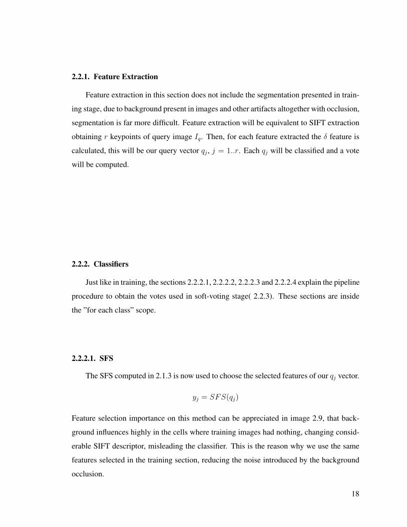
2.2.1. Feature Extraction

Feature extraction in this section does not include the segmentation presented in train-

ing stage, due to background present in images and other artifacts altogether with occlusion,

segmentation is far more difficult. Feature extraction will be equivalent to SIFT extraction

obtaining r keypoints of query image Iq. Then, for each feature extracted the δ feature is

calculated, this will be our query vector qj , j = 1..r. Each qj will be classified and a vote

will be computed.

2.2.2. Classifiers

Just like in training, the sections 2.2.2.1, 2.2.2.2, 2.2.2.3 and 2.2.2.4 explain the pipeline

procedure to obtain the votes used in soft-voting stage( 2.2.3). These sections are inside

the ”for each class” scope.

2.2.2.1. SFS

The SFS computed in 2.1.3 is now used to choose the selected features of our qj vector.

yj = SFS(qj)

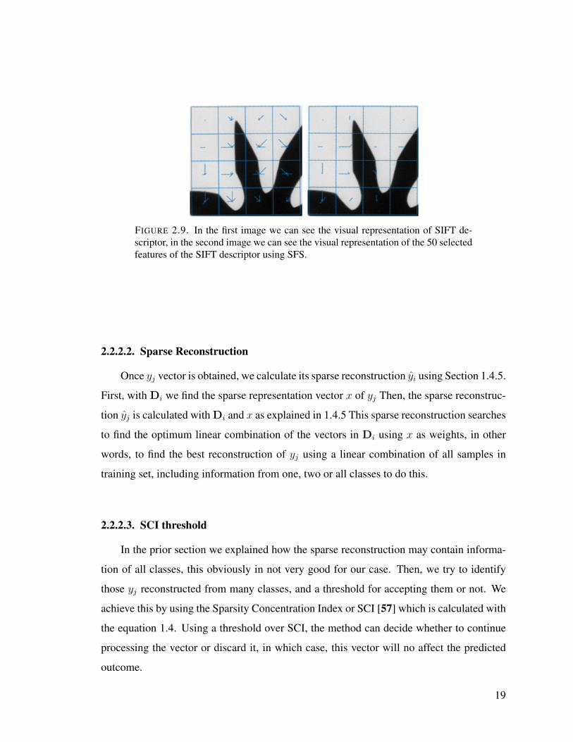
Feature selection importance on this method can be appreciated in image 2.9, that back-

ground influences highly in the cells where training images had nothing, changing consid-

erable SIFT descriptor, misleading the classifier. This is the reason why we use the same

features selected in the training section, reducing the noise introduced by the background

occlusion.

18

FIGURE 2.9. In the first image we can see the visual representation of SIFT de-scriptor, in the second image we can see the visual representation of the 50 selectedfeatures of the SIFT descriptor using SFS.

2.2.2.2. Sparse Reconstruction

Once yj vector is obtained, we calculate its sparse reconstruction yi using Section 1.4.5.

First, with Di we find the sparse representation vector x of yj Then, the sparse reconstruc-

tion yj is calculated with Di and x as explained in 1.4.5 This sparse reconstruction searches

to find the optimum linear combination of the vectors in Di using x as weights, in other

words, to find the best reconstruction of yj using a linear combination of all samples in

training set, including information from one, two or all classes to do this.

2.2.2.3. SCI threshold

In the prior section we explained how the sparse reconstruction may contain informa-

tion of all classes, this obviously in not very good for our case. Then, we try to identify

those yj reconstructed from many classes, and a threshold for accepting them or not. We

achieve this by using the Sparsity Concentration Index or SCI [57] which is calculated with

the equation 1.4. Using a threshold over SCI, the method can decide whether to continue

processing the vector or discard it, in which case, this vector will no affect the predicted

outcome.

19

FIGURE 2.10. Visual example of a few keypoints discarded by SCI threshold

2.2.2.4. KNN Classifier and Distance threshold

Usually sparse reconstruction method use as classifier a SVM [7] or reconstruction

error. Having tried these, we aim for a simpler classifier, a k - nearest neighbors is used

to classify the reconstructed vector yj retrieving not the binary prediction class or no class,

but a soft-voting normalized. Using the closest distance to a neighbor (k is not necessarily

1), we use a distanceThreshold for each class to determine if the sample is close enough

to his neighbor or too far to take a clear decision, and as consequence, discarding this from

votes.

Algorithm 1 KNN Classifier and Distances Thresholdsfor all class i 6= other do

(knnPredictedClass, knnDistance) = KNNi(yj)if knnDistance ≥ distanceThresholdknnPredictedClass then

yj ← discardedelse

distances(yj, knnPredictedClass)← knnDistance

20

It is good to remember that each KNN classifier will give us if yj belongs to the clas-

sifier class or to the class other, as every classifier was trained for a different class. With

this, each yj will give us one prediction class and one distance for each class i.

2.2.3. SoftVoting

Once all distances of every yj had been collected, the votes corresponding to each class

are added and special cases are handled; if there is no votes, it means that there where no

keypoints selected or all where discarted, then, the image belongs instantly to the other

class.

We use a soft voting approach in an attempt to trust more in those keypoints that are

closer to the original image keypoints and not only in the presence of them, improving

the classifiers performance. In order to do this, each knnDistance is considered to be

the vote. In order to use a maximization approach, all votes are calculated by substracting

knnDistance to the corresponding distanceThreshold. In the case of the other class,

there is no classifier so there is no threshold either. Finally, the predicted class will be

selected as the one with the higher votes.

Algorithm 2 Soft-voting Calculationfor all j do

for all class i 6= other dovj =

∑j distanceThresholdi − distances(yj, i)

pcj = ı

Then, the parameter minMaxDistance is calculated and used as a threshold to detect

untrusted set of votes, this is done by comparing this parameter with the standard deviation

of the votes sample, then the previous algorithm:

21

Algorithm 3 Soft-voting Classificationfor all j do

for all class i 6= other dovotes(i) =

∑pcj=i vj

if std(votes) < minMaxDistance thenpredictedClass(Iq)← 4

elsepredictedClass(Iq)← max(votes)

22

3. EXPERIMENTS AND RESULTS

This chapter contains the practical procedures used regardless our method, for this,

first the database will be introduced, then the experiments will be explained as well as

the parameters adjustment, and finally results will be presented, confusion matrices and

performances curves.

3.1. DataBase

We use a subset of GDXray database [37] created for this kind of experiments (fold-

ers B0049 though B0082). This has two main sets, training images and testing images,

although testing images will be split into validation and testing. These sets are X ray im-

ages taken from four different classes, guns, shurikens, razor and others, the other or

non − object class contains images as wide as possible, for example, castings, weldings,

fishbones, springs, bags portions that don’t include object of the 3 prior classes. Due the le-

gal difficulty to obtain a gun, we used the same gun in different rotations and environments.

The specific technicalities are explained in each subsection.

3.1.1. Training Images

There are 900 X-Ray images for training; 300 for the object classes, this is, 100 for

guns, 100 for shurikens, and 100 for razors; and 600 for the other class.

The 300 object class contained only one instance of object of the class, centered and

complete; this object has no occlusion, nor present other artifacts in the image. Images

where taken in different angles with rotations of 20◦ in X axis and rotations in Y axis

generating all possible views to be detected by SIFT keypoints.

23

FIGURE 3.1. Example images of training set (From left to right, guns, shurikens,razors and class other)

FIGURE 3.2. A gun rotating as an example of rotation of the objects

3.1.2. Testing Images

There are 1050 X ray images in testing set; 150 correspond to the object classes, this

is, 150 for guns, 150 for shurikens, and 150 for razors; and 600 correspond to the class

other.

Images are cropped arround the object (as for sliding windows approach). The 450

images with guns, razors and shurikens, contain only one object, centered and complete;

these images correspond to a object inside a bag, therefore contains other artifacts present,

background, creating occlusion of different degrees as shown in figure 3.1. The 600 images

without object are X ray images from a variety of environment, among them, the sabe bag

used in the object class, wood, fruit, weldings, other bags without object class present, etc.

Testing images are randomly divided into two sets, testing set and validation set. Testing

set is to be used for finding parameters, testing a variety of methods, try and error, etc.

Validation set was used just one time once the method and it’s parameters where defined in

order to prove the method performance.

24

FIGURE 3.3. Example of testing images, left image is the complete bag X-Ray,the right image is the cropped and oriented object.

FIGURE 3.4. Example images of testing set (From left to right, guns, shurikens,razors and class other)

25

TABLE 3.1. Distribution of images among all sets

Class Training Validation Testing

Gun 200 50 100

Shuriken 100 50 100

Razor 100 50 100

Other 500 200 400

3.2. Experiments

The experiments used to mesure performance for this method are explained on this

section. First, for testing stage, complete training set is used as explained in section 2.2.

Then, for testing and validation stage testing images are selected by a random vector which

is saved for future methods performance comparison, this selection is made by 1/3 for

validation and 2/3 for testing.

Training and validation stage is where the heavy lifting is made, trying different meth-

ods, variations of these methods, and combinations of them forged our currently method.

Validation is the repetitive stage where parameters are tuned. Then the method is trained

with these selected parameters. In subsection 3.2.1 parameters and it’s optimization is ex-

plained.

Then when method is defined and all parameters are selected, we ignore training and

validation images and use testing images (unseen for the algorithm so far). In this stage,

both, method and parameters remain untouched in such a way that every time we run it the

output values are exactly the same.

3.2.1. Parameters adjustment

There are several parameters to adjust in this method, in this section we mention the

most relevant parameters to our consideration and how they where selected for this partic-

ular set of images. We will divide them into two main method groups, by observation and

by exploration

26

3.2.1.1. Observation parameter selection

SFS contain two parameters, one is an arbitrary chosen k for the inner knn, the other is

ns the number of selected features in SFS. This parameter is selected by running SFS until

Jmax value becomes stable (Jmax stop increasing or increase is not significant), this is done

by visual inspection in the graphic Jmax vs ns as shown in picture 3.5. k is selected as the

same k in 3.2.1.2, then, selected value of s is:

s = 50

We use the same s for each classifier in order to maintain vectors of same size and a

fair comparison among the results.

FIGURE 3.5. In the top, Jmax vs number of features using SFS for each class. Inthe bottom, a zoom in to the appreciate the stabilization point of Jmax (near 50 inevery case)

27

SIFT contains several parameters, all parameters are use as default except for the

threshold for peak selection PeakThresh, which basically is a sensitivity threshold se-

lecting more or less keypoints. We use PeakThresh = 1 to avoid selecting keypoints that

are actually noise in the image as shown in figure 3.6.

FIGURE 3.6. The first image shows the original image, the second correspond tothe segmented image and third image is the mask mentioned in 2.1.1 and the fourthimage shows all SIFT keypoints filtered using the mask of third image.

3.2.1.2. Exploration parameter selection

There are several parameters founded using search by exploration among two values.

The k of K-means classifier was selected iterating with k ∈ [1, 10]. In sparse reconstruc-

tion we use default parameters, except The SCIThreshold parameter was iterated using

SCIThreshold ∈ [0, 1] using 1 decimal precision. All distance threshold where iterated

in the interval [10000, 100000] with jumps of 10000 in a for loop, parameters for each class

where selected at the same time, is meaningful to mention that the value for the other class

is 0, meaning that none yj classified as other is affected. The minMaxDistance parame-

ter is also iterated using minMaxDistance ∈ [0, 100000] using intervals of 100. Finally,

selected parameters of this section are:

k = 5

sciThreshold = 0.91

distanceTresholdP istol = 50000

distanceTresholdShuriken = 800001all SCI threshold turn out to be the same result

28

distanceTresholdRazor = 90000

minMaxDistance = 21700

In figures 3.7, 3.8, 3.9 and 3.10 we can see the accuracy for our method while we

variate one of the prior parameters while maintaining the others static.

FIGURE 3.7. We can see the accuracy behavior when variating the DistanceTresh-oldPistol, this accuracy correspond to the final performance of our method, includ-ing the four classes. We can see clearly a global optimal value at 5000.

29

FIGURE 3.8. We can see the accuracy behavior when variating the DistanceTresh-oldRazor, this accuracy correspond to the final performance of our method, includ-ing the four classes. We can see clearly a global optimal value at 9000 and then itstarts to decay. Having a higher value in this threshold compared with Pistol thresh-old shows us that the Razor class has less intraclass variance and thus the thresholdcan be more refined (lets remember that soft-voting works in a inverse normalizedapproach).

FIGURE 3.9. We can see the accuracy behavior when variating the DistanceTresh-oldShuriken, this accuracy correspond to the final performance of our method, in-cluding the four classes. We can see clearly a global optimal value at 8000 andthen it starts to decay. As with DistanceThresholdRazor, the shuriken class has lessvariance within, and its threshold can be more refined.

30

FIGURE 3.10. We can see the accuracy behavior when variating the minMaxDis-tance, this accuracy correspond to the final performance of our method, includingthe four classes. We can see many local optimal values, however, there is a globaloptimal value at 21700 and then it starts to decay

3.3. Curves

As we have three classifiers (guns, shurikens and razors), for each parameter, we

present the Precision-Recall curves for each one, and using the mean of these curves, we

calculate an Precision-Recall curve for the general multi-class classification.

SCI: For each class we present the precision recall curves while variating the SCI

threshold. We can appreciate that curves behavior variates for the different classes, this

shows that SCI acts within classes, and not isolated one from another.

31

FIGURE 3.11. Precision-Recall Curves variating SCI parameter

Distances thresholds: For each class, we present the Precision-Recall curves vari-

ating three different parameters distanceTresholdP istol, distanceTresholdShuriken

and distanceTresholdRazor. We can see that there is no optimal general solution, this

because the intraclass variance, a pistol have more variability among his keypoints than

shuriken class. As we variate a particular distance threshold, the other classes performance

variates, we deduce that this is because these are not completely disjoint classes, otherwise,

a simple knn with k=1 would be sufficient to solve this problem.

32

FIGURE 3.12. Precision-Recall Curves variating distanceTresholdP istol parameter

FIGURE 3.13. Precision-Recall Curves variating distanceTresholdShuriken parameter

33

FIGURE 3.14. Precision-Recall Curves variating distanceTresholdRazor parameter

minMaxDistance: For each class we present the Precision-Recall curves while vari-

ating the minMaxDistance parameter, we can see that different than SCI threshold, the

minMaxDistance behavior is similar in all classes, this is because it is a parameter that

affect within the class.

34

FIGURE 3.15. Precision-Recall Curves variating minMaxDistance parameter

3.4. Results

Two different experiments were made

A) 3 binary classifiers: Pistol vs. No Pistol, Shuriken vs. No shuriken, Razor vs. No

razor

B) 4-class classifier: Pistol, Shuriken, Razor and Others. This classifier is constructed

with the three classifiers above, when none of them classifies as their class, the images is

classified as other, when one of them classifies as their class that is the predicted class, and

when more then one classifies as their class, we use the soft-voting values to decide.

The numeric results for these two experiments in validation and testing stage are shown

ahead.

3.4.1. Validation Performance

Here we present the accuracy, precision and recall obtained in Validation set after

parameter tuning (our optim found).

35

TABLE 3.2. Precision & Recall for validation set in experiment (A)

Pistol Shuriken Razor

Pr Re Pr Re Pr Re

Ours 1.00 0.97 1.00 0.99 0.98 0.93

TABLE 3.3. Accuracy for each detector in validation set (in percentages) in exper-iment (B)

Pistol Shuriken Razor Other Total

Ours 97.14 99.14 91.71 90 94.5

3.4.2. Comparison of different methods

In order to have a referral for our method performance, in table 3.4 and 3.5 we compare

our method.

In the first section, we evaluate the two most popular Convolutional Neural Network

(CNN) models related with ImageNet: the AlexNet model proposed by Krizhevsky [20]

and the GoogleNet model proposed by Szegedy [52]. Also we include Adaptive Implicit

Shape Model (AISM), wich was presented originally in [47] for object recognition in bag-

gage screening.

In the second section, we compare it with basic general methods. For each method,

we use a similar approach as for our method, we extract SIFT from training images and

use them to train the models, then in testing we classify each SIFT extracted from the

query image using the corresponding method (Knn, SVM, AdaBoost or SRC) and use its

predicted class as vote, then the predicted class of the image is calculated by counting votes

in each classifier.

36

TABLE 3.4. Precision & Recall for each detector in experiment (A)

Pistol Shuriken Razor

Pr Re Pr Re Pr Re

Sparse-Knn(Ours) 0.99 0.97 1.00 0.99 0.97 0.94

GoogleNet [20] 0.83 1.00 0.99 1.00 0.84 0.95

AISM [47] 0.97 0.97 0.95 0.96 0.99 0.99

AlexNet [52] 0.85 0.99 1.00 1.00 0.90 0.72

Knn 0.92 1.00 1.00 0.93 0.99 0.88

SVM 0.90 0.99 1.00 0.85 0.51 1.00

AdaBoost [44] 1.00 0.87 1.00 0.86 0.98 0.87

SRC 0.75 1.00 0.80 1.00 0.45 0.98

TABLE 3.5. Accuracy for each detector (in percentages) in experiment (B)

Pistol Shuriken Razor Other Total

Sparse-Knn(Ours) 97.0 99.4 91.9 90.6 94.7

GoogleNet [20] 100.0 100.0 95.0 90.0 96.3

AISM [47] 96.0 94.0 99.0 92.5 95.4

AlexNet [52] 99.0 100.0 72.0 93.5 91.2

Knn 93 93 87 83 89

SVM 91 86 86 79 85.5

AdaBoost [44] 87 86 84 60 79.25

SRC 79 83 52 80 73.5

On these comparisons we can see the power of our method, with a higher accuracy than

all classic methods presented and competing with others powerful methods state of the art

like AISM and deep learning methods, noting that the best performance was achieved by

GoogleNet with a 96.3% accuracy. In the table 3.4 we can see that the weakness of our

37

methods is the class razor blades, with a 0.94 recall vs. a 0.97 and a 0.99 in pistol and

shurikens respectively. It is our believe that this is produced by the thinness of the object.

FIGURE 3.16. Confusion Matrix for Sparse-Knn in testing set

38

4. CONCLUSION

The validation set and testing set gave similar results, proving that data is stable. Both

datasets where obtained from the same parent set, these being chosen in a random manner,

with this, if both results where different, it would mean that data was not equivalent in both.

This ensures that results are not highly related with the selection of these sets.

Feature selection method SFS has proven to be efficient with SIFT features, reducing

the dimensionality from 128 to 50, we do not say that s = 50 is a mandatory number, but

rather a parameter to be tuned to fit the need of every problem. This selection let us deal

with the background noise of the images thanks that the training set has clear images of the

objects.

Conceptually, soft voting is a better approach than binary voting system. In our method

this has been proven right. We have tried several types of votes, such as max distance of

knn, average distance of knn, SCI, error reconstruction over sparse reconstruction, etc.

being the best the inverse of the distance as explained in 2.2.3. This leads us to conclude

that if representative vote system can be found, soft voting is the most accurate approach

to follow.

Even thought our method shows great performance, deep learning based method have

similar results and even better in some cases, GoogleNet reaches a 96.3% accuracy, while

AlexNet gets a 90.7% (a 4.7% lower than ours). This behavior can be attributed to the

fact that GoogleNet was thought to address the object detection problem while AlexNet, as

simpler model, that was thought just for classification. Hence, GoogleNet could be more

robust to noisy backgrounds which is the main problem of this work

Sparse techniques are very useful in different environments. For example, using the

error reconstruction [57] can be very useful for iris recognition, a more complex model

based on SRC [33] can be very powerful when it comes to face recognition. In our case,

these methods won’t give that good results, but if used as a hidden variable, can provide

a helpful index, SCI let us separate those query vector that are reconstructed using many

classes and therefore don’t belong to any of those, detecting false positive detection and

39

correcting them on due time. Hence forth, while distance thresholds are useful within the

binary class, SCI thresholds are needed when we deal with several classes, especially with

those close to each other (p.e. knife sharp and shuriken sharp).

Dealing with rigid objects, knn has proven to be more efficient than SVM in time and

accuracy, and using parametric thresholds it boosts up the accuracy results in our method.

This reminds us of the principle of Occam’s Razor; the simpler solution is most commonly

the best solution.

Unfortunately our method is not easily extendable to other classes. If we refer to

coding, our method is pretty simple. Just add the names, paths and number of classes i. But

then, SFS would have to be calculated again; the distance thresholds and other parameters.

This is true because the new class might be very similar to a prior class and thresholds

should be more refined, or the class will be very distant to know classes and threshold

could remain without variation. Also, we would have to make sure that the class other

doesn’t contain images of the new class. With this, our method is not easily extendable.

Our method considers one view. Then, as future work an extension of it could consider

multiple views like [36]. This is likely possible as we use SIFT as a descriptor. Lowe said

that key points can be successfully detected in views with 20 degrees rotation. Keypoints

are effective for matching them to an object. Multiple views can provide sturdiness to our

model, and its filters can be applied in order to recognize those keypoints of interest as done

in [31, 35].

40

References

[1] M. Aharon, M. Elad, and A. Bruckstein. k -svd: An algorithm for designing over-

complete dictionaries for sparse representation. Signal Processing, IEEE Transac-

tions on, 54(11):4311–4322, Nov 2006.

[2] Paul T. Bartone, Bjorn Heige Jonsen, Jarle Eid, John M. Violangi, and Jon Chris-

tian Laberg. Enhancing Human Performance in Security Operations. Charles C

Thomas, 2010.

[3] Herbert Bay, Tinne Tuytelaars, and Luc Van Gool. Surf: Speeded up robust fea-

tures. In Computer vision–ECCV 2006, pages 404–417. Springer, 2006.

[4] Serge Belongie, Jitendra Malik, and Jan Puzicha. Shape matching and object

recognition using shape contexts. Pattern Analysis and Machine Intelligence,

IEEE Transactions on, 24(4):509–522, 2002.

[5] Garrick Blalock, Vrinda Kadiyali, and Daniel H Simon. The Impact of Post-9/11

Airport Security Measures on the Demand for Air Travel. The Journal of Law and

Economics, 50(4):731–755, November 2007.

[6] Anton Bolfing, Tobias Halbherr, and Adrian Schwaninger. How image based fac-

tors and human factors contribute to threat detection performance in X-ray aviation

security screening. In Andreas Holzinger, editor, HCI and Usability for Education

and Work, volume 5298 of Lecture Notes in Computer Science, pages 419–438.

Springer Berlin Heidelberg, 2008.

[7] Corinna Cortes and Vladimir Vapnik. Support-vector networks. Mach. Learn.,

20(3):273–297, September 1995.

[8] Romeu Ricardo da Silva and Domingo Mery. State-of-the-art of weld seam in-

spection by radiographic testing: part i–image processing. Materials Evaluation,

65(6):643–647, 2007.

41

[9] Navneet Dalal and Bill Triggs. Histograms of oriented gradients for human detec-

tion. In Proceedings of the 2005 IEEE Computer Society Conference on Computer

Vision and Pattern Recognition (CVPR’05) - Volume 1 - Volume 01, CVPR ’05,

pages 886–893, Washington, DC, USA, 2005. IEEE Computer Society.

[10] Ankit Dixit. Adaptive kmeans clustering for color and gray image.

(http://www.mathworks.com/matlabcentral/fileexchange/45057-adaptive-kmeans-

clustering-for-color-and-gray-image). Matlab Central, File Exchange, January

2014.

[11] Bradley Efron, Trevor Hastie, Iain Johnstone, Robert Tibshirani, et al. Least angle

regression. The Annals of statistics, 32(2):407–499, 2004.

[12] Pedro F. Felzenszwalb, Ross B. Girshick, David McAllester, and Deva Ramanan.

Object detection with discriminatively trained part-based models. IEEE Trans.

Pattern Anal. Mach. Intell., 32(9):1627–1645, September 2010.

[13] Greg Flitton, Toby P Breckon, and Najla Megherbi. A comparison of 3D interest

point descriptors with application to airport baggage object detection in complex

CT imagery. Pattern Recognition, 46(9):2420–2436, September 2013.

[14] Greg Flitton, Andre Mouton, and Toby P Breckon. Object classification in 3D

baggage security computed tomography imagery using visual codebooks. Pattern

Recognition, 48(8):2489–2499, August 2015.

[15] T Franzel, U Schmidt, and S Roth. Object Detection in Multi-view X-Ray Images.

Pattern Recognition, 2012.

[16] Harold Hotelling. Analysis of a complex of statistical variables into principal com-

ponents. Journal of educational psychology, 24(6):417, 1933.

[17] M. A. Wong J. A. Hartigan. Algorithm as 136: A k-means clustering algorithm.

Journal of the Royal Statistical Society. Series C (Applied Statistics), 28(1):100–

108, 1979.

42

[18] Anil K Jain and Hong Chen. Matching of dental x-ray images for human identifi-

cation. Pattern recognition, 37(7):1519–1532, 2004.

[19] Pamela M Keagy, Bahram Parvin, and Thomas F Schatzki. Machine recognition of

navel orange worm damage in x-ray images of pistachio nuts. LWT-Food Science

and Technology, 29(1):140–145, 1996.

[20] Alex Krizhevsky, Ilya Sutskever, and Geoffrey E. Hinton. Imagenet classification

with deep convolutional neural networks. In F. Pereira, C.J.C. Burges, L. Bottou,

and K.Q. Weinberger, editors, Advances in Neural Information Processing Systems

25, pages 1097–1105. Curran Associates, Inc., 2012.

[21] Daniel T Larose. k-nearest neighbor algorithm. Discovering Knowledge in Data:

An Introduction to Data Mining, pages 90–106, 2005.

[22] David G. Lowe. Object recognition from local scale-invariant features. In Pro-

ceedings of the International Conference on Computer Vision-Volume 2 - Volume

2, ICCV ’99, pages 1150–, Washington, DC, USA, 1999. IEEE Computer Society.

[23] David G. Lowe. Distinctive image features from scale-invariant keypoints. Int. J.

Comput. Vision, 60(2):91–110, November 2004.

[24] Jiebo Luo and D. Crandall. Color object detection using spatial-color joint proba-

bility functions. Trans. Img. Proc., 15(6):1443–1453, June 2006.

[25] Julien Mairal, Francis Bach, Jean Ponce, and Guillermo Sapiro. Online dictionary

learning for sparse coding. In Proceedings of the 26th Annual International Con-

ference on Machine Learning, ICML ’09, pages 689–696, New York, NY, USA,

2009. ACM.

[26] Julien Mairal, Francis Bach, Jean Ponce, and Guillermo Sapiro. Online learning

for matrix factorization and sparse coding. J. Mach. Learn. Res., 11:19–60, March

2010.

[27] S.G. Mallat and Zhifeng Zhang. Matching pursuits with time-frequency dictionar-

ies. Trans. Sig. Proc., 41(12):3397–3415, December 1993.

43

[28] N Megherbi, Jiwan Han, T P Breckon, and G T Flitton. A comparison of classifica-

tion approaches for threat detection in CT based baggage screening. In Image Pro-

cessing (ICIP), 2012 19th IEEE International Conference on, pages 3109–3112.

IEEE, 2012.

[29] D Mery. Computer Vision for X-Ray Testing. Springer, 2015.

[30] D Mery. Inspection of Complex Objects Using Multiple-X-Ray Views.

IEEE/ASME Transactions on Mechatronics, 20(1):338–347, 2015.

[31] D. Mery, V. Riffo, I. Zuccar, and C. Pieringer. Automated x-ray object recognition

using an efficient search algorithm in multiple views. In Proceedings of 9th IEEE

CVPR workshop on Perception Beyond the Visible Spectrum (PBVS’2013), Jun.

24th, Portland, USA, pages 1–7, 2013.

[32] Domingo Mery. BALU: A Matlab toolbox for computer vision, pattern recognition

and image processing (http://dmery.ing.puc.cl/ index.php/balu), 2011.

[33] Domingo Mery and Kevin Bowyer. Automatic facial attribute analysis via adaptive

sparse representation of random patches. Pattern Recogn. Lett., 68(P2):260–269,

December 2015.

[34] Domingo Mery, German Mondragon, Vladimir Riffo, and Irene Zuccar. Detection

of regular objects in baggage using multiple x-ray views. Insight-Non-Destructive

Testing and Condition Monitoring, 55(1):16–20, 2013.

[35] Domingo Mery and V. Riffo. Automated object recognition in baggage screening

using multiple x-ray views. In 52nd Annual Conference of the British Institute for

Non-Destructive Testing. Telford, UK, Sep. 10-12, 2013.

[36] Domingo Mery and Vladimir Riffo. Automated object recognition using multiple

x-ray views. MATERIALS EVALUATION, 72(11):1362–1372, 2014.

[37] Domingo Mery, Vladimir Riffo, Uwe Zscherpel, German Mondragon, Ivan Lillo,

Irene Zuccar, Hans Lobel, and Miguel Carrasco. GDXray: The database of X-ray

44

images for nondestructive testing. Journal of Nondestructive Evaluation, 34(4):1–

12, 2015.

[38] S. Michel, S.M. Koller, J.C. de Ruiter, R. Moerland, M. Hogervorst, and

A. Schwaninger. Computer-based training increases efficiency in X-ray image in-

terpretation by aviation security screeners. In Security Technology, 2007 41st An-

nual IEEE International Carnahan Conference on, pages 201–206, Oct 2007.

[39] A Mouton, G T Flitton, and S Bizot. An evaluation of image denoising techniques

applied to CT baggage screening imagery. In IEEE International Conference on

Industrial Technology (ICIT 2013). IEEE, 2013.

[40] Andre Mouton and Toby P Breckon. Materials-based 3D segmentation of un-

known objects from dual-energy computed tomography imagery in baggage se-

curity screening. Pattern Recognition, 48(6):1961–1978, June 2015.

[41] European Parliament. Aviation security with a special focus on security scanners.

European Parliament Resolution (2010/2154(INI)), pages 1–10, October 2012.

[42] K. Pearson. On lines and planes of closest fit to systems of points in space. Philo-

sophical Magazine, 2(6):559–572, 1901.

[43] Jaishanker K. Pillai, Vishal M. Patel, Rama Chellappa, and Nalini K. Ratha. Secure

and robust iris recognition using random projections and sparse representations.

IEEE Trans. Pattern Anal. Mach. Intell., 33(9):1877–1893, September 2011.

[44] R. Polikar. Ensemble based systems in decision making. Circuits and Systems

Magazine, IEEE, 6(3):21–45, Third 2006.

[45] V Riffo and D Mery. Active X-ray testing of complex objects. Insight-Non-

Destructive Testing and Condition Monitoring, 54(1):28–35, 2012.

[46] V Riffo and D Mery. Automated detection of threat objects using Adapted Implicit

Shape Model. IEEE Transactions on Systems, Man, and Cybernetics: Systems,

2015. (In Press).

45

[47] Vladimir Riffo and Domingo Mery. Automated detection of threat objects using

adapted implicit shape model. 2015.

[48] Thomas Ruckstieß, Christian Osendorfer, and Patrick Smagt. AI 2011: Advances

in Artificial Intelligence: 24th Australasian Joint Conference, Perth, Australia, De-

cember 5-8, 2011. Proceedings, chapter Sequential Feature Selection for Classifi-

cation, pages 132–141. Springer Berlin Heidelberg, Berlin, Heidelberg, 2011.

[49] Thomas Ruckstieß, Christian Osendorfer, and Patrick van der Smagt. Sequential

feature selection for classification. In Dianhui Wang and Mark Reynolds, editors,

AI 2011: Advances in Artificial Intelligence, volume 7106 of Lecture Notes in Com-

puter Science, pages 132–141. Springer Berlin Heidelberg, 2011.

[50] Adrian Schwaninger, Anton Bolfing, Tobias Halbherr, Shaun Helman, Andrew

Belyavin, and Lawrence Hay. The impact of image based factors and training

on threat detection performance in X-ray screening. In Proceedings of the 3rd

International Conference on Research in Air Transportation, ICRAT 2008, pages

317–324, 2008.

[51] Thomas J Smith, Robert A Henning, Michael G Wade, and Thomas Fisher. Vari-

ability in human performance. CRC Press, 2014.

[52] Christian Szegedy, Wei Liu, Yangqing Jia, Pierre Sermanet, Scott Reed, Dragomir

Anguelov, Dumitru Erhan, Vincent Vanhoucke, and Andrew Rabinovich. Going

deeper with convolutions. In CVPR 2015, 2015.

[53] Hotaka Takizawa, Shinji Yamamoto, Tohru Matsumoto, Yukio Tateno, Takeshi

Iinuma, and Mitsuomi Matsumoto. Recognition of lung nodules from x-ray ct

images using 3d markov random field models. In Medical Imaging 2002, pages

716–725. International Society for Optics and Photonics, 2002.

[54] I. Tosic and P. Frossard. Dictionary learning. Signal Processing Magazine, IEEE,

28(2):27–38, 2011.

46

[55] D Turcsany, A Mouton, and T P Breckon. Improving feature-based object recog-

nition for X-ray baggage security screening using primed visualwords. In IEEE

International Conference on Industrial Technology (ICIT 2013), pages 1140–1145.

[56] I Uroukov and R Speller. A preliminary approach to intelligent x-ray imaging for

baggage inspection at airports. Signal Processing Research, 2015.

[57] John Wright, Allen Y. Yang, Arvind Ganesh, S. Shankar Sastry, and Yi Ma. Robust

face recognition via sparse representation. IEEE Trans. Pattern Anal. Mach. Intell.,

31(2):210–227, February 2009.

[58] G. Zentai. X-ray imaging for homeland security. IEEE International Workshop

on Imaging Systems and Techniques (IST 2008), pages 1–6, Sept. 2008.

[59] N Zhang and J Zhu. A study of X-ray machine image local semantic features

extraction model based on bag-of-words for airport security. International Journal

on Smart Sensing and Intelligent Systems, 8(1):45–64, 2015.

[60] Xiao-Guang Zhang, Jian-Jian Xu, and Guang-Ying Ge. Defects recognition on x-

ray images for weld inspection using svm. In Machine Learning and Cybernetics,

2004. Proceedings of 2004 International Conference on, volume 6, pages 3721–

3725. IEEE, 2004.

47