Sparse Matrix Code Dependence Analysis Simplification at Compile Time MAHDI SOLTAN MOHAMMADI, University of Arizona KAZEM CHESHMI, University of Toronto GANESH GOPALAKRISHNAN, University of Utah MARY HALL, University of Utah MARYAM MEHRI DEHNAVI, University of Toronto ANAND VENKAT, Intel Corporation TOMOFUMI YUKI, Univ. Rennes, Inria, CNRS, IRISA MICHELLE MILLS STROUT, University of Arizona Analyzing array-based computations to determine data dependences is useful for many applications including automatic parallelization, race detection, computation and communication overlap, verification, and shape analysis. For sparse matrix codes, array data dependence analysis is made more difficult by the use of index arrays that make it possible to store only the nonzero entries of the matrix (e.g., in A[B[i]], B is an index array). Here, dependence analysis is often stymied by such indirect array accesses due to the values of the index array not being available at compile time. Consequently, many dependences cannot be proven unsatisfiable or determined until runtime. Nonetheless, index arrays in sparse matrix codes often have properties such as monotonicity of index array elements that can be exploited to reduce the amount of runtime analysis needed. In this paper, we contribute a formulation of array data dependence analysis that includes encoding index array properties as universally quantified constraints. This makes it possible to leverage existing SMT solvers to determine whether such dependences are unsatisfiable and significantly reduces the number of dependences that require runtime analysis in a set of eight sparse matrix kernels. Another contribution is an algorithm for simplifying the remaining satisfiable data dependences by discovering equalities and/or subset relationships. These simplifications are essential to make a runtime-inspection-based approach feasible. Additional Key Words and Phrases: Dependence Analysis, Sparse Matrices, Inspector Simplification, Decision Procedure, SMT 1 INTRODUCTION Data dependence analysis answers questions about which memory accesses in which loop iterations access the same memory location thus creating a partial ordering (or dependence) between loop iterations. Determining this information enables iteration space slicing [Pugh and Rosser 1997], provides input to race detection, makes automatic parallelization and associated optimizations such as tiling or communication/computation overlap possible, and enables more precise data-flow analysis, or abstract interpretation. A data dependence exists between two array accesses that (1) access the same array element with at least one access being a write and (2) that access occurs within the loop bounds for each of the accesses’ statement(s). These conditions for a data dependence has been posed as a constraint-based decision problem [Banerjee et al. 1993], a data-flow analysis with polyhedral set information [Feautrier 1991], and linear memory access descriptors [Paek et al. 2002]. However, such approaches require a runtime component when analyzing codes with indirect Authors’ addresses: Mahdi Soltan Mohammadi, Department of Computer Science, University of Arizona, kingmahdi@cs. arizona.edu; Kazem Cheshmi, Department of Computer Science, University of Toronto, [email protected]; Ganesh Gopalakrishnan, School of Computing, University of Utah, [email protected]; Mary Hall, School of Computing, University of Utah, [email protected]; Maryam Mehri Dehnavi, Department of Computer Science, University of Toronto, mmehride@ cs.toronto.edu; Anand Venkat, Intel Corporation, [email protected]; Tomofumi Yuki, Univ. Rennes, Inria, CNRS, IRISA, [email protected]; Michelle Mills Strout, Department of Computer Science, University of Arizona, mstrout@cs. arizona.edu. , Vol. 1, No. 1, Article . Publication date: July 2018. arXiv:1807.10852v1 [cs.PL] 27 Jul 2018
Transcript
Sparse Matrix Code Dependence Analysis Simplification atCompile Time
MAHDI SOLTAN MOHAMMADI, University of Arizona
KAZEM CHESHMI, University of Toronto
GANESH GOPALAKRISHNAN, University of Utah
MARY HALL, University of Utah
MARYAM MEHRI DEHNAVI, University of Toronto
ANAND VENKAT, Intel CorporationTOMOFUMI YUKI, Univ. Rennes, Inria, CNRS, IRISAMICHELLE MILLS STROUT, University of Arizona
Analyzing array-based computations to determine data dependences is useful for many applications including
automatic parallelization, race detection, computation and communication overlap, verification, and shape
analysis. For sparse matrix codes, array data dependence analysis is made more difficult by the use of index
arrays that make it possible to store only the nonzero entries of the matrix (e.g., in A[B[i]], B is an index array).
Here, dependence analysis is often stymied by such indirect array accesses due to the values of the index
array not being available at compile time. Consequently, many dependences cannot be proven unsatisfiable
or determined until runtime. Nonetheless, index arrays in sparse matrix codes often have properties such
as monotonicity of index array elements that can be exploited to reduce the amount of runtime analysis
needed. In this paper, we contribute a formulation of array data dependence analysis that includes encoding
index array properties as universally quantified constraints. This makes it possible to leverage existing SMT
solvers to determine whether such dependences are unsatisfiable and significantly reduces the number of
dependences that require runtime analysis in a set of eight sparse matrix kernels. Another contribution is an
algorithm for simplifying the remaining satisfiable data dependences by discovering equalities and/or subset
relationships. These simplifications are essential to make a runtime-inspection-based approach feasible.
Additional Key Words and Phrases: Dependence Analysis, Sparse Matrices, Inspector Simplification, Decision
Procedure, SMT
1 INTRODUCTIONData dependence analysis answers questions about which memory accesses in which loop iterations
access the same memory location thus creating a partial ordering (or dependence) between loop
iterations. Determining this information enables iteration space slicing [Pugh and Rosser 1997],
provides input to race detection, makes automatic parallelization and associated optimizations
such as tiling or communication/computation overlap possible, and enables more precise data-flow
analysis, or abstract interpretation. A data dependence exists between two array accesses that (1)
access the same array element with at least one access being a write and (2) that access occurs within
the loop bounds for each of the accesses’ statement(s). These conditions for a data dependence
has been posed as a constraint-based decision problem [Banerjee et al. 1993], a data-flow analysis
with polyhedral set information [Feautrier 1991], and linear memory access descriptors [Paek et al.
2002]. However, such approaches require a runtime component when analyzing codes with indirect
Authors’ addresses: Mahdi Soltan Mohammadi, Department of Computer Science, University of Arizona, kingmahdi@cs.
arizona.edu; Kazem Cheshmi, Department of Computer Science, University of Toronto, [email protected]; Ganesh
Gopalakrishnan, School of Computing, University of Utah, [email protected]; Mary Hall, School of Computing, University
of Utah, [email protected]; Maryam Mehri Dehnavi, Department of Computer Science, University of Toronto, mmehride@
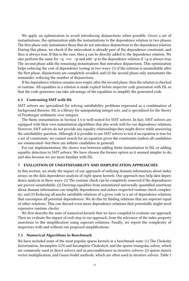
Fig. 1. Compressed Sparse Row (CSR) sparse matrix format. The val array stores the nonzeros by packingeach row in contiguous locations. The rowptr array points to the start of each row in the val array. The colarray is parallel to val and maps each nonzero to the corresponding column.
memory accesses (e.g., A[B[i]], B being an index array) such as those that occur in sparse matrix
codes. In this paper, we present an approach to improve the precision of compile-time dependence
analysis for sparse matrix codes and simplification techniques for decreasing the complexity of any
remaining runtime checks.
Sparse matrix computations occur in many codes, such as graph analysis, partial differential
equation solvers, and molecular dynamics solvers. Sparse matrices save on storage and computation
by only storing the nonzero values in a matrix. Figure 1 illustrates one example of how the sparse
matrix vector multiplication (®y = A®x ) can be written to use a common sparse matrix format called
compressed sparse row (CSR). In CSR, the nonzeros are organized by row, and for each nonzero,
the column for that nonzero is explicitly stored. Since the percentage of nonzeros in a matrix can
be less than 1%, sparse matrix formats are critical for many computations to fit into memory and
execute in a reasonable amount of time. Unfortunately, the advantage sparse matrices have on
saving storage compared to dense matrices comes with the cost of complicating program analysis.
Compile-time only approaches resort to conservative approximation [Barthou et al. 1997; Paek et al.
2002]. Some approaches use runtime dependence tests to complement compile time analysis and
obtain more precise answers [Oancea and Rauchwerger 2012; Pugh and Wonnacott 1995; Rus et al.
2003]. Runtime dependence information is also used to detect task-graph or wavefront parallelism
that arises due to the sparsity of dependences [Rauchwerger et al. 1995a; Saltz et al. 1991; Streit
et al. 2015].
The data dependence analysis approach presented here is constraint-based. Some constraint-
based data dependence analysis approaches [Pugh and Wonnacott 1994, 1995, 1998; Venkat et al.
2016] represent the index arrays in sparse matrix computations as uninterpreted functions in
the data dependence relations. For example, the loop bounds for the k loop in Figure 1 can be
represented as rowptr (i) ≤ k < rowptr (i + 1). Previous work by others generates simplified
constraints at compile time that can then be checked at runtime with the goal of finding fully
parallel loops [Pugh and Wonnacott 1995]. We build on the previous work of [Venkat et al. 2016].
In that work, dependences in a couple of sparse matrix codes were determined unsatisfiable
manually, simplified using equalities found through a partial ordering of uninterpreted function
terms, or approximated by removing enough constraints to ensure a reasonable runtime analysis
complexity. In this paper, we automate the determination of unsatisfactory data dependences, find
equalities using the Integer Set Library (ISL) [Verdoolaege 2010], have developed ways to detect
Fig. 2. This figure shows the overview of our approach to eliminate or simplify dependences from sparsecomputation utilizing domain information.
data dependence subsets for simplifying runtime analysis, and perform an evaluation with eight
popular sparse kernels.
In this paper, we have two main goals: (1) prove as many data dependences as possible to beunsatisfiable, thus reducing the number of dependences that require runtime tests; and (2) simplify thesatisfiable data dependences so that a runtime inspector for them has complexity less than or equal to theoriginal code. Figure 2 shows an overview of our approach.We use the ISL library [Verdoolaege 2018]
like an SMT solver to determine which data dependences are unsatisfiable. Next, we manipulate
any remaining dependence relations using IEGenLib [Strout et al. 2016] and ISL libraries to discover
equalities that lead to simplification.
Fortunately, much is known about the index arrays that represent sparse matrices as well as the
assumptions made by the numerical algorithms that operate on those matrices. For example, in the
CSR representation shown in Figure 1, the rowptr index array is monotonically strictly increasing.
In Section 3.1 we explain how such information can be used to add more inequality and equality
constraints to a dependence relation. The new added constraints in some cases cause conflicts, and
hence we can detect that those relations are unsatisfiable.
The dependences that cannot be shown as unsatisfiable at compile time, still require runtime
tests. For those dependences, the goal is to simplify the constraints and reduce the overhead of any
runtime test. Sometimes index array properties can be useful for reducing the complexity of runtime
inspector by finding equalities that are implied by the dependence constraints in combination with
assertions about the index arrays. The equalities such as i = col(m′) can help us remove a loop
level from the inspector, i in the example. Since some equality constraint would allow us deduce
value of an iterator in the inspector from another one, e.g, we can deduce i values fromm′values
using i = col(m′). Another simplification involves determining when data dependence relations for
a code are involved in a subset relationship. When this occurs, runtime analysis need only occur
for the superset.
This paper makes the following contributions:
(1) An automated approach for the determination of unsatisfiable dependences in sparse codes.
(2) An implementation of an instantiation-based decision procedure that discovers equality
relationships in satisfiable dependences.
(3) An approach that discovers subset relationships in satisfiable dependences thus reducing
run-time analysis complexity further.
(4) A description of common properties of index arrays arising in sparse matrix computations,
expressed as universally quantified constraints.
(5) Evaluation of the utility of these properties for determining unsatisfiability or simplifying
dependences from a suite of real-world sparse matrix codes.
where ®I and ®I ′ are iteration vector instances from the same loop nest, F and G are array index
expressions to the same array with at least one of the accesses being a write, and Bounds(®I ) expandsto the loop nest bounds for the ®I iteration vectors. In this paper, the term dependence relation is
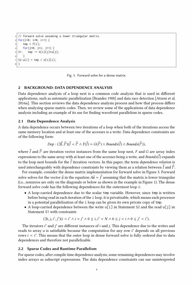
used interchangeably with dependence constraints by viewing them as a relation between ®I and ®I ′.For example, consider the dense matrix implementation for forward solve in Figure 3. Forward
solve solves for the vector ®u in the equation A®u = ®f assuming that the matrix is lower triangular
(i.e., nonzeros are only on the diagonals or below as shown in the example in Figure 1). The dense
forward solve code has the following dependences for the outermost loop i:
• A loop-carried dependence due to the scalar tmp variable. However, since tmp is written
before being read in each iteration of the i loop, it is privatizable, which means each processor
in a potential parallelization of the i loop can be given its own private copy of tmp.• A loop-carried dependence between the write u[i] in Statement S2 and the read u[j] in
Statement S1 with constraints
(∃i, j, i ′, j ′)(i < i ′ ∧ i = j ′ ∧ 0 ≤ i, i ′ < N ∧ 0 ≤ j < i ∧ 0 ≤ j ′ < i ′).
The iterators i ′ and j ′ are different instances of i and j. This dependence due to the writes and
reads to array u is satisfiable because the computation for any row i ′ depends on all previous
rows i < i ′. This means that the outer loop in dense forward solve is fully ordered due to data
dependences and therefore not parallelizable.
2.2 Sparse Codes and Runtime ParallelismFor sparse codes, after compile time dependence analysis, some remaining dependences may involve
index arrays as subscript expressions. The data dependence constraints can use uninterpreted
Fig. 4. Forward solve for a sparse matrix in compressed sparse row (CSR).
functions to represent the index arrays at compile time. Because the values of the index arrays
are unknown until run time, proving such dependences are unsatisfiable may require runtime
dependence testing. However, even when dependences arise at runtime, it still may be possible
to implement a sparse parallelization called wavefront parallelization. Identifying wavefront par-
allelizable loops combines compile time and runtime analyses. The compiler generates inspector
code to find the data dependence graph at runtime.
We now consider the sparse forward solve with Compressed Sparse Row CSR format in Figure 4.
We are interested in detecting loop-carried dependences of the outermost loop. There are two pairs
of accesses on array u in S1 and S2 that can potentially cause loop-carried dependences: u[col[k]](read), u[i] (write); and u[i] (write), u[i] (write). The constraints for the two dependence tests
are shown in the following.
Dependences for the write/write u[i] in S2:
(1) i = i ′ ∧ i < i ′ ∧ 0 ≤ i < N ∧ 0 ≤ i ′ < N
∧rowptr (i) ≤ k < rowptr (i + 1) ∧ rowptr (i ′) ≤ k ′ < rowptr (k ′ + 1)
(2) i = i ′ ∧ i ′ < i ∧ 0 ≤ i < N ∧ 0 ≤ i ′ < N
∧rowptr (i) ≤ k < rowptr (i + 1) ∧ rowptr (i ′) ≤ k ′ < rowptr (k ′ + 1)
Dependences for read u[col[k]] and write u[i] in S1, and S2:
(3) i = col(k ′) ∧ i < i ′ ∧ 0 ≤ i < N ∧ 0 ≤ i ′ < N ∧rowptr (i ′) ≤ k ′ < rowptr (i ′ + 1)
(4) i = col(k ′) ∧ i ′ < i ∧ 0 ≤ i < N ∧ 0 ≤ i ′ < N ∧rowptr (i ′) ≤ k ′ < rowptr (i ′ + 1)
These dependences can be tested at runtime when concrete interpretations for the index arrays
(contents of arrays rowptr and col) are available. The runtime dependence analyzers, called
inspectors [Saltz et al. 1991], may be generated from the dependence constraints [Venkat et al. 2016].
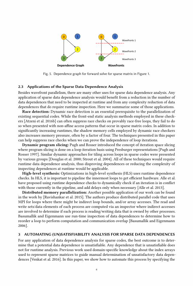
Suppose the matrix in the forward solve code in Figure 4 had the nonzero pattern as in Fig-
ure 1. The runtime check would create the dependence graph for this example based on the four
dependences above as shown in Figure 5. Once the dependence graph is constructed a breadth-first
traversal of the dependence graph can derive sets of iterations that may be safely scheduled in
parallel without a dependence violations, with each level set being called a wavefront as shown in
Figure 5.
5
3
2
10
Dependence Graph
3
2
10
Wavefronts
Wavefronts 1
Wavefronts 2
Wavefronts 3
Fig. 5. Dependence graph for forward solve for sparse matrix in Figure 1.
2.3 Applications of the Sparse Data Dependence AnalysisBesides wavefront parallelism, there are many other uses for sparse data dependence analysis. Any
application of sparse data dependence analysis would benefit from a reduction in the number of
data dependences that need to be inspected at runtime and from any complexity reduction of data
dependences that do require runtime inspection. Here we summarize some of those applications.
Race detection: Dynamic race detection is an essential prerequisite to the parallelization of
existing sequential codes. While the front-end static analysis methods employed in these check-
ers [Atzeni et al. 2016b] can often suppress race checks on provably race-free loops, they fail to do
so when presented with non-affine access patterns that occur in sparse matrix codes. In addition to
significantly increasing runtimes, the shadow memory cells employed by dynamic race checkers
also increases memory pressure, often by a factor of four. The techniques presented in this paper
can help suppress race checks when we can prove the independence of loop iterations.
Dynamic program slicing: Pugh and Rosser introduced the concept of iteration space slicing
where program slicing is done on a loop iteration basis using Presburger representations [Pugh and
Rosser 1997]. Similar dynamic approaches for tiling across loops in sparse codes were presented
by various groups [Douglas et al. 2000; Strout et al. 2004]. All of these techniques would require
runtime data dependence analysis, thus disproving dependences or reducing the complexity of
inspecting dependences at runtime would be applicable.
High-level synthesis: Optimizations in high-level synthesis (HLS) uses runtime dependence
checks. In HLS, it is important to pipeline the innermost loops to get efficient hardware. Alle et al.
have proposed using runtime dependence checks to dynamically check if an iteration is in conflict
with those currently in the pipeline, and add delays only when necessary [Alle et al. 2013].
Distributed memory parallelization: Another possible application of our work can be found
in the work by [Ravishankar et al. 2015]. The authors produce distributed parallel code that uses
MPI for loops where there might be indirect loop bounds, and/or array accesses. The read and
write sets/data elements of each process are computed via an inspector where indirect accesses
are involved to determine if each process is reading/writing data that is owned by other processes.
Basumallik and Eigenmann use run-time inspection of data dependences to determine how to
reorder a loop to perform computation and communication overlap [Basumallik and Eigenmann
2006].
3 AUTOMATING (UN)SATISFIABILITY ANALYSIS FOR SPARSE DATA DEPENDENCESFor any application of data dependence analysis for sparse codes, the best outcome is to deter-
mine that a potential data dependence is unsatisfiable. Any dependence that is unsatisfiable does
not for runtime analysis. Previous work used domain-specific knowledge about the index arrays
used to represent sparse matrices to guide manual determination of unsatisfactory data depen-
dences [Venkat et al. 2016]. In this paper, we show how to automate this process by specifying the
6
domain-specific knowledge as universally quantified constraints on uninterpreted functions and
then using instantiation methods similar to those used by SMT solvers to produce more constraints
that can cause conflicts.
3.1 Detecting Unsatisfiable Dependences Using Domain InformationAs an example of how domain information can be used to show dependences are unsatisfiable
consider the following constraints from a dependence relation:
i ′ < i ∧ k =m′∧ 0 ≤ i, i ′ < n∧ rowptr (i) ≤ k < rowptr (i+1)∧ rowptr (i ′−1) ≤ m′ < rowptr (i ′).Some relevant domain information is that the rowptr index array is strictly monotonically increas-
ing:
(∀x1,x2)(x1 < x2 =⇒ rowptr (x2) < rowptr (x2)).Since the dependence relation in question has the constraints i ′ < i . Then, using the above strict
monotonicity information would result in adding rowptr (i ′) < rowptr (i). But, considering the
constraint, k = k ′, rowptr (i) ≤ k , andm′ < rowptr (i ′) we know that, rowptr (i) < rowptr (i ′). This
leads to a conflict,
rowptr (i) < rowptr (i ′) ∧ rowptr (i ′) < rowptr (i).This conflict would indicate the dependence in question was unsatisfiable and therefore does not
require any runtime analysis.
3.2 UniversallyQuantified Assertions about Index ArraysEven if a formula that includes uninterpreted function calls is satisfiable in its original form,
additional constraints about the uninterpreted functions may make it unsatisfiable. This has been
exploited abundantly in program verification community to obtain more precise results [Bradley
et al. 2006; Ge and de Moura 2009; Habermehl et al. 2008]. A common approach to express such
additional constraints is to formulate them as universally quantified assertions. For instance,
[Bradley et al. 2006] use following to indicate that array a is sorted within a certain domain:
(∀x1,x2)(i < x1 ≤ x2 < j =⇒ a(x1) ≤ a(x2)).There are several methods that SMT solvers use to reason about quantified formulas, the most
common one being quantifier instantiation [Bradley et al. 2006; Ge and de Moura 2009; Löding et al.
2017; Moura and Bjørner 2007; Reynolds et al. 2015, 2014]. In quantifier instantiation, instances
of universally quantified assertions, where the universally quantified variables are replaced with
ground terms, are added to the original formula. Any of the added constraints might contradict
constraint(s) in the formula that would show the original formula is unsatisfiable. For the general
case of quantified first order logic, there is no complete instantiations procedure. That means
the instantiation can go on forever not exactly knowing whether the formula is satisfiable or
unsatisfiable. In some limited cases, the quantified assertions can be completely replaced by a set of
quantifier instances to construct an equisatisfiable quantifier-free formula [Bradley et al. 2006; Ge
and de Moura 2009].
Combining the constraints from dependences with arbitrary universally quantified assertions
would create a first order logic theory that in general is undecidable. Undecidability would imply
that we cannot implement an algorithm for deciding the formulas that would always terminate.
Numerous works such as [Bradley et al. 2006; Ge and de Moura 2009; Habermehl et al. 2008]
present different decidable fragments of first order logic. The approach that these works use to
make decidable fragments is to put restrictions what type of universally quantified assertions can
be used. The restriction are usually on on syntax of the allowed assertions [Bradley et al. 2006;
7
Habermehl et al. 2008], and sometimes specific properties that a specific instantiation procedure
for assertions must have [Ge and de Moura 2009]. We perform a terminating instantiation that
is sound but incomplete. In other words, the dependences we determine unsatisfiable are in fact
unsatisfiable, but we may characterize some unsatisfiable constraints as may satisfiable.
3.3 Domain Information about Index ArraysWe represent domain information about index arrays as universally quantified assertions. In this
section, we illustrate some assertions relevant to numerical benchmarks and relate the correspond-
ing assertions to the existing theory fragments. Table 2 in Section 7 lists all the assertions we use
in the evaluation. Below are some example properties.
For the forward solve with compressed sparse row (CSR) code in Figure 4, we know the following:
• Monotonic index arrays: The row index array values increase monotonically. This prop-
erty of index arrays can be expressed with an assertion about the uninterpreted function
symbol that represents the index array. For instance, in the example the rowptr () functionis monotonically increasing. If we assume that all the sparse matrix rows have at least one
nonzero, then rowptr () is strictly monotonically increasing. This assertion can be encoded as
follows:
(∀x1,x2)(x1 < x2 ⇐⇒ rowptr (x1) < rowptr (x2)).• Lower Triangular Matrix: The forward solve algorithm shown in Figure 4 operates on
lower triangular matrices. For the CSR format that leads to the following domain-specific
assertion:
(∀x1,x2)(x1 < rowptr (x2) =⇒ col(x1) < x2)This indicates that nonzeros of rows before row i have columns less than i .
The domain information in Table 2 in Section 7 can be represented with following general forms:
1. (∀x1,x2)(x1 + c1 ≤ x2 =⇒ f (x1) + c2 ≤ f (x2)2. (∀x1,x2)(x1 + c1 ≤ x2 =⇒ f (x1) + c2 ≤ д(x2)3. (∀x1,x2)(x1 + c1 ≤ f (x2) =⇒ д(x1) + c2 ≤ x2)
Where c1 and c2 can be 0 or 1. The first and second assertions fit the decidable LIA fragment that is
presented by [Habermehl et al. 2008]. However, to the best of our knowledge the third assertion
form does not fit any previously presented decidable fragment, and its decidability remains open.
Modern SMT solvers are equipped with heuristic-based quantifier instantiations to reason
about quantified formulas. Existing techniques for quantifier instantiation can construct the set of
instantiations for deciding some of our assertions, e.g., non-strict monotonicity, but not for all of
them. For unsatisfiable formulas with universal quantifiers where the solver only needs a small
set of relevant instances to find contradicting constraints, the existing heuristics can work well.
For all our examples, both Z3 and CVC4 were able to identify all unsatisfiable dependences. The
solvers also time out for satisfiable ones given a small timeout (5 seconds). This is as expected,
since specific instances of universally quantified formulas usually do not help in proving that the
quantified formula is satisfiable.
Nonetheless, we cannot just use a conventional SMT solver like Z3 in our context. The key reason
is that we are not just interested in satisfiability of the dependence constraints. If unsatisfiability
cannot be proven statically, runtime checks will be generated. It is important for these runtime
checks to be as fast as possible, and hence we are also interested in using the assertions to decrease
the cost of runtime checks. For example, additional equalities means the data dependence inspector
iteration space has lower dimensionality, thus reducing the algorithmic complexity of runtime
8
checks.We illustrate the complexity reduction through instantiation of assertionswith two examples
in Section 4.
3.4 Detecting Unsatisfiable Sparse DependencesInstantiation-based quantifier elimination is a natural choice for our context, since we seek to either
prove unsatisfiability or find additional constraints that simplifies runtime checks. Unfortunately,
our assertions are not fully covered by decidable fragments [Bradley et al. 2006; Ge and de Moura
2009] where equisatisfiable quantifier-free formulas can always be obtained. Nonetheless, using
inspiration from the decidable fragments [Bradley et al. 2006; Ge and de Moura 2009] we have a
procedure that detects all unsatisfiable examples from our benchmark suite that represent a wide
range of numerical analysis codes.
Note that we can show our general assertions (1), (2), and (3), presented in Section 3.3 as:
∀®x , φI (®x) =⇒ φV (®x)Where ®x denotes vector of quantified variables, φI (®x) denotes antecedent of the assertion, and
φV (®x) denotes consequent of the assertion. Then the following definitions define our procedure to
instantiate quantified variables, and potentially use a SMT to detect their unsatisfiability.
Definition 1 (E)We define E to be the set of expressions used as arguments to all uninterpreted
function calls in the original set of constraints. We use this set to instantiate quantified assertions.
Definition 2 (UNSATψ )(1) The inference rules for turning the universally quantified predicates into quantifier-free
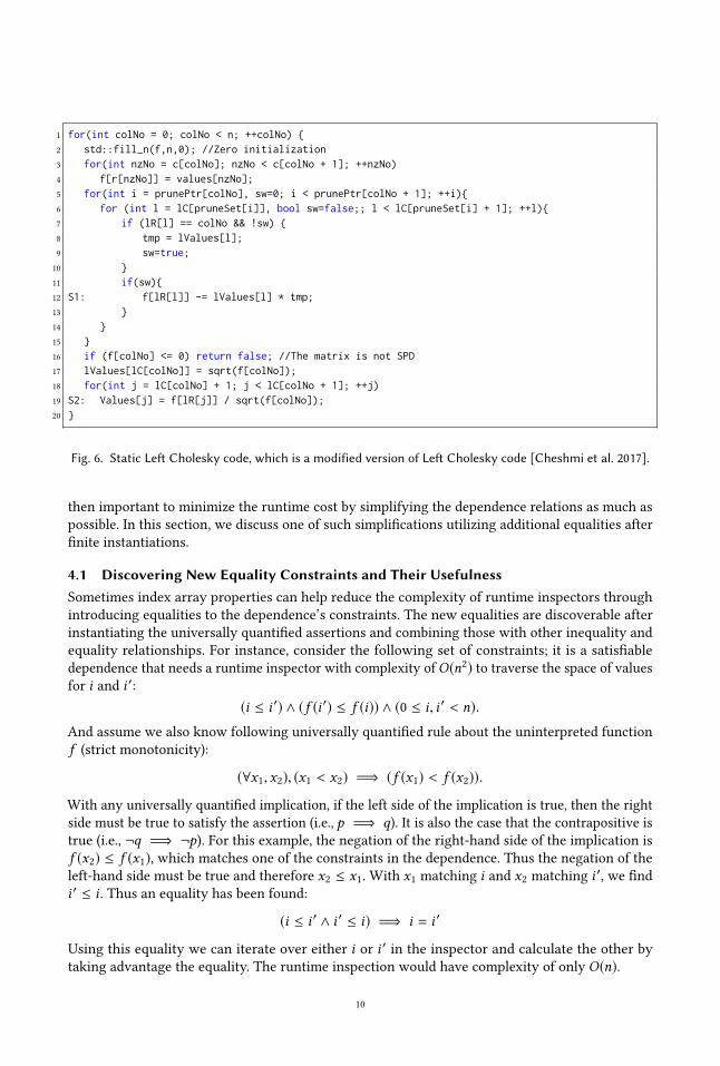
Fig. 6. Static Left Cholesky code, which is a modified version of Left Cholesky code [Cheshmi et al. 2017].
then important to minimize the runtime cost by simplifying the dependence relations as much as
possible. In this section, we discuss one of such simplifications utilizing additional equalities after
finite instantiations.
4.1 Discovering New Equality Constraints and Their UsefulnessSometimes index array properties can help reduce the complexity of runtime inspectors through
introducing equalities to the dependence’s constraints. The new equalities are discoverable after
instantiating the universally quantified assertions and combining those with other inequality and
equality relationships. For instance, consider the following set of constraints; it is a satisfiable
dependence that needs a runtime inspector with complexity ofO(n2) to traverse the space of valuesfor i and i ′:
(i ≤ i ′) ∧ (f (i ′) ≤ f (i)) ∧ (0 ≤ i, i ′ < n).And assume we also know following universally quantified rule about the uninterpreted function
f (strict monotonicity):
(∀x1,x2), (x1 < x2) =⇒ (f (x1) < f (x2)).
With any universally quantified implication, if the left side of the implication is true, then the right
side must be true to satisfy the assertion (i.e., p =⇒ q). It is also the case that the contrapositive is
true (i.e., ¬q =⇒ ¬p). For this example, the negation of the right-hand side of the implication is
f (x2) ≤ f (x1), which matches one of the constraints in the dependence. Thus the negation of the
left-hand side must be true and therefore x2 ≤ x1. With x1 matching i and x2 matching i ′, we findi ′ ≤ i . Thus an equality has been found:
(i ≤ i ′ ∧ i ′ ≤ i) =⇒ i = i ′
Using this equality we can iterate over either i or i ′ in the inspector and calculate the other by
taking advantage the equality. The runtime inspection would have complexity of only O(n).
10
4.2 Finding Equalities Example: Left CholeskyFor a more realistic example from one of the benchmarks used in the evaluation, consider a maybe
satisfiable dependence from our Static Left Cholesky shown in Figure 6. Following dependence is
coming from a read in S1 (lValues[l]), and a write in S2 (lValues[j]):
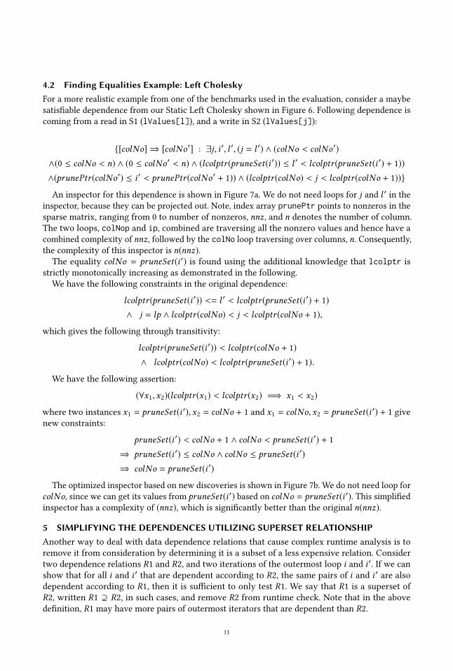
An inspector for this dependence is shown in Figure 7a. We do not need loops for j and l ′ in the
inspector, because they can be projected out. Note, index array prunePtr points to nonzeros in the
sparse matrix, ranging from 0 to number of nonzeros, nnz, and n denotes the number of column.
The two loops, colNop and ip, combined are traversing all the nonzero values and hence have a
combined complexity of nnz, followed by the colNo loop traversing over columns, n. Consequently,the complexity of this inspector is n(nnz).The equality colNo = pruneSet(i ′) is found using the additional knowledge that lcolptr is
strictly monotonically increasing as demonstrated in the following.
We have the following constraints in the original dependence:
The optimized inspector based on new discoveries is shown in Figure 7b. We do not need loop for
colNo, since we can get its values from pruneSet(i ′) based on colNo = pruneSet(i ′). This simplified
inspector has a complexity of (nnz), which is significantly better than the original n(nnz).
5 SIMPLIFYING THE DEPENDENCES UTILIZING SUPERSET RELATIONSHIPAnother way to deal with data dependence relations that cause complex runtime analysis is to
remove it from consideration by determining it is a subset of a less expensive relation. Consider
two dependence relations R1 and R2, and two iterations of the outermost loop i and i ′. If we canshow that for all i and i ′ that are dependent according to R2, the same pairs of i and i ′ are alsodependent according to R1, then it is sufficient to only test R1. We say that R1 is a superset of
R2, written R1 ⊇ R2, in such cases, and remove R2 from runtime check. Note that in the above
definition, R1 may have more pairs of outermost iterators that are dependent than R2.
(b) Inspector with an additional equality: colNo =pruneSet(i ′).
Fig. 7. Inspector pseudo-code for dependence constraints in Section 4.2, before and after utilizing indexarray properties to add new equalities. We obtain the equality colNo = pruneSet(i ′) using the properties asdescribed in Section 4.2. Notice how this equality is used to remove loop iterating over i in Line 3.
1 for (i = 0; i < n; i++) {2 S1: val[colPtr[i]] = sqrt(val[colPtr[i]]);3
4 for (m = colPtr[i] + 1; m < colPtr[i+1]; m++)5 S2: val[m] = val[m] / val[colPtr[i]];6
7 for (m = colPtr[i] + 1; m < colPtr[i+1]; m++)8 for (k = colPtr[rowIdx[m]] ; k < colPtr[rowIdx[m]+1]; k++)9 for ( l = m; l < colPtr[i+1] ; l++)10 if (rowIdx[l] == rowIdx[k] && rowIdx[l+1] <= rowIdx[k])11 S3: val[k] -= val[m]* val[l];12 }
Fig. 8. Incomplete Cholesky0 code from SparseLib++ [Pozo et al. 1996]. Some variable names have beenchanged. The arrays col and row are to represent common colPtr, and rowIdx in CSC format.
Taking advantage of this redundancy can result in lower complexity runtime analysis. As an
example, consider the Incomple Cholesky code shown in Figure 8. In section, we refer to an
array access A at statement S as A@S for brevity. One of the dependence tests is between the
write val[k]@S3 and the read val[m]@S3. This test is redundant with the test between the write
val[k]@S3 and the read val[m]@S2. This is because an iteration of the i loop that make the read
from val[m] in S3 is guaranteed to access the same memory location while executing the loop
surrounding S2. Thus, the more expensive check between accesses in S3 can be removed.
In this section, we describe our approach to identify redundant dependence relations. The key
challenge is to determine superset relations between two dependence tests involving uninterpreted
functions. We present two approaches that cover important cases, and discuss possible extensions.
5.1 Trivial Superset RelationsGiven a polyhedral dependence relation, it is easy to characterize the pairs of loop iterations that
are dependent. All the indices that do not correspond to the loop iterators in question can be
projected out to obtain the set of dependent iterations. These sets can be compared to determine if
a dependence test is subsumed by another. In principle, this is what we do to check if a dependence
relation is redundant with another. However, dependence relations from sparse codes may have
variables passed as parameters to uninterpreted functions. Such variables cannot be projected out.
12
Thus, we employ an approach based on similarities in the constraint systems. The trivial case is
when the dependence relation R1 is expressed with a subset of constraints in another relation R2. Ifthis is the case, then R1 can be said to be superset equal to R2.We illustrate this approach with the earlier example from Incomplete Cholesky. We take two
dependence relations, R1 between val[k]@S3 and val[m]@S2, and R2 between val[k]@S3 and
val[m]@S3. The relations—omitting the obviously common constraints for val[k]@S3—are:
R1 = {[i,m,k, l] → [i ′,m′] : k =m′ ∧ i < i ′ ∧ 0 ≤ i ′ < n ∧ col(i ′) + 1 ≤ m′ < col(i ′ + 1)}R2 = {[i,m,k, l] → [i ′,m′,k ′, l ′] : k =m′ ∧ i < i ′ ∧ 0 ≤ i ′ < n ∧ col(i ′) + 1 ≤ m′ < col(i ′ + 1)
We use three software packages to automate applying methods described in this paper: IEGenLib
library [Strout et al. 2016], ISL library [Verdoolaege 2018], and CHILL compiler framework [chi
2018]. CHiLL is a source-to-source compiler framework for composing and applying high level
loop transformations to improve the performance of nested loop written in C. We utilize CHILL to
extracted the dependence relations from the benchmarks. ISL is a library for manipulating integer
sets and relations that only contain affine constraints. It can act as a constraint solver by testing
the emptiness of integer sets. It is also equipped with a function for detecting equalities in sets
and relations. ISL does not support uninterpreted functions, and thus cannot directly represent
the dependence constraints in sparse matrix code. IEGenLib is a set manipulation library that
can manipulate integer sets/relations that contain uninterpreted function symbols. The IEGenLib
library utilizes ISL for some of its fundamental functionalities. We have implemented detecting
unsatisfiable dependences and finding the equalities utilizing the IEGenLib and ISL libraries.
The following briefly describes how the automation works. First, we extract the dependence
relations utilizing CHILL, and store them in IEGenLib. The user defined index array properties are
also stored in IEGenLib. Next, the instantiation procedure is carried out in IEGenLib. Then inside
IEGenLib, the uninterpreted functions are removed by replacing each call with a fresh variable, and
adding constraints that encode functional consistency [Kroening and Strichman 2016, Chapter 4].
Next, ISL can be utilized by IEGenLib to find the empty sets, i.e, unsatisfiable relations. Additionally,
equality detection is available as one of many operations supported by ISL The finite instantiations
described in Section 3.4 are intersections of the assertions with the dependence relation.
6.2 OptimizationA straightforward approach to implementing the procedure in Section 3.4 would be to take the
quantifier-free formula resulting from instantiation, replace the uninterpreted functions, and
directly pass it to ISL. However, this approach does not scale to large numbers of instantiations.
An instantiated assertion is encoded as a union of two constraints (¬p ∨ q). Given n instantiations,
this approach introduces 2ndisjunctions to the original relation, although many of the clauses
may be empty. In some of our dependence relations, the value of n may exceed 1000, resulting
in a prohibitively high number of disjunctions. We have observed that having more than 100
instantiations causes ISL to start having scalability problems.
14
We apply an optimization to avoid introducing disjunctions when possible. Given a set of
instantiations, the optimization adds the instantiations to the dependence relation in two phases.
The first phase only instantiates those that do not introduce disjunctions to the dependence relation.
During this phase, we check if the antecedent is already part of the dependence constraint, and
thus is always true. If this is the case, then q can be directly added to the dependence relation. We
also perform the same for ¬q =⇒ ¬p and add ¬p to the dependence relation if ¬q is always true.
The second phase adds the remaining instantiations that introduce disjunctions. This optimization
helps reducing the cost of dependence testing in two ways: (1) if the relation is unsatisfiable after
the first phase, disjunctions are completely avoided; and (2) the second phase only instantiates the
remainder, reducing the number of disjunctions.
If the dependence relation remains non-empty after the second phase, then the relation is checked
at runtime. All equalities in a relation is made explicit before inspector code generation with ISL so
that the code generator can take advantage of the equalities to simplify the generated code.
6.3 Contrasting SMT with ISLSMT solvers are specialized for solving satisfiability problems expressed as a combination of
background theories. ISL is a library for manipulating integer sets, and is specialized for the theory
of Presburger arithmetic over integers.
The finite instantiation in Section 3.4 is well-suited for SMT solvers. In fact, SMT solvers are
equipped with their own instantiation algorithms that also work well for our dependence relations.
However, SMT solvers do not provide any equality relationships they might derive while answering
the satisfiability question. Although it is possible to use SMT solvers to test if an equation is true for
a set of constraints, we cannot search for an equation given the constraints (unless all candidates
are enumerated—but there are infinite candidates in general).
For our implementation, the choice was between adding finite instantiation to ISL or adding
equality detection to SMT solvers. We have chosen the former option as it seemed simpler to do,
and also because we are more familiar with ISL.
7 EVALUATION OF UNSATISFIABILITY AND SIMPLIFICATION APPROACHESIn this section, we study the impact of our approach of utilizing domain information about index
arrays on the data dependence analysis of eight sparse kernels. Our approach may help data depen-
dence analysis in three ways: (1) The runtime check can be completely removed if the dependences
are proven unsatisfiable; (2) Deriving equalities from instantiated universally quantified assertions
about domain information can simplify dependences and reduce respected runtime check complex-
ity; and (3) Reducing all maybe satisfiable relations of a given code to a set of dependence relations
that encompass all potential dependences. We do this by finding relations that are superset equal
of other relations. This can discard even more dependence relations that potentially might need
expensive runtime checks.
We first describe the suite of numerical kernels that we have compiled to evaluate our approach.
Then we evaluate the impact of each step in our approach, from the relevance of the index property
assertions to the simplification using superset relations. Finally, we report the complexity of
inspectors with and without our proposed simplifications.
7.1 Numerical Algorithms in BenchmarkWe have included some of the most popular sparse kernels in a benchmark suite: (1) The Cholesky
factorization, Incomplete LU0 and Incomplete Cholesky0, and the sparse triangular solver, which
are commonly used in direct solvers and as preconditioners in iterative solvers; (2) sparse matrix
vector multiplication, and Gauss-Seidel methods, which are often used in iterative solvers. Table 1
15
Table 1. The benchmark suite used in this paper. The suite includes the fundamental blocksin several applications. The suite is also selected to cover both static index arrays, such asGauss-Seidel, and dynamic index arrays, such as Left Cholesky. The modification columnshows the type of modification applied to the original code.
Algorithm name Format Library source Mod.
Gauss-Seidel solver CSR Intel MKL [Wang et al. 2014] None
Gauss-Seidel solver BCSR Intel MKL [Wang et al. 2014] None
Incomplete LU CSR Intel MKL [Wang et al. 2014] None
Incomplete Cholesky CSC and CSR SparseLib++ [Pozo et al. 1996] None
Forward solve CSC Sympiler [Cheshmi et al. 2017] None
Forward solve CSR [Vuduc et al. 2002] None
Sparse MV Multiply CSR Common None
Static Left Cholesky CSC Sympiler [Cheshmi et al. 2017] Pa+ R
b
aPrivatization of temporary arrays
bRemoval of dynamic index array updates
summarizes the benchmarks indicating which library each algorithm came from and how the
benchmark compares with the implementations in existing libraries.
We modified onr of the benchmarks, left Cholesky, to make temporary arrays privatizable and to
remove dynamic index array updates so that the compiler can analyze the sparse code.
Left Cholesky: This code has following changes compared to a more common implementation
in CSparse [Davis 2006]: (i) Privatization of temporary arrays: We analyzed dependences between
reads and writes to temporary arrays to detect privatizable arrays. This can be challenging for a
compiler to do with sparse codes since accesses to these arrays are irregular. We set the values of
these arrays to zero at the beginning of each loop so a compiler could identify them as privatizable.
(ii) Removal of dynamic index array updates: Previous data dependence analysis work focuses on
cases where index arrays are not updated. However, in some numerical codes, updating index
arrays is a common optimization. We refer to this as dynamic index array updates, and it usually
occurs when the nonzero structure of an output matrix is modified in the sparse code during
the computation. This would make dependence analysis very complicated for the compiler. We
removed dynamic index arrays by partially decoupling symbolic analysis from the numerical code
in these benchmarks. Symbolic analysis here refers to terminology used in the numerical computing
community. Symbolic analysis uses the nonzero pattern of the matrix to determine computation
patterns and the sparsity of the resulting data. To remove dynamic index array updates, we decouple
symbolic analysis from the code similar to the approach used by [Cheshmi et al. 2017].
Performance Impact: The changes made to Left Cholesky do not have a noticeable effect on
the code performance. Based on our experiments using five matrices1from the Florida Sparse
Matrix Collection [Davis and Hu 2011] the performance cost of these modifications is on average
less than 10% than the original code.
7.2 Relevance of Index Array PropertiesWe have extracted the constraints to test for dependences that are carried by the outermost loop for
the sparse matrix codes in Table 1. A total of 124 data dependences relations were collected from
the benchmarks. Of those 124, only 83 of them were unique, the repetition coming from accesses
1Problem1, rdb450l, wang2, ex29, Chebyshev2
16
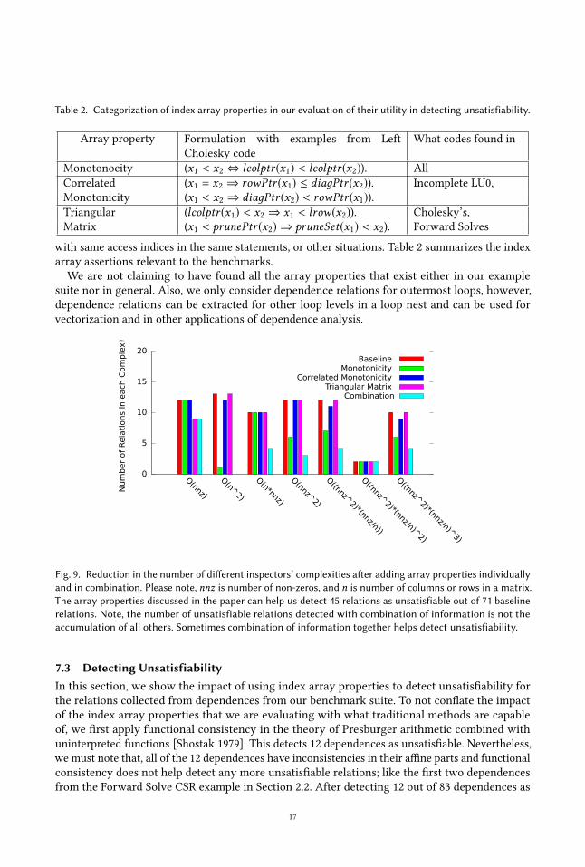
Table 2. Categorization of index array properties in our evaluation of their utility in detecting unsatisfiability.
Array property Formulation with examples from Left
with same access indices in the same statements, or other situations. Table 2 summarizes the index
array assertions relevant to the benchmarks.
We are not claiming to have found all the array properties that exist either in our example
suite nor in general. Also, we only consider dependence relations for outermost loops, however,
dependence relations can be extracted for other loop levels in a loop nest and can be used for
vectorization and in other applications of dependence analysis.
0
5
10
15
20
O(nnz)
O(n^2)
O(n*nnz)
O(nnz^2)
O((nnz^2)*(nnz/n))
O((nnz^2)*(nnz/n)^
2)
O((nnz^2)*(nnz/n)^
3)
Num
ber
of
Rela
tions
in e
ach
Com
ple
xit
y
Baseline Monotonicity
Correlated Monotonicity Triangular Matrix
Combination
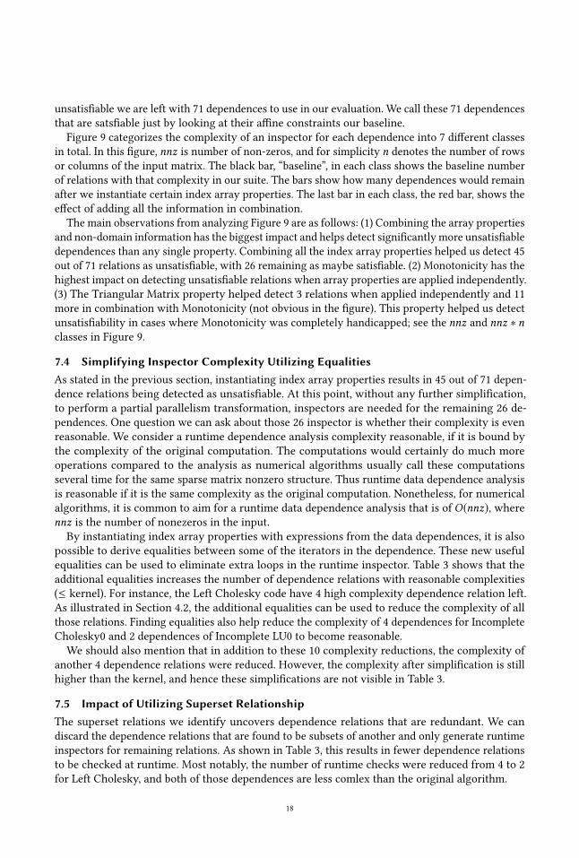
Fig. 9. Reduction in the number of different inspectors’ complexities after adding array properties individuallyand in combination. Please note, nnz is number of non-zeros, and n is number of columns or rows in a matrix.The array properties discussed in the paper can help us detect 45 relations as unsatisfiable out of 71 baselinerelations. Note, the number of unsatisfiable relations detected with combination of information is not theaccumulation of all others. Sometimes combination of information together helps detect unsatisfiability.
7.3 Detecting UnsatisfiabilityIn this section, we show the impact of using index array properties to detect unsatisfiability for
the relations collected from dependences from our benchmark suite. To not conflate the impact
of the index array properties that we are evaluating with what traditional methods are capable
of, we first apply functional consistency in the theory of Presburger arithmetic combined with
uninterpreted functions [Shostak 1979]. This detects 12 dependences as unsatisfiable. Nevertheless,
we must note that, all of the 12 dependences have inconsistencies in their affine parts and functional
consistency does not help detect any more unsatisfiable relations; like the first two dependences
from the Forward Solve CSR example in Section 2.2. After detecting 12 out of 83 dependences as
17
unsatisfiable we are left with 71 dependences to use in our evaluation. We call these 71 dependences
that are satsfiable just by looking at their affine constraints our baseline.
Figure 9 categorizes the complexity of an inspector for each dependence into 7 different classes
in total. In this figure, nnz is number of non-zeros, and for simplicity n denotes the number of rows
or columns of the input matrix. The black bar, “baseline”, in each class shows the baseline number
of relations with that complexity in our suite. The bars show how many dependences would remain
after we instantiate certain index array properties. The last bar in each class, the red bar, shows the
effect of adding all the information in combination.
The main observations from analyzing Figure 9 are as follows: (1) Combining the array properties
and non-domain information has the biggest impact and helps detect significantly more unsatisfiable
dependences than any single property. Combining all the index array properties helped us detect 45
out of 71 relations as unsatisfiable, with 26 remaining as maybe satisfiable. (2) Monotonicity has the
highest impact on detecting unsatisfiable relations when array properties are applied independently.
(3) The Triangular Matrix property helped detect 3 relations when applied independently and 11
more in combination with Monotonicity (not obvious in the figure). This property helped us detect
unsatisfiability in cases where Monotonicity was completely handicapped; see the nnz and nnz ∗ nclasses in Figure 9.
7.4 Simplifying Inspector Complexity Utilizing EqualitiesAs stated in the previous section, instantiating index array properties results in 45 out of 71 depen-
dence relations being detected as unsatisfiable. At this point, without any further simplification,
to perform a partial parallelism transformation, inspectors are needed for the remaining 26 de-
pendences. One question we can ask about those 26 inspector is whether their complexity is even
reasonable. We consider a runtime dependence analysis complexity reasonable, if it is bound by
the complexity of the original computation. The computations would certainly do much more
operations compared to the analysis as numerical algorithms usually call these computations
several time for the same sparse matrix nonzero structure. Thus runtime data dependence analysis
is reasonable if it is the same complexity as the original computation. Nonetheless, for numerical
algorithms, it is common to aim for a runtime data dependence analysis that is of O(nnz), wherennz is the number of nonezeros in the input.
By instantiating index array properties with expressions from the data dependences, it is also
possible to derive equalities between some of the iterators in the dependence. These new useful
equalities can be used to eliminate extra loops in the runtime inspector. Table 3 shows that the
additional equalities increases the number of dependence relations with reasonable complexities
(≤ kernel). For instance, the Left Cholesky code have 4 high complexity dependence relation left.
As illustrated in Section 4.2, the additional equalities can be used to reduce the complexity of all
those relations. Finding equalities also help reduce the complexity of 4 dependences for Incomplete
Cholesky0 and 2 dependences of Incomplete LU0 to become reasonable.
We should also mention that in addition to these 10 complexity reductions, the complexity of
another 4 dependence relations were reduced. However, the complexity after simplification is still
higher than the kernel, and hence these simplifications are not visible in Table 3.
7.5 Impact of Utilizing Superset RelationshipThe superset relations we identify uncovers dependence relations that are redundant. We can
discard the dependence relations that are found to be subsets of another and only generate runtime
inspectors for remaining relations. As shown in Table 3, this results in fewer dependence relations
to be checked at runtime. Most notably, the number of runtime checks were reduced from 4 to 2
for Left Cholesky, and both of those dependences are less comlex than the original algorithm.
18
Table 3. Effect of simplifications based additional equalities (Section 4) and redundancy elimination (Section 5)on the remaining 26 maybe satisfiable dependences for each code in the benchmark. The Total columns showthe number of dependence relations that needs to be checked at runtime. The ≤ kernel columns show thenumber of such tests that have the same or lower complexity than the kernel. Equality Impact is the numbersafter using additional equalities, reducing the number of high complexity checks. Supserset Impact is thecomposed effect of using supserset relations after adding equalities, reducing the total number of checks.
Kernel name Remaining satisfiables Equality Impact Superset Impact
As discussed in Section 5, the superset relation may reveal that a relation is redundant being
subset of another relation with lower complexity. The Incomplete Cholesky kernel were left with
4 expensive relations even after adding equalities. As you can see in Table 3, these relations are
removed from runtime checks by identifying the superset relations. For Incomplete Cholesky
kernel, we have found 2 relations with less than orginal algorithm complexity to be superset of all
the dependences that we need to have a runtime check for. The composed effect of our proposed
technique reduces the inspector cost to 2 or fewer inexpensive tests for all of our kernels, except
for the Incomplete LU.
7.6 Putting It All TogetherWe have presented a series of techniques to simplify dependence relations with the main moti-
vation being automatic generation of efficient inspector code. Our approach aims to simplify the
dependence relations starting from array properties that can be succinctly specified by the experts.
We show that the array properties can be used to automatically disprove a large number of potential
dependences, as well as reduce the complexity of remaining dependences. Combined with a method
for detecting redundancies in dependence tests, we are able to generate efficient inspectors.
Table 4 summarizes the impact of our proposed approach on inspector complexity. It is interesting
to note that Incomplete LU0 is the only kernel left with expensive inspector (more complex than
kernel). This case is discussed further in Section 7.7.
7.7 Discussion: LimitationsTable 4 demonstrates that our method significantly reduces both the number of runtime checks
and their complexity. Nonetheless, our approach is not free of limitations, which are discussed in
this section.
Two of the original kernels include dynamic index arrays and temporary arrays that require
privatization. As discussed in Section 7.1, these kernels can be preprocessed such that it can be
accepted by our compiler. This preprocessing is currently done manually.
Using the associativity of reductions is important for Forward Solve CSC and Incomplete
Cholesky0. We do not automate the reduction detection in this paper, as it is a complex task
19
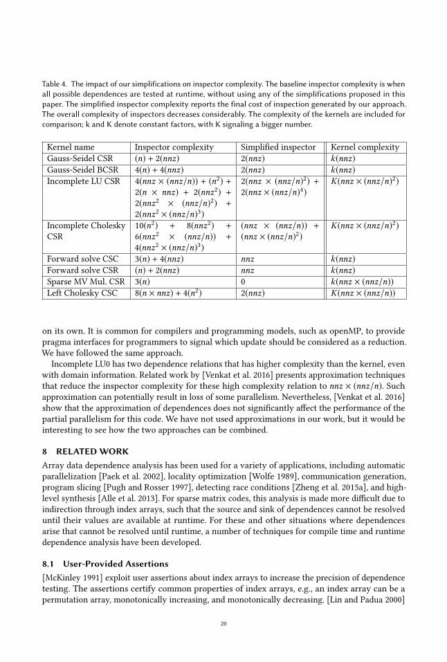
Table 4. The impact of our simplifications on inspector complexity. The baseline inspector complexity is whenall possible dependences are tested at runtime, without using any of the simplifications proposed in thispaper. The simplified inspector complexity reports the final cost of inspection generated by our approach.The overall complexity of inspectors decreases considerably. The complexity of the kernels are included forcomparison; k and K denote constant factors, with K signaling a bigger number.
Kernel name Inspector complexity Simplified inspector Kernel complexity
on its own. It is common for compilers and programming models, such as openMP, to provide
pragma interfaces for programmers to signal which update should be considered as a reduction.
We have followed the same approach.
Incomplete LU0 has two dependence relations that has higher complexity than the kernel, even
with domain information. Related work by [Venkat et al. 2016] presents approximation techniques
that reduce the inspector complexity for these high complexity relation to nnz × (nnz/n). Suchapproximation can potentially result in loss of some parallelism. Nevertheless, [Venkat et al. 2016]
show that the approximation of dependences does not significantly affect the performance of the
partial parallelism for this code. We have not used approximations in our work, but it would be
interesting to see how the two approaches can be combined.
8 RELATEDWORKArray data dependence analysis has been used for a variety of applications, including automatic
parallelization [Paek et al. 2002], locality optimization [Wolfe 1989], communication generation,
program slicing [Pugh and Rosser 1997], detecting race conditions [Zheng et al. 2015a], and high-
level synthesis [Alle et al. 2013]. For sparse matrix codes, this analysis is made more difficult due to
indirection through index arrays, such that the source and sink of dependences cannot be resolved
until their values are available at runtime. For these and other situations where dependences
arise that cannot be resolved until runtime, a number of techniques for compile time and runtime
dependence analysis have been developed.
8.1 User-Provided Assertions[McKinley 1991] exploit user assertions about index arrays to increase the precision of dependence
testing. The assertions certify common properties of index arrays, e.g., an index array can be a
permutation array, monotonically increasing, and monotonically decreasing. [Lin and Padua 2000]
20
present a compile time analysis for determining index array properties, such as monotonicity. They
use the analysis results for parallelization of sparse matrix computations.
Our approach also uses these assertions, but in addition we use more domain-specific assertions
and provide a way to automate the general use of such assertions. In this paper, the idea of applying
constraint instantiation of universally quantified constraints as is done in SMT solvers to find
unsatisfactory dependences is novel and the assertions about index arrays we use are more general.
8.2 Proving Index Arrays Satisfy the AssertionsIn this work, we assume that the assertions provided by the programmer is correct. It is useful to
verify the user-provided assertions by analyzing the code that constructs the sparse matrix data
structures. There is a large body of work in abstract interpretation that address this problem.
The major challenge in verifying the assertion about programs that manipulate arrays is the
trade-off between scalability and precision. When there is a large number of updates to an array,
keeping track of individual elements do not scale, but approximating the whole array as a single
summary significantly degrades the precision. Many techniques to verify/infer important properties
about array contents from programs have been developed, e.g., [Cousot et al. 2011; Gopan et al.
2005; Halbwachs and Péron 2008].
In the work by [Henzinger et al. 2010], the authors present an approach for inferring shape
invariants for matrices. While their work does not deal with sparse matrices and index arrays, it may
help generate domain-specific assertions that we could employ to show that the data dependences
are unsatisfiable.
The main subject of our work - dependence tests - does not involve array updates, since all the
index arrays, which alter the control-flow and indexing of the data arrays, are not updated. This
makes the verification of the assertions a closely related but orthogonal problem, which we do not
address in this paper.
8.3 More GeneralQuantifier Elimination TechniquesThe area of SMT-solving is advancing at a significant pace; the webpage for SMT-COMP
2provides
a list of virtually all actively developed solvers, and how they fared in each theory category. As
these solvers are moving into a variety of domains, quantifier instantiation and elimination has
become a topic of central interest. Some of the recent work in this area are: E-matching [Moura
and Bjørner 2007], Model-Based [Ge and de Moura 2009], Conflict-Based [Reynolds et al. 2014],
and Counter-Example Guided [Reynolds et al. 2015].
These efforts make it clear that quantifier instantiation is challenging, and is an area of active
development. SMT solvers often rely on heuristic-driven instantiations to show unsat for difficult
problems. In this context, our work can be viewed as heuristic instantiation where the heuristic is
inspired by decidable fragments of the array theory.
Dependence constraints with universally quantified assertions are related to the first order
theory fragments described by [Bradley et al. 2006] as undecidable extensions to their array theory
fragment. However, [Löding et al. 2017] claim that the proofs for undecidability of extension
theories by [Bradley et al. 2006] are incorrect, and declare their decidability status as an open
problem. Regardless of whether the theory fragment that encompasses our dependence constraints
is decidable or not following is true: if we soundly prove that a relation is unsatisfiable just with
compile time information, the unsatisfiability applies in general, and having runtime information
would not change anything. However, if a dependence detected to be satisfiable just with compile
time information, we need to have runtime tests to see if it is actually satisfiable given runtime
information, and even if it is, run time tests would determine for what values the dependence holds.
8.4 Dependence Analysis for Full ParallelizationSome compilation techniques have been developed to extend the dependence analysis to sparse,
or non-affine programs [Benabderrahmane et al. 2010]. These techniques extend to non-affine
programs of various forms: while loops, polynomial expressions, function calls, data-dependent
conditions, and indirection arrays. The outcome of such analysis is often an approximation, which
is quite pessimistic for sparse computations involving indirection arrays. The focus of our work is
not to identify (approximated) dependences, but to reduce the cost of runtime dependence checks
by disproving potential dependences as much as possible at compile-time.
The work by [Pugh and Wonnacott 1998] also formulate the problem in the theory of Presburger
sets with uninterpreted functions. However, they only allow affine expressions of unquantified
variables as indexing expressions to the function symbols, excluding some of the examples in this
paper. They propose an analysis to identify conditions for a dependence to exist through the use
of gist operator that simplifies the constraint system given its context. The result of this analysis
may involve uninterpreted functions, and can be used to query the programmer for their domain
knowledge. This is an interesting direction of interaction that complements our work.
Several runtime approaches focus on identifying loops we denoted fully parallel whose iterationsare independent and can safely execute in parallel [Barthou et al. 1997; Moon and Hall 1999; Pugh
and Wonnacott 1998] or speculatively execute in parallel while testing safety [Rauchwerger and
Padua 1999].
8.5 Dependence Analysis for Wavefront ParallelizationFor sparse codes, even when loops carry dependences, the dependences themselves may be sparse,
and it may be possible to execute some iterations of the loop in parallel (previously denoted
partially parallel. The parallelism is captured in a task graph, and typically executed as a parallel
wavefront. A number of prior works write specialized code to derive this task graph as part of
their application [Bell and Garland 2009; Park et al. 2014a,b; Rauchwerger et al. 1995a; Saltz et al.
1991; Zhuang et al. 2009] or with kernel-specific code generators [Byun et al. 2012]. For example,
Saltz and Rothbergs worked on manual parallelization of sparse triangular solver codes in the
1990s [Rothberg and Gupta 1992; Saltz 1990]. There is also more recent work on optimizing sparse
triangular solver NVIDIA GPUs and Intel’s multi-core CPUs [Rennich et al. 2016; Wang et al. 2014].
Even though these manual optimizations have been successful at achieving high performance in
some cases, significant programmer effort has to be invested for each of these codes and automating
these parallelization strategies can significantly reduce this effort.
Other approaches automate the generation of inspectors that find task-graph, wavefront or partial
parallelism. [Rauchwerger et al. 1995b] and others [Huang et al. 2013] have developed efficient and
parallel inspectors that maintain lists of iterations that read and write each memory location. By
increasing the number of dependences found unsatisfiable, the approach presented in this paper
reduces the number of memory accesses that would need to be tracked. For satisfiable dependences,
there is a tradeoff between inspecting iteration space dependences versus maintaining data for each
memory access. That choice could bemade at runtime. There are also other approaches for automatic
generation of inspectors that have looked at simplifying the inspector by finding equalities, using
approximation, parallelizing the inspector, and applying point-to-point synchronization to the
executor [Venkat et al. 2016].
22
8.6 Algorithm-Specific Data Dependence AnalysisAn algorithm-specific approach to represent data dependences and optimize memory usage of
sparse factorization algorithms such as Cholesky [Pothen and Toledo 2004] uses an eliminationtree, but to the best of our knowledge, this structure is not derived automatically from source code.
When factorizing a column of a sparse matrix, in addition to nonzero elements of the input matrix
new nonzero elements, called fill-in, might be created. Since the sparse matrices are compressed for
efficiency, the additional fills during factorization make memory allocation ahead of factorization
difficult. The elimination tree is used to predict the sparsity pattern of the L factor ahead of
factorization so the size of the factor can be computed [Coleman et al. 1986] or predicted [Gilbert
1994; Gilbert and Ng 1993], and captures a potential parallel schedule of the tasks. Prior work
has investigated the applicability of the elimination tree for dependence analysis for parallel
implementation [George et al. 1989; Gilbert and Schreiber 1992; Hénon et al. 2002; Hogg et al. 2010;
Karypis and Kumar 1995; Pothen and Sun 1993; Rennich et al. 2016; Schenk and Gärtner 2002;
Zheng et al. 2015b]. Some techniques such as [George et al. 1989; Hénon et al. 2002; Pothen and
Sun 1993] use the elimination tree for static scheduling while others use it for runtime scheduling.
9 CONCLUSIONIn this paper, we present an automated approach for showing sparse code data dependences
are unsatisfiable or if not reducing the complexity for later runtime analysis. Refuting a data
dependence brings benefits to many areas of sparse matrix code analysis, including verification
and loop optimizations such as parallelization, pipelining, or tiling by completely eliminating the
high runtime costs of deploying runtime dependence checking. Additionally, when a dependence
remains satisfiable, our approach of performing constraint instantiation within the context of the
Integer Set Library (ISL) enables equalities and subset relationships to be derived that simplify
the runtime complexity of inspectors for a case study with wavefront parallelism. Parallelization
of these sparse numerical methods is an active research area today, but one where most current
approaches requiremanual parallelization. It is also worth noting that without inspector complexity
reduction, most inspectors would timeout, thus underscoring the pivotal role of the work in this
paper in enabling parallelization and optimization of sparse codes. Our results are established over
71 dependences extracted from 8 sparse numerical methods.
REFERENCES2018. CTOP research group webpage at Utah. (2018). http://ctop.cs.utah.edu/ctop/?page_id=21
Mythri Alle, Antoine Morvan, and Steven Derrien. 2013. Runtime Dependency Analysis for Loop Pipelining in High-level
Synthesis. In Proceedings of the 50th Annual Design Automation Conference (DAC ’13). ACM, New York, NY, USA, Article
Simone Atzeni, Ganesh Gopalakrishnan, Zvonimir Rakamaric, Dong H. Ahn, Ignacio Laguna, Martin Schulz, Gregory L. Lee,
Joachim Protze, and Matthias S. Müller. 2016a. ARCHER: Effectively Spotting Data Races in Large OpenMP Applications.
In 2016 IEEE International Parallel and Distributed Processing Symposium, IPDPS 2016, Chicago, IL, USA, May 23-27, 2016.53–62. https://doi.org/10.1109/IPDPS.2016.68
S. Atzeni, G. Gopalakrishnan, Z. Rakamaric, D. H. Ahn, I. Laguna, M. Schulz, G. L. Lee, J. Protze, and M. S. MÃijller.
2016b. ARCHER: Effectively Spotting Data Races in Large OpenMP Applications. In 2016 IEEE International Parallel andDistributed Processing Symposium (IPDPS). 53–62. https://doi.org/10.1109/IPDPS.2016.68
Uptal Banerjee, David Gelernter, Alex Nicolau, and David Padua (Eds.). 1993. An Exact Method for Analysis of Value-basedArray Data Dependences. Springer-Verlag, London, UK.
Denis Barthou, Jean-François Collard, and Paul Feautrier. 1997. Fuzzy Array Dataflow Analysis. J. Parallel and Distrib.Comput. 40, 2 (1997), 210–226.
Ayon Basumallik and Rudolf Eigenmann. 2006. Optimizing irregular shared-memory applications for distributed-memory
systems. In Proceedings of the Eleventh ACM SIGPLAN Symposium on Principles and Practice of Parallel Programming.ACM Press, New York, NY, USA, 119–128.
Nathan Bell andMichael Garland. 2009. Implementing sparsematrix-vectormultiplication on throughput-oriented processors.
In SC ’09: Proceedings of the Conference on High Performance Computing Networking, Storage and Analysis. ACM, New
York, NY, USA, 1–11.
Mohamed-Walid Benabderrahmane, Louis-Noël Pouchet, Albert Cohen, and Cédric Bastoul. 2010. The Polyhedral Model Is
More Widely Applicable Than You Think. In Compiler Construction, Vol. LNCS 6011. Springer-Verlag, Berlin, Heidelberg.Aaron R. Bradley, Zohar Manna, and Henny B. Sipma. 2006. What’s Decidable About Arrays? Springer Berlin Heidelberg,
T. Brandes. 1988. The importance of direct dependences for automatic parallelism. In Proceedings of the InternationalConference on Supercomputing. ACM, New York, NY, USA, 407–417.
Jong-Ho Byun, Richard Lin, Katherine A. Yelick, and James Demmel. 2012. Autotuning Sparse Matrix-Vector Multiplicationfor Multicore. Technical Report. UCB/EECS-2012-215.
Matrix Codes by Decoupling Symbolic Analysis. In Proceedings of the International Conference for High PerformanceComputing, Networking, Storage and Analysis (SC ’17). ACM, New York, NY, USA, Article 13, 13 pages. https://doi.org/10.
1145/3126908.3126936
Thomas F Coleman, Anders Edenbrandt, and John R Gilbert. 1986. Predicting fill for sparse orthogonal factorization. Journalof the ACM (JACM) 33, 3 (1986), 517–532.
Patrick Cousot, Radhia Cousot, and Francesco Logozzo. 2011. A Parametric Segmentation Functor for Fully Automatic and
Scalable Array Content Analysis. In Proceedings of the 38th Symposium on Principles of Programming Languages (POPL’11). 105–118. https://doi.org/10.1145/1926385.1926399
Timothy A Davis. 2006. Direct methods for sparse linear systems. Vol. 2. Siam.
Timothy A Davis and Yifan Hu. 2011. The University of Florida sparse matrix collection. ACM Transactions on MathematicalSoftware (TOMS) 38, 1 (2011), 1.
Craig C. Douglas, Jonathan Hu, Markus Kowarschik, Ulrich Rüde, and Christian Weiß. 2000. Cache Optimization for
Structured and Unstructured Grid Multigrid. Electronic Transaction on Numerical Analysis (February 2000), 21–40.
Paul Feautrier. 1991. Dataflow Analysis of Array and Scalar References. International Journal of Parallel Programming 20, 1
(February 1991), 23–53.
Yeting Ge and Leonardo de Moura. 2009. Complete Instantiation for Quantified Formulas in Satisfiabiliby Modulo Theories.Springer Berlin Heidelberg, Berlin, Heidelberg, 306–320.
Alan George, Joseph WH Liu, and Esmond Ng. 1989. Communication results for parallel sparse Cholesky factorization on a
hypercube. Parallel Comput. 10, 3 (1989), 287–298.John R Gilbert. 1994. Predicting structure in sparse matrix computations. SIAM J. Matrix Anal. Appl. 15, 1 (1994), 62–79.John R Gilbert and Esmond G Ng. 1993. Predicting structure in nonsymmetric sparse matrix factorizations. In Graph theory
and sparse matrix computation. Springer, 107–139.John R Gilbert and Robert Schreiber. 1992. Highly parallel sparse Cholesky factorization. SIAM J. Sci. Statist. Comput. 13, 5
(1992), 1151–1172.
Denis Gopan, Thomas Reps, andMooly Sagiv. 2005. A Framework for Numeric Analysis of Array Operations. In Proceedings ofthe 32nd Symposium on Principles of Programming Languages (POPL ’05). 338–350. https://doi.org/10.1145/1040305.1040333
Peter Habermehl, Radu Iosif, and Tomáš Vojnar. 2008. What else is Decidable About Integer Arrays?. In Proceedings of the11th International Conference on Foundations of Software Science and Computational Structures (FOSSACS’08/ETAPS’08).474–489.
Nicolas Halbwachs and Mathias Péron. 2008. Discovering Properties About Arrays in Simple Programs. In Proceedings ofthe 29th Conference on Programming Language Design and Implementation (PLDI ’08). 339–348. https://doi.org/10.1145/
1375581.1375623
Pascal Hénon, Pierre Ramet, and Jean Roman. 2002. PASTIX: a high-performance parallel direct solver for sparse symmetric
positive definite systems. Parallel Comput. 28, 2 (2002), 301–321.Thomas A. Henzinger, Thibaud Hottelier, Laura Kovács, and Andrei Voronkov. 2010. Invariant and Type Inference for
Matrices. In Verification, Model Checking, and Abstract Interpretation, 11th International Conference, VMCAI 2010, Madrid,Spain, January 17-19, 2010. Proceedings. 163–179.
Jonathan D Hogg, John K Reid, and Jennifer A Scott. 2010. Design of a multicore sparse Cholesky factorization using DAGs.
SIAM Journal on Scientific Computing 32, 6 (2010), 3627–3649.
Jialu Huang, Thomas B. Jablin, Stephen R. Beard, Nick P. Johnson, and David I. August. 2013. Automatically exploiting
cross-invocation parallelism using runtime information. In CGO. 1–11.George Karypis and Vipin Kumar. 1995. A high performance sparse Cholesky factorization algorithm for scalable parallel
computers. In Frontiers of Massively Parallel Computation, 1995. Proceedings. Frontiers’ 95., Fifth Symposium on the. IEEE,140–147.
Daniel Kroening and Ofer Strichman. 2016. Decision Procedures: An Algorithmic Point of View (2nd ed.). Springer Berlin
Heidelberg.
Yuan Lin and David Padua. 2000. Compiler analysis of irregular memory accesses. In Proceedings of the ACM SIGPLANConference on Programming Language Design and Implementation, Vol. 35. ACM, New York, NY, USA, 157–168.
Christof Löding, P. Madhusudan, and Lucas Peña. 2017. Foundations for Natural Proofs and Quantifier Instantiation. Proc.ACM Program. Lang. 2, POPL, Article 10 (Dec. 2017), 30 pages. https://doi.org/10.1145/3158098
Kathryn McKinley. 1991. Dependence Analysis of Arrays Subscriptecl by Index Arrays. Technical Report TR91187. RiceUniversity.
Sungdo Moon and Mary W. Hall. 1999. Evaluation of Predicated Array Data-flow Analysis for Automatic Parallelization.
In Proceedings of the Seventh ACM SIGPLAN Symposium on Principles and Practice of Parallel Programming (PPoPP ’99).ACM, New York, NY, USA, 84–95. https://doi.org/10.1145/301104.301112
Leonardo Moura and Nikolaj Bjørner. 2007. Efficient E-Matching for SMT Solvers. In Proceedings of the 21st International Con-ference on Automated Deduction: Automated Deduction (CADE-21). 183–198. https://doi.org/10.1007/978-3-540-73595-3_13
Cosmin E. Oancea and Lawrence Rauchwerger. 2012. Logical inference techniques for loop parallelization. In Proceedings ofthe 33rd ACM SIGPLAN conference on Programming Language Design and Implementation (PLDI ’12). ACM, New York, NY,
USA, 509–520.
Yunheung Paek, Jay Hoeflinger, and David Padua. 2002. Efficient and Precise Array Access Analysis. ACM Trans. Program.Lang. Syst. 24, 1 (Jan. 2002), 65–109.
Jongsoo Park, Mikhail Smelyanskiy, Narayanan Sundaram, and Pradeep Dubey. 2014a. Sparsifying Synchronization for
High-Performance Shared-Memory Sparse Triangular Solver. In Proceedings of the 29th International Conference onSupercomputing - Volume 8488 (ISC 2014). Springer-Verlag New York, Inc., New York, NY, USA, 124–140.
Jongsoo Park, Mikhail Smelyanskiy, Karthikeyan Vaidyanathan, Alexander Heinecke, Dhiraj D. Kalamkar, Xing Liu, Md.
Mosotofa Ali Patwary, Yutong Lu, and Pradeep Dubey. 2014b. Efficient Shared-memory Implementation of High-
performance Conjugate Gradient Benchmark and Its Application to Unstructured Matrices. In Proc. Int. Conf. for HighPerformance Computing, Networking, Storage and Analysis (SC ’14). IEEE Press, Piscataway, NJ, USA, 945–955.
Alex Pothen and Chunguang Sun. 1993. A mapping algorithm for parallel sparse Cholesky factorization. SIAM Journal onScientific Computing 14, 5 (1993), 1253–1257.
Alex Pothen and Sivan Toledo. 2004. Elimination Structures in Scientific Computing. (2004).
Roldan Pozo, Karin Remington, and Andrew Lumsdaine. 1996. SparseLib++ v. 1.5 Sparse Matrix Class Library reference
guide. NIST Interagency/Internal Report (NISTIR)-5861 (1996).Bill Pugh and David Wonnacott. 1994. Nonlinear Array Dependence Analysis. Technical Report CS-TR-3372. Dept. of
Computer Science, Univ. of Maryland.
William Pugh and Evan Rosser. 1997. Iteration space slicing and its application to communication optimization. In Proceedingsof the 11th international conference on Supercomputing. ACM Press, 221–228.
William Pugh and David Wonnacott. 1995. Nonlinear Array Dependence Analysis. In Third Workshop on Languages,Compilers, and Run-Time Systems for Scalable Computers. Troy, New York.
William Pugh and DavidWonnacott. 1998. Constraint-Based Array Dependence Analysis. ACM Transactions on ProgrammingLanguages and Systems 20, 3 (1 May 1998), 635–678.
L. Rauchwerger, N. M. Amato, and D. A. Padua. 1995a. Run-Time Methods for Parallelizing Partially Parallel Loops. In
Proceedings of the ACM International Conference on Supercomputing (ICS). ACM, New York, NY, USA, 137–146.
Lawrence Rauchwerger, Nancy M. Amato, and David A. Padua. 1995b. A Scalable Method for Run-Time Loop Parallelization.
International Journal of Parallel Programming 23, 6 (1995), 537–576.
Lawrence Rauchwerger and David A. Padua. 1999. The LRPD Test: Speculative Run-Time Parallelization of Loops with
Mahesh Ravishankar, Roshan Dathathri, Venmugil Elango, Louis-Noël Pouchet, J. Ramanujam, Atanas Rountev, and P.
Sadayappan. 2015. Distributed Memory Code Generation for Mixed Irregular/Regular Computations. In Proceedings ofthe 20th ACM SIGPLAN Symposium on Principles and Practice of Parallel Programming (PPoPP 2015). ACM, New York, NY,
USA, 65–75. https://doi.org/10.1145/2688500.2688515
Steven C Rennich, Darko Stosic, and Timothy A Davis. 2016. Accelerating sparse Cholesky factorization on GPUs. ParallelComput. 59 (2016), 140–150.
Andrew Reynolds, Morgan Deters, Viktor Kuncak, Clark W. Barrett, and Cesare Tinelli. 2015. On Counterexample Guided
Quantifier Instantiation for Synthesis in CVC4. CoRR abs/1502.04464 (2015). http://arxiv.org/abs/1502.04464
Andrew Reynolds, Cesare Tinelli, and Leonardo de Moura. 2014. Finding Conflicting Instances of Quantified Formulas in
SMT. In Proceedings of the 14th Conference on Formal Methods in Computer-Aided Design (FMCAD ’14). Article 31, 8 pages.Edward Rothberg and Anoop Gupta. 1992. Parallel ICCG on a hierarchical memory multiprocessor - Addressing the
Silvius Rus, Jay Hoeflinger, and Lawrence Rauchwerger. 2003. Hybrid analysis: static & dynamic memory reference analysis.
International Journal Parallel Programming 31, 4 (2003), 251–283.
Joel H. Saltz. 1990. Aggregation Methods for Solving Sparse Triangular Systems on Multiprocessors. SIAM J. Sci. Stat.Comput. 11, 1 (Jan. 1990), 123–144. https://doi.org/10.1137/0911008
Joel H. Saltz, Ravi Mirchandaney, and Kay Crowley. 1991. Run-Time Parallelization and Scheduling of Loops. IEEE Trans.Comput. 40, 5 (1991), 603–612.
Olaf Schenk and Klaus Gärtner. 2002. Two-level dynamic scheduling in PARDISO: Improved scalability on shared memory
multiprocessing systems. Parallel Comput. 28, 2 (2002), 187–197.Robert E. Shostak. 1979. A Practical Decision Procedure for Arithmetic with Function Symbols. J. ACM 26, 2 (April 1979),
351–360. https://doi.org/10.1145/322123.322137
Kevin Streit, Johannes Doerfert, Clemens Hammacher, Andreas Zeller, and Sebastian Hack. 2015. Generalized Task
Michelle Mills Strout, Larry Carter, Jeanne Ferrante, and Barbara Kreaseck. 2004. Sparse Tiling for Stationary Iterative
Methods. International Journal of High Performance Computing Applications 18, 1 (February 2004), 95–114.
Michelle Mills Strout, Alan LaMielle, Larry Carter, Jeanne Ferrante, Barbara Kreaseck, and Catherine Olschanowsky. 2016.
An Approach for Code Generation in the Sparse Polyhedral Framework. Parallel Comput. 53, C (April 2016), 32–57.
Anand Venkat, Mahdi Soltan Mohammadi, Jongsoo Park, Hongbo Rong, Rajkishore Barik, Michelle Mills Strout, and Mary
Hall. 2016. Automating Wavefront Parallelization for Sparse Matrix Computations. In Proceedings of the InternationalConference for High Performance Computing, Networking, Storage and Analysis (SC ’16). IEEE Press, Piscataway, NJ, USA,
Sven Verdoolaege. 2010. isl: An integer set library for the polyhedral model. In Proceedings of the 3rd International Congresson Mathematical Software (ICMS ’10). 299–302.
Sven Verdoolaege. 2018. Integer Set Library: Manual. http://isl.gforge.inria.fr//manual.pdf
Richard Vuduc, Shoaib Kamil, Jen Hsu, Rajesh Nishtala, James W Demmel, and Katherine A Yelick. 2002. Automatic
performance tuning and analysis of sparse triangular solve. ICS.
Endong Wang, Qing Zhang, Bo Shen, Guangyong Zhang, Xiaowei Lu, Qing Wu, and Yajuan Wang. 2014. Intel math kernel
library. In High-Performance Computing on the Intel® Xeon Phi. Springer, 167–188.M. Wolfe. 1989. More Iteration Space Tiling. In Proceedings of the 1989 ACM/IEEE Conference on Supercomputing (Supercom-
puting ’89). ACM, New York, NY, USA, 655–664. https://doi.org/10.1145/76263.76337
M. Zheng, M. S. Rogers, Z. Luo, M. B. Dwyer, and S. F. Siegel. 2015a. CIVL: Formal Verification of Parallel Programs. In 201530th IEEE/ACM International Conference on Automated Software Engineering (ASE). 830–835. https://doi.org/10.1109/ASE.
2015.99
Ran Zheng, Wei Wang, Hai Jin, Song Wu, Yong Chen, and Han Jiang. 2015b. GPU-based multifrontal optimizing method
in sparse Cholesky factorization. In Application-specific Systems, Architectures and Processors (ASAP), 2015 IEEE 26thInternational Conference on. IEEE, 90–97.
Xiaotong Zhuang, A.E. Eichenberger, Yangchun Luo, K. O’Brien, and K. O’Brien. 2009. Exploiting Parallelism with
Dependence-Aware Scheduling. In International Conference on Parallel Architectures and Compilation Techniques (PACT).IEEE Computer Society, Los Alamitos, CA, USA, 193–202.