10th Pacific Symposium on Flow Visualization and Image ProcessingNaples, Italy, 15-18 June, 2015

Spatial and temporal distribution of a pulsed jet in cross-flow - Experimentalvalidation of mixing efficiency predictions by CFD

Stefan Puttinger1,*, Gijsbert Wierink1, Stefan Pirker1

1Department of Particulate Flow Modelling, Johannes Kepler University, Linz, Austria*corresponding author: stefan.puttinger@jku.at

Abstract The present paper discusses experiments and numerical simulations of a gas mixing process. A pulsed jetis injected perpendicular to the cross-flow in a small laboratory wind tunnel. The injection process is recorded with ahigh-speed camera. Digital image processing is used to analyze the spatial and temporal distribution of the injectedgas. The primary goal of this study is to provide validation data for a custom CFD solver based on the OpenFOAMtoolkit. Therefore the data processing scripts were implemented in way that they can be run on experimental data aswell as simulation results without any changes, thus allowing a direct comparison of both. The overall agreementof CFD and experiment is very good.Keywords: gas mixing, mixing efficiency, high-speed camera, digital image processing

1 Introduction

In large scale gas engines methane is typically directly injected into the intake manifold of each cylinder byan electrically actuated valve. As such, the mixing process of methane with the main air flow is crucial forthe efficiency of combustion and the reduction of tail pipe emissions. For non-stationary applications also thetransient behavior of the engine is important. Therefore, the homogenization time is a second design criterion.A too long temporal distribution of the injected gas over the intake cycle will reduce combustion efficiency andcan also lead to storage effects in the intake manifolds.

To match these requirements with the, in most cases, very limited space of the intake system, it is necessaryto use mixing devices at the gas valve outlet matching the specific engine geometry. CFD simulation is typicallya central part in the design of these mixing devices. In the current work a validation study as a solid base forCFD simulation of gas mixing problems is presented.

2 Experimental setup

An existing laboratory wind tunnel was adapted for jet in cross-flow experiments. The wind tunnel has a cross-sectional area of 8 x 13 cm and a front and top wall made of glass. An electrically operated valve is mountedin the back wall in a way that the valve outlet is flush with the wind tunnel wall. The valve is supplied by avessel, which is filled with pressurized air and oil droplets of 0.35 µm in diameter to serve as tracer particles forthe injected air. The valve is operated at 0.5 to 3 bar gauge pressure and activated for 10 ms. The wind tunnelvelocity can be adjusted in the range from 5 to 30 m/s. The wind tunnel is illuminated by high power spotlightsand a high speed camera (Photron Fastcam SA3) is used to observe the gas injection events at 2500 frames persecond (Fig. 1).

The mixing behavior of a jet in cross-flow is described by the momentum flux ratio MR of the wind tunnelcross-flow and the valve jet:

MR =mChan vChan

mValve vValve(1)

For low values of MR the valve jet will have a deeper impact into the wind tunnel, while for high MRnumbers the injected gas will be carried away quickly by the cross-flow. MR also serves to classify the similarityof the mixing experiments relative to real engine operating conditions. With the possible range of wind tunnelvelocities and valve pressures stated above the whole bandwidth between the two extremes of very low jetmomentum (MR > 5) and very high jet momentum (MR << 1) can be covered in the experiment. Due to anon-disclosure agreement no data of the real case can be given here.

Paper ID: 58 1

10th Pacific Symposium on Flow Visualization and Image ProcessingNaples, Italy, 15-18 June, 2015

Fig. 1 Sketch of experimental setup.

3 Numerical modelling of the gas mixing process

The CFD simulations are performed using the same geometry and boundary conditions as in the lab tests and arebased on an adapted LES solver in the open source CFD package OpenFOAM. The transient, incompressiblesolver pimpleFoam was modified to track the transport of hetergeneous mixture of gas in air. The implementedmodel uses a mixture model for density, diffusion, as well as viscosity for the gas-air mixture. The pimpleFoamsolver uses a blend of the SIMPLE and PISO algorithm with Courant number limited dynamic time stepping,where time step size and solution procedure are optimised for minimum wall clock time. Turbulence modelingis implemented in a generic run-time selectable manner, so that pimpleFoam can handle both (U)RANS aswell as LES/DES turbulence modeling. In the current project the LES model oneEqEddy was used. This is aone-equation k-eddy LES model, where the turbulent kinetic energy k is fixed at the main inlet and valve inletusing 10% turbulence intensity.

4 Data processing

The tracer droplet concentration is very dilute. Hence, as a first step of post-processing the background issubtracted and grey-scale enhancement is applied to improve the contrast of the single frames. The imagesobtained (see examples in Fig. 2) give a good qualitative idea of the various injection regimes (very high andvery low MR) and are in agreement with other jet in cross-flow experiments in literature [1].

(a) (b) (c)

Fig. 2 Image examples for MR = 0.07 (a), MR = 0.59 (b) and MR = 7.54 (c).

To study the mixing process beyond pure qualitative data some more steps of image processing implementedin Matlab are applied. First, one has to choose a certain position downstream of the valve outlet. At thechosen position the luminosity distribution of each single frame is extracted and forms the basis for furtheranalysis (Fig. 3). These distributions represent the Mie-scattering of the oil droplets. Although these luminositydistributions can not deliver any quantitative data (e.g. a volume fraction of the injected gas), they allow

Paper ID: 58 2

10th Pacific Symposium on Flow Visualization and Image ProcessingNaples, Italy, 15-18 June, 2015

to classify the injection experiments concerning temporal and spatial mixing efficiency of the valve jet withthe wind tunnel cross-flow. A similar approach was used in a previous study with fine powder injection anddelivered good results [2].

(a) (b)

Fig. 3 Image processsing example; (a) the white lines mark the center position of the valve outlet an the selected positionfor image processing downstream, (b) instantaneous luminosity distribution at the selected position (in this case 5cm downstream of the valve outlet).

To check for the temporal distribution of the injected gas mass we calculate the mean and peak values of theparticle distributions obtained in the previous step and compare it with a predefined threshold level to obtain thefirst and the last frame in which particles are passing the defined position for processing. The number of framesin-between corresponds to the mixing time. The threshold is necessary to eliminate artefacts in the imagesremaining from light reflections.

The key advantage of such a simplified approach is that the same Matlab processing scripts can be used toanalyze experimental data as well as CFD results without any changes. Although there is full 3D data availablefrom the CFD simulations we simply export the gas concentration in the center plane of the computationaldomain as greyscale images and run them trough the same Matlab scripts. As such we can perform a directcomparison between experimental and simulated data.

5 Results & Discussion

In this section we want to discuss the results for the three examples shown in Fig. 2. The three cases spanapproximately two orders of magnitude for their MR values and cover both extremes, a very high and a verylow jet inertia as well as a medium MR case. In the present examples the position for luminosity analysis wasset to 5 cm downstream of the valve outlet center.

Qualitative comparison

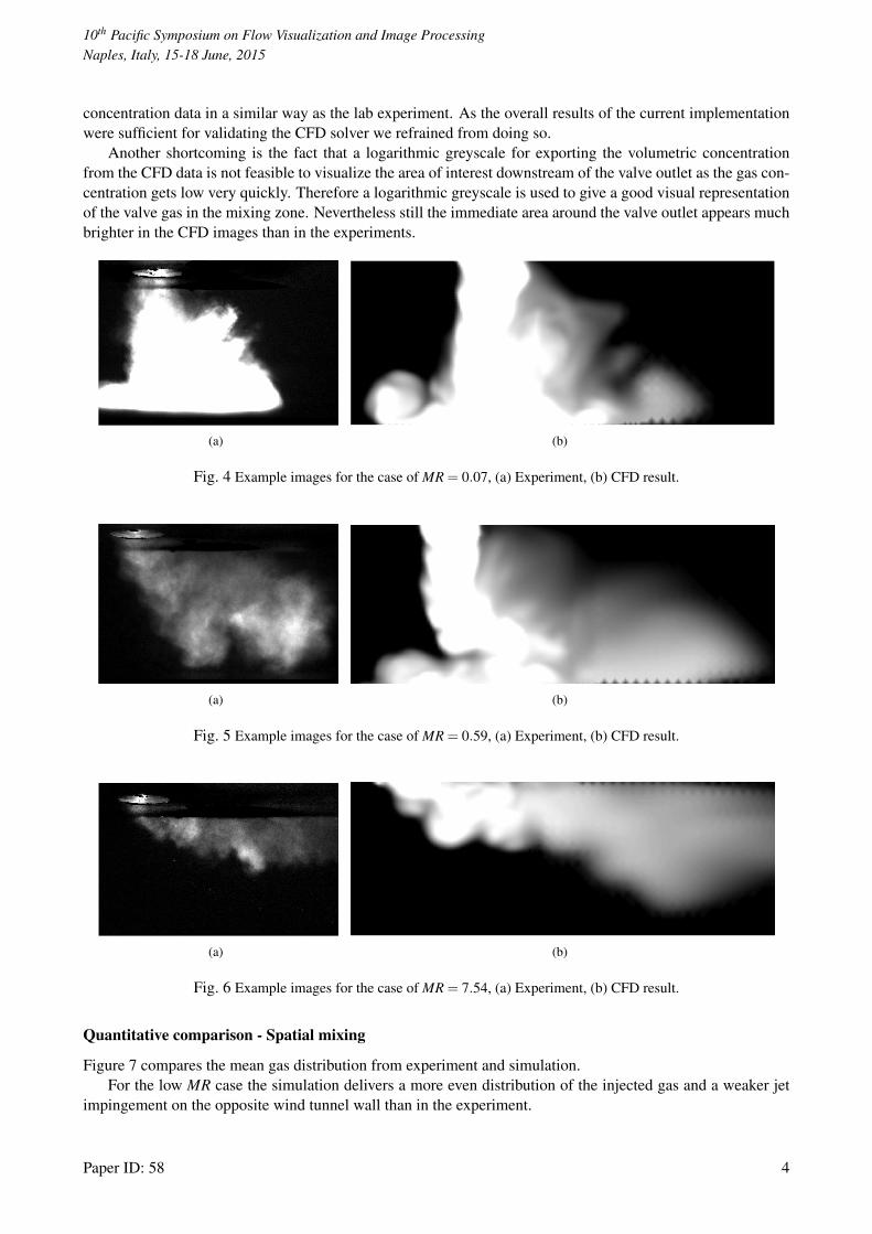
Figures 4, 5 and 6 show a qualitative comparison of single frames from experiments and CFD simulations.As the computational domain is larger than the observable area in the lab setup, the aspect ratio of the givenexamples from experiments and simulations are different.

One can see that the qualitative matching for high and low MR is very good, while for the medium MR casethe jet penetration is a little bit over estimated on the CFD side.

Note that the numerical results only represent the center plane of the CFD domain while the experimentallyobtained images are a perspective view of the three-dimensional problem. For the gas concentration this meansthat the CFD images lack of flow effects in the third direction (depth of the wind tunnel) while the cameraimage can be considered as an integration of the Mie scattering over the channel depth. The method could beimproved by implementing a ray tracing algorithm in the CFD post-processing which allows to integrate the

Paper ID: 58 3

10th Pacific Symposium on Flow Visualization and Image ProcessingNaples, Italy, 15-18 June, 2015

concentration data in a similar way as the lab experiment. As the overall results of the current implementationwere sufficient for validating the CFD solver we refrained from doing so.

Another shortcoming is the fact that a logarithmic greyscale for exporting the volumetric concentrationfrom the CFD data is not feasible to visualize the area of interest downstream of the valve outlet as the gas con-centration gets low very quickly. Therefore a logarithmic greyscale is used to give a good visual representationof the valve gas in the mixing zone. Nevertheless still the immediate area around the valve outlet appears muchbrighter in the CFD images than in the experiments.

(a) (b)

Fig. 4 Example images for the case of MR = 0.07, (a) Experiment, (b) CFD result.

(a) (b)

Fig. 5 Example images for the case of MR = 0.59, (a) Experiment, (b) CFD result.

(a) (b)

Fig. 6 Example images for the case of MR = 7.54, (a) Experiment, (b) CFD result.

Quantitative comparison - Spatial mixing

Figure 7 compares the mean gas distribution from experiment and simulation.For the low MR case the simulation delivers a more even distribution of the injected gas and a weaker jet

impingement on the opposite wind tunnel wall than in the experiment.

Paper ID: 58 4

10th Pacific Symposium on Flow Visualization and Image ProcessingNaples, Italy, 15-18 June, 2015

For the case of medium MR values we observe the opposite situation, that the simulation overestimates thejet penetration as already stated in the previous section.

In the case of high MR numbers the experimental signal gets very weak and noisy because the injected gasis dragged away very quickly in a small area close to the valve outlet. In the simulations the valve gas covers alarger area of the wind tunnel.

In general the agreement is fair. The obvious differences are mainly caused from the problem mentionedbefore, that only 2D CFD data was used and the logarithmic greyscale used to export the CFD data.

(a) (b)

(c)

Fig. 7 Comparison of the mean gas distribution from experiment and simulation for (a) MR = 0.07, (b) MR = 0.59 and(c) MR = 7.54.

Quantitative comparison - Temporal mixing

Figures 8, 9 and 10 show the evolution of the mean and peak values of the luminosity distributions. In the CFDsimulations the gas injection always starts at 10 ms while in the experiments the camera is synchronized to theactuator of the valve. Therefore the signals have different offsets on the time axes.

The threshold to start the time counter was set to 0.2 for the peak signal. To stop the time counter a value of0.15 was used. This small hysteresis eliminates the effect of noisy signals from the experiments. The differenceof the two timestamps gives the mixing time at the selected position. To ensure comparability the same valueswere used for numerical results.

Paper ID: 58 5

10th Pacific Symposium on Flow Visualization and Image ProcessingNaples, Italy, 15-18 June, 2015

Fig. 8 Temporal distribution of injected gas passing the selected line for processing. MR = 0.07.

Fig. 9 Temporal distribution of injected gas passing the selected line for processing. MR = 0.59.

Fig. 10 Temporal distribution of injected gas passing the selected line for processing. MR = 7.54.

Paper ID: 58 6

10th Pacific Symposium on Flow Visualization and Image ProcessingNaples, Italy, 15-18 June, 2015

The resulting mixing times show an excellent agreement of numerical results and experimental data. Table1 gives an overview of the obtained values. Likewise the mean and peak values also show a similar temporalevolution. Even for the noisy signals of the high MR case with larger fluctuations of the mean and peak values(Fig. 10) the matching is very good. This demonstrates the robustness of the method.

MR tmix,Exp (ms) tmix,Sim (ms) deviation0.07 33.6 36.4 3.2%0.59 16.8 17.6 4.7%7.54 13.2 13.2 0%

Table 1 Comparison of mixing times from experiment and CFD.

6 Summary & Outlook

The present study discusses a validation study for a customized CFD solver implemented in OpenFOAM toinvestigate gas mixing efficiency. We introduced a simple image processing method to evaluate spatial andtemporal mixing behaviour and applied this method to experimental as well as numerical results. The overallagreement between CFD results and the lab experiment is very good. This successful validation provides thebasis for further geometry studies of valve mixing devices.

The current method could be further improved by implementing a ray tracing algorithm in the CFD post-processing which would incorporate three-dimensional effects in the exported CFD results.

References

[1] Karagozian, A. R. (2014) The jet in crossflow. Physics of Fluids, vol. 26

[2] Puttinger, S., Holzinger, G., Pirker, S. (2013) Investigation of highly laden particle jet dispersion by theuse of a high-speed camera and parameter-independent image analysis. Powder Technology, vol. 234, pp46-57

Paper ID: 58 7