External geophysics, climate Spatial and temporal variability in maximum, minimum and mean air temperatures at Madhya Pradesh in central India Variabilite ´ spatio-temporelle dans les tempe ´ratures maximales, minimales et moyennes de l’air a ` Madhya Pradesh, Inde centrale Darshana Duhan a, *, Ashish Pandey a , Krishan Pratap Singh Gahalaut b , Rajendra Prasad Pandey c a Department of Water Resources Development and Management, IIT Roorkee, 247667 Roorkee, Uttrakhand, India b Johann Radon Institute for Computational and Applied Mathematics (RICAM), Linz, Austria c National Institute of Hydrology Roorkee, Uttrakhand, India C. R. Geoscience 345 (2013) 3–21 A R T I C L E I N F O Article history: Received 27 June 2012 Accepted after revision 31 October 2012 Available online 19 January 2013 Presented by Michel Petit Keywords: Mann–Kendall test Trend-Free Pre-Whitening Inverse distance weighted interpolation method Mots cle ´s : Test Mann-Kendall Me ´ thode d’interpolation ponde ´re ´e de distance inverse E ´ volution sans pre ´ -blanchiment (TFPW) Madhya Pradesh Inde centrale A B S T R A C T In the present study, an investigation has been made to study the spatial and temporal variability in the maximum, the minimum and the mean air temperatures at Madhya Pradesh (MP), in central India on monthly, annual and seasonal time scale from 1901 to 2002. Further, impact of urbanization and cloud cover on air temperature has been studied. The annual mean, maximum and minimum temperatures are increased by 0.60, 0.60 and 0.62 8C over the past 102 years, respectively. Seasonally, the warming is more pronounced during winter than summer. The temperature decreased during the less urbanized period (from 1901 to 1951) and increased during the more urbanized period (1961 to 2001). It is also found that the minimum temperature increased at higher rate (0.42 8C) followed by the mean (0.36 8C) and the maximum (0.32 8C) temperature during the more urbanized period. Furthermore, cloud cover is significantly negatively related with air temperature in monsoon season and as a whole of the year. ß 2012 Acade ´ mie des sciences. Published by Elsevier Masson SAS. All rights reserved. R E ´ S U M E ´ Dans la pre ´ sente e ´ tude, est recherche ´e la variabilite ´ spatio-temporelle dans les tempe ´ ratures maximales, minimales et moyennes de l’air a ` Madhya Pradesh (MP) en Inde centrale, sur des e ´ chelles de temps mensuelle, annuelle et saisonnie ` re, de 1901 a ` 2012. L’impact de l’urbanisation et de la couverture nuageuse sur la tempe ´ rature de l’air a aussi e ´te ´e ´ tudie ´. Les tempe ´ ratures annuelles moyennes, maximales et minimales ont augmente ´ respectivement de 0,60, 0,60 et 0,62 8C sur les 102 dernie ` res anne ´ es. Si l’on se place du point de vue saisonnier, le re ´ chauffement est plus marque ´ pendant l’hiver que pendant l’e ´te ´. La tempe ´ rature a diminue ´ pendant la pe ´ riode la moins urbanise ´e conside ´re ´e (1901 a ` 1951) et augmente ´ pendant la pe ´ riode la plus urbanise ´e (1961 a ` 2001). Il a aussi e ´te ´ observe ´ que la tempe ´ rature minimale avait augmente ´ d’une valeur plus e ´ leve ´e (0,42 8C), que la tempe ´ rature moyenne (0,36 8C), et la tempe ´ rature maximale (0,32 8C) et ce, durant la pe ´ riode la plus urbanise ´e. En outre, la couverture nuageuse est significativement relie ´e ne ´ gativement a ` la tempe ´ rature de l’air en pe ´ riode de mousson et tout au long de l’anne ´e. ß 2012 Acade ´ mie des sciences. Publie ´ par Elsevier Masson SAS. Tous droits re ´ serve ´s. * Corresponding author. E-mail addresses: [email protected](D. Duhan), [email protected](A. Pandey), [email protected](K.P.S. Gahalaut), [email protected](R.P. Pandey). Contents lists available at SciVerse ScienceDirect Comptes Rendus Geoscience ww w.s cien c edir ec t.c om 1631-0713/$ – see front matter ß 2012 Acade ´ mie des sciences. Published by Elsevier Masson SAS. All rights reserved. http://dx.doi.org/10.1016/j.crte.2012.10.016
Transcript
Ext
Spte
Va
mo
Daa Deb Johc Na
C. R. Geoscience 345 (2013) 3–21
A R
Artic
Rece
Acce
Avai
Pres
Keyw
Man
Tren
Inve
met
Mot
Test
Met
dist
Evol
Mad
Inde
*
rppa
163
http
ernal geophysics, climate
atial and temporal variability in maximum, minimum and mean airmperatures at Madhya Pradesh in central India
riabilite spatio-temporelle dans les temperatures maximales, minimales et
yennes de l’air a Madhya Pradesh, Inde centrale
rshana Duhan a,*, Ashish Pandey a, Krishan Pratap Singh Gahalaut b, Rajendra Prasad Pandey c
partment of Water Resources Development and Management, IIT Roorkee, 247667 Roorkee, Uttrakhand, India
ann Radon Institute for Computational and Applied Mathematics (RICAM), Linz, Austria
tional Institute of Hydrology Roorkee, Uttrakhand, India
T I C L E I N F O
le history:
ived 27 June 2012
pted after revision 31 October 2012
lable online 19 January 2013
ented by Michel Petit
ords:
n–Kendall test
d-Free Pre-Whitening
rse distance weighted interpolation
hod
s cles :
Mann-Kendall
hode d’interpolation ponderee de
ance inverse
ution sans pre-blanchiment (TFPW)
hya Pradesh
centrale
A B S T R A C T
In the present study, an investigation has been made to study the spatial and temporal
variability in the maximum, the minimum and the mean air temperatures at Madhya
Pradesh (MP), in central India on monthly, annual and seasonal time scale from 1901 to
2002. Further, impact of urbanization and cloud cover on air temperature has been
studied. The annual mean, maximum and minimum temperatures are increased by 0.60,
0.60 and 0.62 8C over the past 102 years, respectively. Seasonally, the warming is more
pronounced during winter than summer. The temperature decreased during the less
urbanized period (from 1901 to 1951) and increased during the more urbanized period
(1961 to 2001). It is also found that the minimum temperature increased at higher rate
(0.42 8C) followed by the mean (0.36 8C) and the maximum (0.32 8C) temperature during
the more urbanized period. Furthermore, cloud cover is significantly negatively related
with air temperature in monsoon season and as a whole of the year.
� 2012 Academie des sciences. Published by Elsevier Masson SAS. All rights reserved.
R E S U M E
Dans la presente etude, est recherchee la variabilite spatio-temporelle dans les temperatures
maximales, minimales et moyennes de l’air a Madhya Pradesh (MP) en Inde centrale, sur des
echelles de temps mensuelle, annuelle et saisonniere, de 1901 a 2012. L’impact de
l’urbanisation et de la couverture nuageuse sur la temperature de l’air a aussi ete etudie. Les
temperatures annuelles moyennes, maximales et minimales ont augmente respectivement
de 0,60, 0,60 et 0,62 8C sur les 102 dernieres annees. Si l’on se place du point de vue saisonnier,
le rechauffement est plus marque pendant l’hiver que pendant l’ete. La temperature a
diminue pendant la periode la moins urbanisee consideree (1901 a 1951) et augmente
pendant la periode la plus urbanisee (1961 a 2001). Il a aussi ete observe que la temperature
minimale avait augmente d’une valeur plus elevee (0,42 8C), que la temperature moyenne
(0,36 8C), et la temperature maximale (0,32 8C) et ce, durant la periode la plus urbanisee. En
outre, la couverture nuageuse est significativement reliee negativement a la temperature de
l’air en periode de mousson et tout au long de l’annee.
� 2012 Academie des sciences. Publie par Elsevier Masson SAS. Tous droits reserves.
D. Duhan et al. / C. R. Geoscience 345 (2013) 3–214
1. Introduction
Temperature is the second most important meteoro-logical variable after precipitation because it can be relatedto solar radiation and thus with both evaporation andtranspiration processes which constitute an importantphase of the hydrologic cycle. IPCC (2007) reported theincreasing tendencies in temperature in many areas of theworld in space and time. Nicholls and Collins (2006) foundthat the average maximum temperature in Australia hasincreased by 0.6 8C from 1910 to 2004 and minimumtemperature by 1.2 8C from 1950 to 2004. The increasingtrend in monthly and seasonal surface temperature inEurope is warmer in late 20th and early 21st century thanthat of any time during the past 500 years (Luterbacheret al., 2004). In North America, annual mean air tempera-ture is increased during the period of 1955 to 2005, withthe greatest warming in Alaska and northwestern Canada.For Canada as a whole, the annual mean temperature hasincreased by 1.2 8C over the past 53 years (Vincent et al.,2007).
In Asia, increasing trends have been observed across theseven sub regions of Asia (IPCC, 2007). The observed rise inmean annual temperature is 2 to 3 8C in Russia (Petersonet al., 2002; Savelieva et al., 2000), 1.8 8C in Mongolia(Batima et al., 2005), 0.7 8C in Northwest China (Shi et al.,2002), 1.0 8C in Japan (Ichikawa, 2004), 0.23 8C in Korea(Jung et al., 2002) and 0.14 8C in Philippines (Cruz et al.,2006).
In India also increasing trend is found in the annualmean temperature, annual maximum temperature andannual minimum temperature (Arora et al., 2005; Dashet al., 2007; Kothawale and Rupa Kumar, 2005; Pant andKumar, 1997; Sinha Ray and De, 2003). Few researchstudies have been conducted separately on various cities inIndia (Dhorde et al., 2009; Gadgil and Dhorde, 2005) andfound the mix trends in temperature series.
Research studies carried out by various researchersfound that the increasing trends in air temperature havebeen related to several factors such as increased concen-trations of anthropogenic greenhouse gases (De andMukhopadhyay, 1998; Easterling et al., 1997; Qianget al., 2004; Soltani and Soltani, 2008), increased emissionsof anthropogenic aerosols (Cohen and Stahill, 1996;Ramanathan et al., 2007), increased cloud cover andurbanization (Ji and Zhou, 2011; Tabari and HosseinzadehTalaee, 2011). Further, IPCC (2007) reported that most ofthe observed increase in average temperature since themid-twentieth century is very likely due to the observedincrease in anthropogenic greenhouse gas concentrations.The major greenhouse gases (GHGs) are water vapor,which causes about 36–70% of the greenhouse effect;carbon dioxide (CO2), which causes 9–26%; methane (CH4),which causes 4–9%; and ozone (O3), which causes 3–7%(Kiehl and Trenberth, 1997). GHGs warm the surface andthe atmosphere with significant implications for rainfallretreat of glaciers and sea ice, sea level, among otherfactors (Ramanathan and Feng, 2009). The greenhouseeffect is the phenomenon where water vapour, CO2, CH4
and other atmospheric gases absorb outgoing infrared
absorb and emit long wave radiation, while aerosolsabsorb and scatter solar radiation (Ramanathan and Feng,2009).
Ozone is a secondary air pollutant that is formed by thetransformation reactions of primary air pollutants, espe-cially nitrogen dioxide (NO2). O3 is one of the majorpollutants in the atmosphere, causing several damages onhuman health, climate, vegetation and materials (Fuhreret al., 1997; Karnosky et al., 2005; Musselman andMassman, 1999; Ollerenshaw et al., 1999; Smidt andHerman, 2004). Ozone concentration builds up in theatmosphere from several natural and anthropogenicsources. These include:
� downward transport of stratospheric O3 through the freetroposphere to near-ground level;� in situ O3 production from methane emitted from
swamps and wetlands reacting with natural nitrogenoxides (NOx);� production of O3 from reaction of volatile organic
compounds (VOCs) with NOx;� long-range transport of O3 from distant pollution sources
(EPA, 1993; Kondratyev and Varotsos, 2001a, 2001b;Varotsos et al., 2004).
There are several studies reporting the increase of thesurface O3 (Bojkov, 1986; Cartalis and Varotsos, 1994; Jaffeet al., 2003; Lee et al., 1998; Lisac and Grubisic, 1991; Nolleet al., 2005; Oltmans et al., 1998; Vingarzan, 2004;Vingarzan and Thomson, 2004). Comparisons of ozonebackground levels with those measured in the late 19th–early 20th centuries indicate that current ozone levels haverisen by approximately two times (Bozo and Weidinger,1995; Cartalis and Varotsos, 1994; Staehelin et al., 1994).The main factors for high ozone level episodes are theincrease of temperature, photolysis reactions of nitrogenoxides and the variation in boundary layer as function oftemperature during the day and the night times (Pireset al., 2012).
Under a warmer climate, the arid and semiarid regionlike MP could experience severe water stress due to thedecline in soil moisture. Agriculture is the mainstay of theState’s economy as it provides 71% of employment. Sincethe agricultural productivity is likely to suffer severely dueto higher temperatures and no study was found inliterature on spatial and temporal variability of tempera-ture at Madhya Pradesh (MP), the aims of this study are:
� to investigate the spatial and temporal variability oftemperature of this region;� to examine the relationship of cloud cover with
temperature variables;� to find the impact of urbanization on temperature.
2. Method and material
2.1. Details of study area
The State of MP is centrally located and is often called
the ‘‘Heart of India’’, comprising a geographical area of radiation, resulting in the raising of the temperature. GHGs
D. Duhan et al. / C. R. Geoscience 345 (2013) 3–21 5
,000 km2, occupying 14.5% of the area of India. Thete is bordered by seven other States: Uttar Pradesh,ar, Orissa, Andhra Pradesh, Maharashtra, Gujarat andasthan. The study area extends from 218170 N to360 N and 748020 N to 828260 E covering 45 districts.
has a subtropical climate. There are three distinctsons: summer (March to May), winter (November toruary), and the intervening rainy months of thethwest monsoon (June to October). MP experiencesreme temperatures both during summer and winter.summer, the temperature goes up to 42 8C, and inter it falls tremendously to 10 8C. The temperature
rts rising from March and it starts falling fromober. The temperature also varies from place toce in the State. The hottest place is Bhind in summerere the temperature reaches up to 45 8C, while inpal the temperature is closer to 43 8C. The averageperature in winter is around 10 8C. Rainfall increases
west to east and decreases towards north. The Stateeives maximum rainfall from June to September.ual average rainfall varied from 694.42 mm in
thwest (Westnimar station) part of the MP to about7.28 mm in eastern part (Mandla station) (Darshana
Pandey, 2013) of MP. The latitudinal decline infall and longitudinal increase decide the cropping
tems that are grown across the State. The croppingterns in MP change with rainfall; for example, thetern part of the State is characterized by its rice basedpping systems and the central and western parts of State have soybean based cropping systems whereses and oilseed occupy an important place. The State
been delineated into five major crop zones, namely:; rice-wheat; wheat; jowar-wheat; cotton-jowar andbean.
2.2. Data description
Monthly maximum, minimum and mean air tempera-ture and cloud cover (%) data of 45 stations covering a periodof 102 years (1901 to 2002) were downloaded from theIndian Meteorological Department (IMD) site India waterportal (http://www.indiawaterportal.org/metdata). Popula-tion data was collected from the Census of India (2011)publication. Fig. 1 shows the locations of meteorologicalstations. Data quality control is a necessary step; however,since Mann–Kendall (MK) test is a rank-based nonparamet-ric test, they are robust against outliers. On the other hand,outliers play a key role in parametric tests and in assessingthe magnitude of the possible changes by computing means(moments) and linear regression (Darshana and Pandey,2013). For the present study the data series were plotted todetect the outliers. After visual detection of outliers, thesuspected values were calculated using the normal ratiomethod. As all series were complete, no gap filling methodwas needed. November, December, January and Februarywere considered for the analysis of winter temperature asthese 4 months record the lowest temperatures. Whilecomputing the mean for winter season, December of theprevious year was included. March, April and May are themonths with highest mean maximum temperatures and,therefore, represent the summer season. June to Octoberconstitute monsoon season. The monthly data were aver-aged to provide annual and seasonal values for each year.
2.3. Methodology
2.3.1. Trend detection
The moving average or running mean is a conventionalprocedure used to reduce the inter-annual variability of
1. Location of the meteorological stations at Madhya Pradesh.
1. Localisation des stations meteorologiques de Madhya Pradesh (MP).
D. Duhan et al. / C. R. Geoscience 345 (2013) 3–216
time series (Sneyers, 1992). A 10-year running average wasused in the present study. Linear trend represented by theslope of the simple least square regression line providedthe rate of rise/fall in the variable. Using the value of therate of change, the total change over the last 102 years wascomputed.
Autocorrelation is also called lagged correlation or serialcorrelation which refers to the correlation of a time serieswith its own past and future values (Madnani, 2009). In theterminology of the atmospheric sciences, this dependencethrough time is usually known as persistence (Chattopad-hyay et al., 2011). Persistence can be defined as the existenceof (positive) statistical dependence among successive valuesof the same variable, or among successive occurrences of agiven event (Wilks, 2006). The short-range correlations aredescribed by the autocorrelation function, which declinesexponentially with a certain decay time. However, for thelong-range correlations, the autocorrelation functiondeclines as a power-law (Varotsos, 2005b). The directcalculation of the autocorrelation function is usually notappropriate to distinguish among different decay patterns atlong lags, due to noise superimposed on the data (Galmariniet al., 2004; Kantelhardt et al., 2002; Stanley, 1999). Thedetrended fluctuation analysis (DFA), introduced by Penget al. (1994), is a well-established method for determiningthe scaling behavior of noisy data in the presence of trendswithout knowing their origin and shape (Talkner andWeber, 2000). Therefore, the DFA method was used in thepresent study to check the scaling behavior of monthly airtemperatures variable namely maximum, minimum andmean air temperature data over MP.
Nonparametric tests are also referred to as distribution-free tests. These tests have the several advantages overparametric methods. Some of these advantages include:
� they do not require the assumption of normality or theassumption of homogeneity of variance;� they compare medians rather than means and, as a
result, if the data have one or two outliers, their influenceis negated;� prior transformations are not required, even when
approximate normality could be achieved;
� greater power is achieved for the skewed distributions;� data below the detection limit can be incorporated
without fabrication of values or bias (Helsel, 1987).
The influence of serial correlation in the time series onthe results of MK test (Kendall, 1975; Mann, 1945) hasbeen discussed in the literature (Yue et al., 2002). Hence tosolve the issue of autocorrelation, the Trend-Free Pre-Whitening (TFPW)-MK procedure proposed by Yue et al.(2002) was used. Lag-1 autocorrelation coefficient (Haan,2002) was used to detect the presence of serial correlationin data series. The temperature series which were foundserially independent, MK test was directly applied to theoriginal sample data. However, the series which werefound serially correlated, pre-whitening was used beforeapplying the MK test. Confidence levels of 90% and 95%and 99% were taken as thresholds to classify thesignificance of positive and negative temperature trends.The brief explanations of methods used are given in theAppendix.
To explore the spatial distribution of trends fortemperature variables, the Sen Slope estimator (b)proposed by Sen (1968) was interpolated using ArcGIS9.3 based on each individual station b value.
2.3.2. Effect of urbanization on temperature
To study the effect of urbanization on temperature, thestudy period is categorized into two parts; less urbanizedperiod (LUP) and more urbanized period (MUP). The LUPand MUP are identified based on the population trends.Fig. 2 shows that up to 1951 population growth was slow,but after 1951 population growth was fast as compared to1951. Considering this variation in the growth pattern, theperiod from 1901 to 1951 is identified as LUP and theperiod from 1961 to 2001 is characterized by MUP.
2.3.3. The relationship of air temperature and cloud cover
The Pearson correlation test is applied to detect therelationship between cloud cover and temperature vari-ables on annual and seasonal basis. The significance ofcorrelation is tested at a 5% significance level usingKendall-tau method.
Fig. 2. Less urbanized period (LUP) and more urbanized period (MUP) at Madhya Pradesh.
Fig. 2. Periode de moindre urbanisation (LUP) et d’urbanisation plus prononcee (MUP) a Madhya Pradesh.
3. R
3.1.
skeannstatfrom0.5methepostheandKurof ato
mearoinvannfromaveconaretem
3.2.
tem
recsaidtem200TalKirran190ser
Fig.
min
Fig.
Mad
D. Duhan et al. / C. R. Geoscience 345 (2013) 3–21 7
esults and discussion
Preliminary analysis
The statistical parameters (mean, standard deviation,wness, kurtosis and coefficient of variation) of theual mean temperature have been computed for eachion. The annual mean temperature in the State varied
24.34 to 26.61 8C and standard deviation from 0.37 to0 during the 102 years. The skewness, which is aasure of asymmetry in a frequency distribution around
mean, varied from �0.39 to 0.27, predominantlyitive skewness, with an average around 0.02 indicating
annual temperature during the period is asymmetric it lies to the right of the mean over all the stations.tosis, a statistic parameter describing the peakedness
symmetrical frequency distribution, varied from �0.570.55. The coefficient of variation (CV), a statisticalasure of the dispersion of data points in a data seriesund the mean, was computed for all stations in order toestigate the spatial pattern of inter-annual variability ofual temperature over the study area. The CV varied
1.45% (Balaghat district) to 1.99% (Katni district). Therage CV of entire MP was 1.6 percent. It can becluded that the zones of usually higher temperatures
the zones of least variability, and the zones of lowestperatures are the zone of highest variability.
Analysis of autocorrelation structure of the monthly air
perature
Koscielny-Bunde et al. (1998) stated that temperatureords follow a universal scaling law. This behavior was
to be found in numerous daily and monthlyperature data sets (Eichner et al., 2003; Kiraly et al.,6; Koscielny-Bunde et al., 1998; Maraun et al., 2004;
kner and Weber, 2000; Tsonis et al., 2000; Varotsos andk-Davidoff, 2006). In order to test the short and long-ge correlation in the monthly temperature series from1 to 2002 (n = 1224) at MP, DFA1 was used. The time
ies is first integrated using Eq. (1) (Appendix) to
exaggerate the non-stationarity of the original data, reducethe noise level, and generate a time series corresponding tothe construction of a random walk that has the values ofthe original time series as increments. After that theintegrated time series is divided into boxes of equal lengthd. In each box of length d, a least squares line (orpolynomial curve of order 1) is fitted to the data(representing the trend in that box). Further, the integratedtime series is detrended using Eq. (2) (Appendix) bysubtracting the local trend in each box. The root-mean-square fluctuation of this integrated and detrended timeseries is calculated and denoted as F(d). This computationis repeated over all time scales (box sizes), from allminimum box size to maximum box size, to characterizethe relationship between F(n), the average fluctuation, andn, the box size. The minimum box size used is 2k + 2 (wherek is the order of polynomial curve, in this case K = 1) and themaximum box size used is one-tenth of the length of theinput series (Ivanov et al., 2001). A log-log plot of the root-mean-square fluctuation function Fd and Dt of theintegrated and detrended monthly air temperature seriesover MP is shown in Fig. 3. Exponents (slope of log-log plot)a of 1.21 (� 0.07), 1.14 (� 0.09) and 1.19 (� 0.08) were foundfor maximum, minimum and mean air temperature respec-tively, which indicates that long-range power-law correla-tions prevail in temperature data over MP. It can beconcluded that air temperature over the MP exhibitspersistent long-range correlations.
3.3. Analysis of temperature anomalies
The temperature anomalies have been computed forbetter understanding of the observed trends in theminimum temperature, the maximum temperature andthe mean temperature during the time period of 102 years(1901 to 2002). Figs. 4–6 show the annual temperatureanomalies in the maximum, minimum and mean temper-ature averaged over the MP. A well-marked warming trendis observed in the maximum temperature (Fig. 4). FromFig. 4, it was observed that the anomaly became positiveafter 1947 and the positive enhancement became sharp till
3. Log-log plot of root-mean-square fluctuation function (F(d)) versus temporal change Dt (in months) over MP for maximum air temperature (a) for
imum air temperature (b) and for mean air temperature (c).
3. Diagramme log-log de la fonction (F(d)) de fluctuation de la valeur quadratique moyenne en fonction du changement temporel Dt (en mois) sur
hya Pradesh pour les temperatures de l’air maximale (a), minimale (b) et moyenne (c).
D. Duhan et al. / C. R. Geoscience 345 (2013) 3–218
year 2002. The linear trend line indicates that themaximum temperature is increased by 0.60 8C in the last102 years over MP. Further, the minimum temperature(Fig. 5) also shows the positive anomalies after 1947. Theincrease in minimum temperature was 0.62 8C during the102 years. Furthermore, the annual mean temperatureshowed an increase of 0.60 8C (Fig. 6) over the MP. From theabove, it reveals that the night temperature is increasing atfaster rate than day temperature.
3.4. Decadal variations of annual and seasonal temperature
To ascertain whether the warming rate was uniformthroughout the last century or not, decade-to-decade rates
over entire MP were computed. The decadal variation oftemperature was studied for the annual and seasonal basis(Table 1) and compared with long-term series (1901 to2002). In general, for all the temperature variables, episodicvariation was noticed and up to 1960s, there is a coolerperiod of decreasing temperature (Table 1). This period wasfollowed by a warming period. Real warming appears tohavestartedinthe decadeof1961to1970withamodest rateand continued till the end of the century. The warming rateappears to be highest during the period from 1971 to 1980 ascompared to the other periods. The warming rates are lessafterwards, as compared to 1980 in the rest of the decades.
The mean minimum temperature anomaly was nega-tive from 1901–1910 to 1951–1960. However, it becomes
Fig. 6. Anomalies in annual mean temperature at Madhya Pradesh from 1901 to 2002.
Fig. 6. Anomalies dans la temperature moyenne annuelle a Madhya Pradesh, sur la periode 1901 a 2002.
pos0.8of lanodec197highigFuranodecThemoto 1wa
posin 1ano194of t(1.3anawinvallonshoto 1shoma
3.5.
ove
thetemtrentestpresignminmu
Tab
Dec
Tabl
Vari
De
19
19
19
19
19
19
19
19
19
19
19
Tmax
D. Duhan et al. / C. R. Geoscience 345 (2013) 3–21 9
itive from 1961 to 1970. The highest anomaly was3 8C in 1971 to 1980, which was higher than the anomalyong-term mean (1901 to 2002). The winter temperaturemaly was negative from 1911–1920 to 1941–1950ade and positive in 1901 to 1910, 1951 to 1960, 1961 to0, 1971 to 1980, 1981 to 1990 and 1991 to 2002. The
hest anomaly was 1.93 8C during 1971 to 1980, which isher than the long-term annual series (1901 to 2002).ther, in summer, the temperature shows a positivemaly in the 1961 to 1970, 1981 to 1990 and 1991 to 2002ades, and a negative anomaly during rest of the decades.
inter decadal variation of temperature anomaly in thensoon season was positive during the 1921 to 1930, 1961970 and 1971 to 1980 decades, out of which the highest
s 0.68 8C in the 1971 to 1980 decade.The annual maximum temperature anomaly wasitive after the decade 1951 to 1960, and the highest961 to 1970 decade (0.84 8C). The winter temperaturemaly was negative in four decades i.e. 1911–1920 to1–1950. However, positive anomaly was found in rest
he decades and highest in the decade from 1961 to 19707 8C) than the long-term average annual over thelysis period. The summer anomaly was lower than theter anomaly in all the decades, and had its highest
ue of 0.82 8C during 1981 to 1990 in comparison to theg-term analysis period. In monsoon, the temperaturews the positive anomaly only in the periods from 1921930 and 1961 to 1970. The mean temperature anomalyws the same decadal pattern like minimum andximum temperatures on the annual and seasonal scales.
Results of Mann–Kendall test and linear regression test
r entire Madhya Pradesh
MK test and linear regression test were used to evaluate monthly, annual and seasonal long-term changes in airperature over entire MP. Apart from this, the lineard fitted to the data was also tested with the Student t-
to verify results obtained by the MK test and results aresented in Table 2. The results of the MK test reveal theificant increasing trend in almost all months ofimum, maximum and mean temperature. The mini-
m temperature showed the significant warming trend
in February, March, April, October, November and Decem-ber during the analysis period from 1901 to 2002. Usingthe linear regression test, the month wise rate of change ofminimum temperature varied from �0.47 8C (June) to1.94 8C (November). The significant increasing trend wasobserved in annual, winter and summer temperatures. It isfound from seasonal analysis that the winter minimumtemperature showed the maximum increasing rate(1.24 8C) followed by summer (0.61 8C) and monsoon(0.08 8C) season.
Using the MK test, the maximum temperature showedthe significant warming trend in February, March, October,November and December at 5% significance level. Usinglinear trend the monthly rate of change of the maximumtemperature varied from �0.41 (June) to 1.76 (Novem-ber) 8C/102 years. The results reveal the significantincrease in annual, winter and summer maximumtemperatures. The increase in annual maximum tempera-ture was 0.60 8C from 1901 to 2002 over the MP.Seasonally, the winter temperature has the maximumincrease (1.21 8C) followed by summer (0.59 8C) andmonsoon (0.07 8C) season.
Further, month wise rate of change of mean tempera-ture varied from �0.36 8C (June) to 1.96 8C (November).The increase in annual mean temperature was 0.60 8Cduring the analysis period of 1901 to 2002 over the MP.Seasonal analysis shows that the winter mean temperaturehas the maximum increasing rate (1.20 8C) followed bysummer (0.59 8C) and monsoon (0.07 8C) season. The aboveresults suggest that the climate of the MP is gettingwarmer and warming is more pronounced during nightthan during day.
3.6. Stations wise trend in annual and seasonal temperature
variables
Table 3 shows the results of MK test. The annualmaximum, minimum and mean temperature showed astatistically significant increasing trend over all thestations. The seasonal maximum temperature showed astatistically significant increasing trend at all the stations(at 5% significance level) in the winter season, 25 stations(at 5% significant level) in the summer season and eight
le 1
adal variation of temperature variables over Madhya Pradesh.
eau 1
ation decennale des variables de temperature sur Madhya Pradesh.
: maximum temperature; Tmin: minimum temperature; Tmean: mean temperature range; A: annual; W: winter; S: summer; M: monsoon.
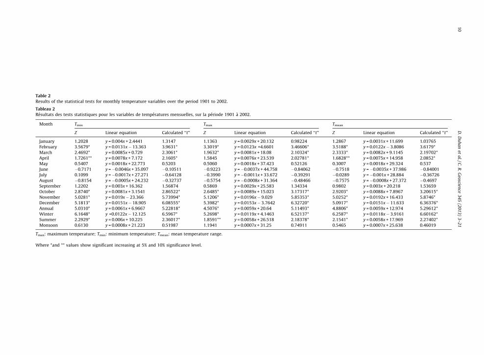
Table 2
Results of the statistical tests for monthly temperature variables over the period 1901 to 2002.
Tableau 2
Resultats des tests statistiques pour les variables de temperatures mensuelles, sur la periode 1901 a 2002.
Month Tmin Tmax Tmean
Z Linear equation Calculated ‘‘t’’ Z Linear equation Calculated ‘‘t’’ Z Linear equation Calculated ‘‘t’’
January 1.2028 y = 0.004x + 2.4441 1.3147 1.1363 y = 0.0029x + 20.132 0.98224 1.2867 y = 0.0031x + 11.699 1.03765
February 3.5679* y = 0.0131x� 13.363 3.9631* 3.3019* y = 0.0123x +4.6601 3.46606* 3.5188* y = 0.0122x� 3.8086 3.6179*
March 2.4692* y = 0.0085x + 0.729 2.3061* 1.9632* y = 0.0081x + 18.08 2.10324* 2.3333* y = 0.0082x + 9.1145 2.19702*
April 1.7261** y = 0.0078x + 7.172 2.1605* 1.5845 y = 0.0076x + 23.539 2.02781* 1.6828** y = 0.0075x + 14.958 2.0852*
May 0.5407 y = 0.0018x + 22.773 0.5203 0.5060 y = 0.0018x + 37.423 0.52126 0.3007 y = 0.0018x + 29.324 0.537
June �0.7171 y =�0.0046x + 35.097 �0.10511 �0.9223 y =�0.0037x + 44.758 �0.84062 �0.7518 y =�0.0035x + 37.986 �0.84001
July 0.1099 y =�0.0017x + 27.271 �0.64128 �0.3990 y =�0.0011x + 33.672 �0.39291 �0.0289 y =�0.001x + 28.884 �0.36726
August �0.8154 y =�0.0005x + 24.232 �0.32737 �0.5754 y =�0.0008x + 31.364 �0.48466 �0.7575 y =�0.0008x + 27.372 �0.4697
September 1.2202 y = 0.003x + 16.362 1.56874 0.5869 y = 0.0029x + 25.583 1.34334 0.9802 y = 0.003x + 20.218 1.53659
October 2.8740* y = 0.0081x + 3.1541 2.86522* 2.6485* y = 0.0089x + 15.023 3.17317* 2.9203* y = 0.0088x + 7.8967 3.20615*
November 5.0281* y = 0.019x� 23.366 5.73994* 5.1206* y = 0.0196x� 9.029 5.85353* 5.0252* y = 0.0192x + 16.433 5.8746*
December 5.1813* y = 0.0151x� 18.905 6.08555* 5.3982* y = 0.0153x� 3.7642 6.32720* 5.0917* y = 0.0151x� 11.633 6.36376*
Annual 5.0310* y = 0.0061x + 6.9667 5.22818* 4.5076* y = 0.0059x + 20.64 5.11493* 4.8806* y = 0.0059x + 12.974 5.29612*
Winter 6.1648* y =0.0122x� 12.125 6.5967* 5.2698* y = 0.0119x + 4.1463 6.52137* 6.2587* y = 0.0118x� 3.9161 6.60162*
Summer 2.2929* y = 0.006x + 10.225 2.36017* 1.8591** y = 0.0058x + 26.518 2.18378* 2.1541* y = 0.0058x + 17.969 2.27402*
Monsoon 0.6130 y = 0.0008x + 21.223 0.51987 1.1941 y = 0.0007x + 31.25 0.74911 0.5465 y = 0.0007x + 25.638 0.46019
Tmax: maximum temperature; Tmin: minimum temperature; Tmean: mean temperature range.
Where *and ** values show significant increasing at 5% and 10% significance level.
D.
Du
ha
n et
al.
/ C
. R
. G
eoscien
ce 3
45
(20
13
) 3
–2
11
0
statstatresthestat27
statHowtrenstatstatthe(inc
Tab
Resu
Tabl
Resu
Na
Ba
Ba
Be
Bh
Bh
Ch
Ch
Da
Da
De
Dh
Di
Ea
Gu
Gw
Ha
Ho
In
Ja
Jh
Ka
M
M
M
Na
Ne
Pa
Ra
Ra
Ra
Re
Sa
Sa
Se
Se
sh
Sh
Sh
Sh
Sid
Ti
Uj
Um
Vi
W
Tmax
Whe
D. Duhan et al. / C. R. Geoscience 345 (2013) 3–21 11
ions (five stations at 5% significance level and threeions at 10% significance level) in the monsoon season,
pectively. The seasonal minimum temperature reveal statistically significant increasing trend at all theions in the winter season (at 5% significance level) andstations (19 stations at 5% significance level and eightions at 10% significance level) in the summer seasons.ever, in the monsoon season, it shows the increasing
d in only five stations and the decreasing trend in threeions. Further, the seasonal mean temperature showed aistically significant trend at 5% significance level at all
stations (increasing) in winter season, 27 stationsreasing) in summer and nine stations (six increasing
and three decreasing) in the monsoon season. It isobserved that in some stations there is a significant trendat the annual scale but there is a no significant trend at theseasonal scale.
3.7. Spatial distribution of temporal change in temperature
Exploring long-term changes in temperature patterns isone of the important components in climate changeanalysis. Using spatial analysis more insight into localand regional trends of climate pattern can be provided forbetter understanding of climate (Boyles and Raman, 2003).In this study, b was used instead of the least squares
le 3
lts of Mann–Kendall test in temperature series over the Madhya Pradesh.
eau 3
ltats du test Mann–Kendall dans les series de temperatures sur Madhya Pradesh.
: maximum temperature; Tmin: minimum temperature; Tmean: mean temperature range; A: annual; W: winter; S: summer; M: monsoon.
re ▲ and ▲ ▲: significant increasing at 5% & 10%, ▲and ▲ ▲: significant decreasing at 5% & 10%, + & �: non-significant increasing & decreasing trend.
D. Duhan et al. / C. R. Geoscience 345 (2013) 3–2112
estimate because it is less sensitive to the non-normality ofthe distribution and less affected by extreme values oroutliers in the series (Zhang et al., 2000). An inversedistance weighted interpolation method (IDW), which isbased on the assumption that the interpolation surfaceshould be influenced most by nearby points and less bymore distant points (Gemmer et al., 2004) was used. Avariable search radius with a minimum sample of 12 pointswas used. To control the significance of the surroundingpoint on the interpolated value the exponent of distance(power) four was used because the higher power results inless influence from distant points. The spatial distributionsof the temperature variable on annual and seasonal basesare shown in Figs. 7–18.
3.7.1. Maximum temperature trend
Fig. 7 showed the spatial distribution pattern oftemporal change in the annual maximum temperature.The increase in magnitude of the annual maximum
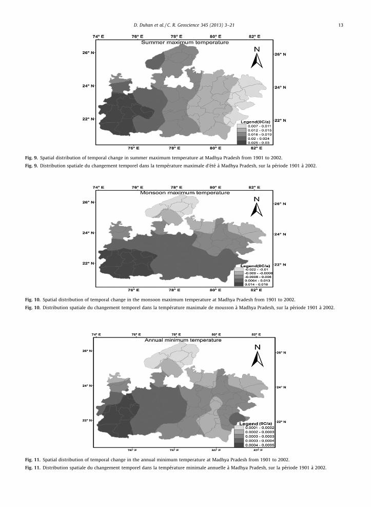
temperature varied from 0.0001 to 0.007 8C/year in mostpart of MP but it exceeded 0.007 8C/year in some areas,such as Seoni and Chindwara. The presence of bump nearthe border may be due to the interpolation that has beenperformed using observations inside the Madhya Pradesh.Fig. 8 shows the spatial distribution of winter maximumtemperature whose magnitude varied from 0.0002 to0.005 8C/year in most part of MP but it exceeded 0.005 8C/year in some areas, such as Balaghat station. Again thepresence of bump near the border may be due to theinterpolation that has been performed using observationsinside the Madhya Pradesh. Furthermore, the magnitude ofthe summer maximum temperature (Fig. 9) varied from0.007 to 0.03 8C/year from east to west MP. Fig. 10 showsthe spatial distribution of monsoon maximum tempera-ture. Some parts of MP show the cooling trend and somepart shows the warming trend. The cooling trend has beenobserved in southwestern MP, which varied from �0.02 to�0.0001 8C/year and the remaining part of MP showed the
Fig. 7. Spatial distribution of temporal change in annual maximum temperature at MP from 1901 to 2002.
Fig. 7. Distribution spatiale du changement temporel dans la temperature maximale annuelle a Madhya Pradesh, sur la periode 1901 a 2002.
Fig. 8. Spatial distribution of temporal change in winter maximum temperature at Madhya Pradesh from 1901 to 2002.
Fig. 8. Distribution spatiale du changement temporel dans la temperature maximale d’hiver a Madhya Pradesh, sur la periode 1901 a 2002.
Fig. 9. Spatial distribution of temporal change in summer maximum temperature at Madhya Pradesh from 1901 to 2002.
Fig. 9. Distribution spatiale du changement temporel dans la temperature maximale d’ete a Madhya Pradesh, sur la periode 1901 a 2002.
Fig. 10. Spatial distribution of temporal change in the monsoon maximum temperature at Madhya Pradesh from 1901 to 2002.
Fig. 10. Distribution spatiale du changement temporel dans la temperature maximale de mousson a Madhya Pradesh, sur la periode 1901 a 2002.
Fig. 11. Spatial distribution of temporal change in the annual minimum temperature at Madhya Pradesh from 1901 to 2002.
Fig. 11. Distribution spatiale du changement temporel dans la temperature minimale annuelle a Madhya Pradesh, sur la periode 1901 a 2002.
D. Duhan et al. / C. R. Geoscience 345 (2013) 3–21 13
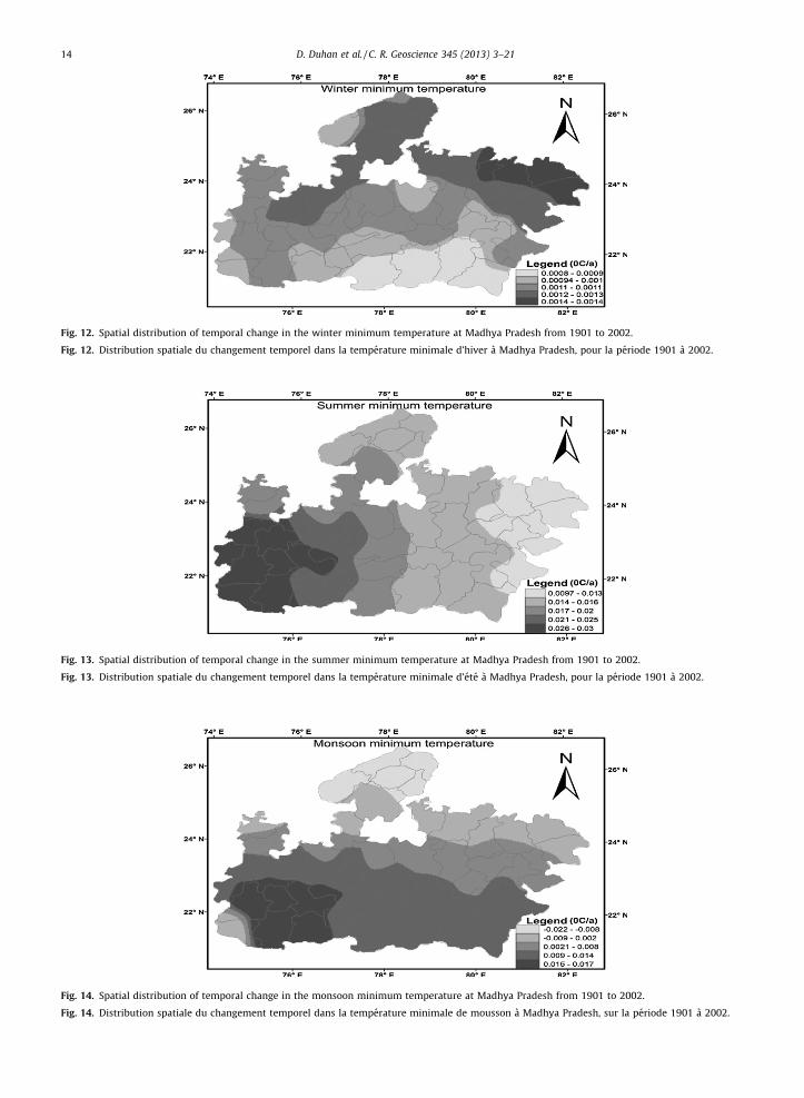
Fig. 12. Spatial distribution of temporal change in the winter minimum temperature at Madhya Pradesh from 1901 to 2002.
Fig. 12. Distribution spatiale du changement temporel dans la temperature minimale d’hiver a Madhya Pradesh, pour la periode 1901 a 2002.
Fig. 14. Spatial distribution of temporal change in the monsoon minimum temperature at Madhya Pradesh from 1901 to 2002.
Fig. 14. Distribution spatiale du changement temporel dans la temperature minimale de mousson a Madhya Pradesh, sur la periode 1901 a 2002.
Fig. 13. Spatial distribution of temporal change in the summer minimum temperature at Madhya Pradesh from 1901 to 2002.
Fig. 13. Distribution spatiale du changement temporel dans la temperature minimale d’ete a Madhya Pradesh, pour la periode 1901 a 2002.
D. Duhan et al. / C. R. Geoscience 345 (2013) 3–2114
waTheandtrentemtren
3.7.
theTheturincin wwinto
minincto
preseewa
Fig.
Fig.
Fig.
Fig.
D. Duhan et al. / C. R. Geoscience 345 (2013) 3–21 15
rming trend, which varied from 0 to 0.02 8C/year.refore, it can be concluded that the annual, summer winter maximum temperatures showed the warmingd over the entire MP and the monsoon maximumperature showed the both increasing and decreasingds.
2. Minimum temperature
The spatial distribution pattern of temporal change in annual minimum temperature was shown in Fig. 11.
increase in magnitude of annual minimum tempera-e varied from 0.0001 to 0.0005 8C/year. The minimumrease was found in north MP and the maximum increase
est MP. Fig. 12 shows the increase in magnitude ofter minimum temperature, which varied from 0.0008
0.0014 8C/year from south to north MP. The summerimum temperature (Fig. 13) magnitude was also
reased; it varied from 0.001 to 0.03 8C/year from eastwest MP. Unlike other seasons, monsoon seasonsented a positive and a negative trend, which can ben in Fig. 14. The south and central MP showed therming trend (0.002 to 0.017 8C/year); however, the
northern edge of MP showed the cooling trend (�0.022 to�0.009 8C/year) from 1901 to 2002.
3.7.3. Mean temperature
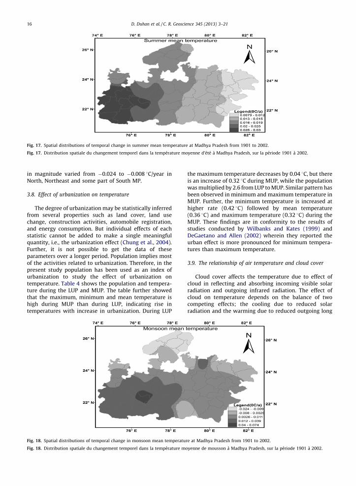
Fig. 15 shows the spatial distribution pattern oftemporal changes in the annual mean temperature. Similarto minimum and maximum temperature, the increase inmagnitude has been observed in annual mean temperatureover entire MP. The magnitude of annual mean tempera-ture varied from 0.0001 to 0.0070 8C/year in almost all overthe MP but drastically higher (0.02 to 0.08 8C/year) in somepart of the Chhatarpur, Panna and Dhindhol stations. Thewinter season (Fig. 16) also shows the increasing trend,which varied from 0.001 to 0.01 8C/year over the MP, but itexceeded 0.01 8C/year in some part of Rewa district. Insummer season (Fig. 17) also, the increase in magnitudewas observed which varied from 0.008 to 0.03 8C/year fromeast to west MP. During the monsoon season (Fig. 18), thespatial distribution of mean temperature can be charac-terized by a decline from west-south MP to northeast MP.The increase in magnitude varied from 0.0025 to 0.07 8C/year in west and central part of MP. However, the decrease
15. Spatial distribution of temporal change in the annual mean temperature at Madhya Pradesh from 1901 to 2002.
15. Distribution spatiale du changement temporel dans la temperature moyenne annuelle, a Madhya Pradesh, sur la periode 1901 a 2002.
16. Spatial distributions of temporal change in winter mean temperature at Madhya Pradesh from 1901 to 2002.
16. Distribution spatiale du changement temporel dans la temperature moyenne d’hiver a Madhya Pradesh, sur la periode 1901 a 2002.
D. Duhan et al. / C. R. Geoscience 345 (2013) 3–2116
in magnitude varied from �0.024 to �0.008 8C/year inNorth, Northeast and some part of South MP.
3.8. Effect of urbanization on temperature
The degree of urbanization may be statistically inferredfrom several properties such as land cover, land usechange, construction activities, automobile registration,and energy consumption. But individual effects of eachstatistic cannot be added to make a single meaningfulquantity, i.e., the urbanization effect (Chung et al., 2004).Further, it is not possible to get the data of theseparameters over a longer period. Population implies mostof the activities related to urbanization. Therefore, in thepresent study population has been used as an index ofurbanization to study the effect of urbanization ontemperature. Table 4 shows the population and tempera-ture during the LUP and MUP. The table further showedthat the maximum, minimum and mean temperature ishigh during MUP than during LUP, indicating rise intemperatures with increase in urbanization. During LUP
the maximum temperature decreases by 0.04 8C, but thereis an increase of 0.32 8C during MUP, while the populationwas multiplied by 2.6 from LUP to MUP. Similar pattern hasbeen observed in minimum and maximum temperature inMUP. Further, the minimum temperature is increased athigher rate (0.42 8C) followed by mean temperature(0.36 8C) and maximum temperature (0.32 8C) during theMUP. These findings are in conformity to the results ofstudies conducted by Wilbanks and Kates (1999) andDeGaetano and Allen (2002) wherein they reported theurban effect is more pronounced for minimum tempera-tures than maximum temperature.
3.9. The relationship of air temperature and cloud cover
Cloud cover affects the temperature due to effect ofcloud in reflecting and absorbing incoming visible solarradiation and outgoing infrared radiation. The effect ofcloud on temperature depends on the balance of twocompeting effects; the cooling due to reduced solarradiation and the warming due to reduced outgoing long
Fig. 17. Spatial distributions of temporal change in summer mean temperature at Madhya Pradesh from 1901 to 2002.
Fig. 17. Distribution spatiale du changement temporel dans la temperature moyenne d’ete a Madhya Pradesh, sur la periode 1901 a 2002.
Fig. 18. Spatial distributions of temporal change in monsoon mean temperature at Madhya Pradesh from 1901 to 2002.
Fig. 18. Distribution spatiale du changement temporel dans la temperature moyenne de mousson a Madhya Pradesh, sur la periode 1901 a 2002.
wabetandanncovannfoutemcortemcortemandsumshocov
4. D
varvarfor
theannannthein cet a(20havtemcauminclouthetemsamminfou
Tab
Pop
Tabl
Pop
P
LU
M
Tmax
Tab
Corr
Tabl
Coe
Va
Tm
Tm
Tm
Tmaxa
D. Duhan et al. / C. R. Geoscience 345 (2013) 3–21 17
ve radiation. Table 5 shows the correlation coefficientsween temperature variables (the mean, the maximum
the minimum temperatures) and cloud cover onual and seasonal basis. It can be seen that total clouder is negatively related with temperature variables inual and monsoon basis. However, a positive relation isnd in winter and summer season. The annual maximumperature shows the maximum significant negative
relation with cloud cover (�0.30) followed by meanperature (�0.26). In monsoon season, strong negative
relation is depicted between cloud cover and meanperature (�0.42) followed by the maximum (�0.41)
the minimum temperature (�0.40). Further, inmer season, only minimum temperature (0.26)
wed the significant positive correlation with clouder.
iscussion
The present study deals with an examination ofiability and trends in annual and seasonal temperatureiables (maximum, minimum and mean temperatures)the 45 stations of MP, in central India. It was found thatre are significant increases of 0.62 8C/102 years in theual minimum temperature, 0.60 8C/102 years in theual maximum temperature and 0.60 8C/100 years in
annual mean temperature over MP. These findings areonformity to the results of studies conducted by Karll. (1993), Qiang et al. (2004) and Wibig and Glowicki02) which have shown that minimum temperaturese increased much more rapidly than the maximumperatures. Henderson-Sellers (1995) reported that theses of differential increase in the maximum and theimum temperatures are closely related to change indiness. Seasonal analysis showed that magnitudes of
positive trends in winter, summer and monsoon meanperature were 1.20, 0.59 and 0.07 8C, respectively. Thee pattern has been observed in maximum andimum temperatures but the night temperature is
nd to be increasing more rapidly than day temperature.
These results are following the same trend as over India(Arora et al., 2005; Kothawale and Rupa Kumar, 2005; Pantand Kumar, 1997). Pant and Kumar (1997) reported asignificant warming trend of 0.57 8C per hundred years.Arora et al. (2005) also reported a significant increasingtrend over India during the years 1940 to 2000 at the rateof 0.42, 0.92 and 0.09 8C/100 years in annual meantemperature, mean maximum temperature and meanminimum temperature, respectively. Further, presentstudy findings are also consistent with the results ofKothawale and Rupa Kumar (2005), wherein they reportedthe significantly increase by 0.5 8C in annual meantemperature over India during the period of 1901 to2003. Analysis on monthly time step indicates thesignificant warming trend in the months of February,March, April, October, November and December in themean, the minimum and the maximum temperaturesduring the analysis period of 1901 to 2002. The increase intemperature during reproductive, grain formation andripening phase of crops (February to March) is understoodto be detrimental to productivity of wheat and other Rabiseason crops due to terminal stress. The decadal variationof annual temperature variables shows that the tempera-ture anomaly was positive after the 1951 to 1960 decade.The winter season mean temperature for sowing of Rabicrops in October to November was increased which can bedetrimental for seed germination. Similarly for Rabi cropsin reproductive phase (March to April) it may causehastening in the maturity, reduce grain setting and grainnumber, and thereby reduce yield. Crops like wheat andchickpea suffer from higher temperature, particularlyduring grain filling. Soybean is the main crop grown on77% of all agricultural land in MP. Lal et al. (1999) reportedthat if the maximum and minimum temperatures go up by1 8C and 1.5 8C respectively, the gain in yield comes downto 35%. Further, they also reported that if maximum andminimum temperatures rise by 3 8C and 3.5 8C respective-ly, then soybean yields will decrease by 5% compared to1998. This may ultimately affect the food security andeconomy of state and country.
le 4
ulation and temperature during less urbanized and more urbanized period.
eau 4
ulation et temperature pendant les periodes de moindre urbanisation et d’urbanisation plus prononcee.
Population Tmax (rate of change) Tmin (rate of change) Tmean (rate of change)
P 15,542,150 31.97 (�0.04) 18.75 (�0.03) 24.79 (�0.03)
UP 40,063,461 32.30 (0.32) 19.07 (0.42) 25.11 (0.36)
: maximum temperature; Tmin: minimum temperature; Tmean: mean temperature range; LUP: less urbanized period; MUP: more urbanized period.
le 5
elation coefficients of cloud cover with maximum temperature, minimum temperature and mean temperature range from 1901 to 2002.
eau 5
fficients de correlation entre couverture nuageuse et domaines de temperatures maximum, minimum et moyenne sur la periode 1901 a 2002.
riables Annual Winter Summer Monsoon
ax �0.30a 0.10 0.12 �0.41a
in �0.19 0.12 0.26a �0.40a
ean �0.26a 0.12 0.19 �0.42a
: maximum temperature; Tmin: minimum temperature; Tmean: mean temperature range.
Denote correlation that is significant at 5% significance level using the Kendall-tau method.
D. Duhan et al. / C. R. Geoscience 345 (2013) 3–2118
5. Conclusions
The conclusions drawn from the study are as follows:
� the significant increase in annual temperature is 0.62 8C(102 years)�1 in the minimum temperature, 0.60 8C (102years)�1 in the maximum temperature and 0.60 8C (102years)�1 in the mean temperature over MP;� seasonally, increase in magnitudes is 1.20, 0.59 and
0.07 8C in winter, summer and monsoon mean tempera-ture, respectively. The same pattern has been observedin maximum and minimum temperatures but the nighttemperature is found to be increasing more rapidly thanday temperature;� decadal variation of annual temperature shows that the
warming trends have begun from 1961 onward;� analysis on monthly time step indicates the significant
warming trend in the months of February, March, April,October, November and December in the mean, theminimum and the maximum temperature during theanalysis period of 1901 to 2002;� the minimum temperature is increased at higher rate
(0.42 8C) followed by the mean (0.36 8C) and the maxi-mum temperature (0.32 8C) during the MUP withincreased in population by around 2.6 fold from LUP toMUP;� further, cloud cover is significantly negatively related
with temperature variables in monsoon season and as awhole of the year. However, in summer season, positivecorrelation is found between cloud cover and tempera-ture variables.
Acknowledgements
The authors are thankful to the Department of Scienceand Technology (DST), New Delhi for providing financialsupport during the study period. We are also thankful toanonymous reviewers for their thoughtful suggestions toimprove this manuscript significantly.
Appendix
Detrended Fluctuation Analysis (DFA) method
DFA used in various time series (Chen et al., 2002; Maraun
et al., 2004; Peng et al., 1994; Varotsos, 2005a, b; Varotsos and
Cracknell, 2004; Weber and Talkner, 2001) to detect possible
long-range correlations consist of the following steps:
1. The first step is to integrate the given time series x(i) of
length N and construct the new time series using the
equation below:
y1 ¼ x1 � xavg ;
y2 ¼ x1 � xavg
� �þ x2 � xavg
� �y3 ¼ x1 � xavg
� �þ x2 � xavg
� �þ x3 � xavg
� �;
yN ¼XN
i¼1
xi � xavg
� �(1)
where, xavg ¼ 1N
PNi ¼ xi
The integration exaggerates the non-stationarity of the
original data, reduces the noise level, and generates a time
series corresponding to the construction of a random walk
that has the values of the original time series as increments.
The new time series, however, still preserves information
about the variability of the original time series (Kantelhardt
et al., 2002; Varotsos and Kirk-Davidoff, 2006).
2. Next step is to divide the time series y(i) into ‘m’ non-
overlapping segments of equal length d. For DFAn, in each
segment ‘m’ a best fit polynomial trend pnd,m of order n is
subtracted from the integrated y(i) time series:
yi ¼ y ið Þ � pnd;m ið Þ (2)
When linear polynomials are used, the fluctuation
analysis is called DFA1, for quadratic polynomials DFA2,
for cubic polynomials DFA3, etc. By definition, DFA2 removes
quadratic trends in the profile Y(i) and thus linear trends in
the original series xi.
3. Calculate the fluctuation function F(s) for each segment
If the r1 value falls within the confidence interval given
ve, the data are assumed to be serially independent
erwise the sample data are considered to be significant
ally correlated.
nn–Kendall test
The MK test, also called Kendall’s tau test due to Mann
45) and Kendall (1975), is the rank-based nonparametric
for assessing the significance of a trend, and has been
ely used in hydrological trend detection studies. It is
ed on the test statics S defined as:
Xn�1
i¼1
Xn
j¼iþ1
sgn x j � xi
� �(6)
ere x1, x2, . . ., xn represent n data points where xj
resents the data point at time j.
A very high positive value of S is an indicator of an
easing trend, and a very low negative value indicates a
reasing trend.
x j � xi
� �¼
1 . . . . . . . . . if x j � xi
� �> 0
0 . . . . . . . . . if x j � xi
� �¼ 0
�1 . . . . . . . . . if x j � xið Þ < 0
8<:
9=; (7)
It has been documented that when n � 10, the statistic S is
roximately normally distributed with the mean
Þ ¼ 0 (8)
its variance is
Sð Þ ¼ n n � 1ð Þ 2n þ 5ð Þ �P
ti ti � 1ð Þ 2ti þ 5ð Þ18
(9)
ere n is the number of data points, m is the number of groups (a tied group is a set of sample data having thee value), and ti is the number of data points in the ith
up.
The standardized test statistic Z is computed by as
ows:
Z ¼
S � 1ffiffiffiffiffiffiffiffiffiffiffiffiffiffiffiffiVAR Sð Þ
p if S > 0
0 if S ¼ 0S þ 1ffiffiffiffiffiffiffiffiffiffiffiffiffiffiffiffiVAR Sð Þ
p if S < 0
8>>>>><>>>>>:
9>>>>>=>>>>>;
(10)
The null hypothesis, H0, meaning that no significant trend
is present, is accepted if the test statistic Z is not statistically
significant, i.e. �Za/2< Z < Za/2, where Za/2 is the standard
normal deviate.
Theil–Sen’s estimator
The slope of n pairs of data points was estimated using the
Theil–Sen’s estimator (Theil, 1950 and Sen, 1968) that is
given by the following relation:
b ¼ Medianx j � xi
j � i
� �for all i < j (11)
In which 1 < j < i < n and b is the robust estimate of the
trend magnitude. A positive value of b indicates an ‘upward
trend’, while a negative value of b indicates a ‘downward
trend’.
Trend-free pre-whitening
The TFPW-MK procedure of Yue et al. (2002) is applied in
the following manner to detect a significant trend in a serially
correlated time series.
1. The slope (b) of a trend in sample data is estimated
using the approach proposed by Theil (1950) and Sen (1968).
The original sample data Xt were unitized by dividing each of
their values with the sample mean E(Xt) prior to conducting
the trend analysis (Yue et al., 2002). By this treatment, the
mean of each data set is equal to one and the properties of the
original sample data remain unchanged. If the slope is almost
equal to zero, then it is not necessary to continue to conduct
trend analysis. If it differs from zero, then it is assumed to be
linear, and the sample data are detrended by:
X0t ¼ Xt � Tt ¼ Xt � b � t (12)
2. The lag-1 serial correlation coefficient (r1) of the
detrended series Xt is computed using Eq. (5). If r1 is not
significantly different from zero, the sample data are
considered to be serially independent and the MK test is
directly applied to the original sample data. Otherwise, it is
considered to be serially correlated and AR (1) is removed
from the X0t by
Y 0t ¼ X0t � r1 � X 0t�1 (13)
This pre-whitening procedure after detrending the series
is referred to as the trend-free pre-whitening (TFPW)
procedure. The residual series after applying the TFPW
procedure should be an independent series.
D. Duhan et al. / C. R. Geoscience 345 (2013) 3–2120
3. The identified trend (Tt) and the residual Y0t are
combined as:
Yt ¼ Y 0t þ Tt (14)
The blended series (Yt) just includes a trend and a noise
and is no longer influenced by serial correlation. Then, the MK
test is applied to the blended series to assess the significance
of the trend.
References
Anderson, R.L., 1941. Distribution of the serial correlation coefficients.Ann. Math. Stat. 8 (1), 1–13.
Arora, M., Goel, N.K., Singh, P., 2005. Evaluation of temperature trendsover India. Hydrol. Sci. J. 50 (1), 81–93.
Ausloos, M., Ivanova, K., 2001. Power-law correlations in the southern-oscillation-index fluctuations characterizing El Nino. Phys. Rev. E. 63 ,http://dx.doi.org/10.1103/PhysRevE. 63047201 047201.
Batima, P., Natsagdorj, L., Gombluudev, P., Erdenetsetseg, B., 2005. Ob-served climate change in Mongolia. AIACC Working Paper 13, 25.
Bojkov, R.D., 1986. Surface ozone during the second half of the nineteenthcentury. J. Clim. Appl. Meteorol. 25, 343–352.
Boyles, R.P., Raman, S., 2003. Analysis of climate trends in North Carolina(1949–1998). Environ. Int. 29, 263–275.
Bozo, L., Weidinger, T., 1995. Tropospheric ozone measurements overHungary in the 19th century. Ambio. 23 (2), 129–130.
Cartalis, C., Varotsos, C., 1994. Surface ozone in Athens, Greece, at thebeginning and at the end of the 20th century. Atmos. Environ. 28, 3–8.
Chattopadhyay, S., Jhajharia, D., Chattopadhyay, G., 2011. Univariatemodelling of monthly maximum temperature time series over North-east India: neural network versus Yule-Walker equation based ap-proach. Meteorol. Appl. 18, 70–82.
Chen, Z., Ivanov, P.C., Hu, K., Stanley, H.E., 2002. Effect of non-stationa-rities on detrended fluctuation analysis. Phys. Rev. E. 65 , http://dx.doi.org/10.1103/PhysRevE.65.041107 041107.
Chung, U., Choi, J., Yun, J.I., 2004. Urbanization effect on the observedchange in mean monthly temperatures between 1951–1980 and1971–2000 in Korea. Clim. Change 66, 127–136.
Cohen, S., Stahill, G., 1996. Contemporary climate change in the Jordanvalley. J. Appl. Meteorol. 35, 1051–1058.
Cruz, R.V.O., Lasco, R.D., Pulhin, J.M., Pulhin, F.B., Garcia, K.B., 2006.Climate change impact on water resources in Pantabangan Water-shed, Philippines. AIACC Final Technical Report 9–107., http://www.aiaccproject.org/FinalReports/final_reports.htm.
Darshana, Pandey, A., 2013. Statistical analysis of long term spatial andtemporal trends of precipitation during 1901-2002 at Madhya Pra-desh. India. Atmos. Res. 122, 136–149.
Dash, S.K., Jenamani, R.K., Kalsi, S.R., Panda, S.K., 2007. Some evidence ofclimate change in twentieth-century India. Clim. Change 85, 299–321.
De, U.S., Mukhopadhyay, R.K., 1998. Severe heat wave over the Indiansubcontinent in 1998, in perspective of global climate. Curr. Sci. 75,1308–1311.
DeGaetano, A.T., Allen, R.J., 2002. Trends in twentieth-century extremesacross the United States. J. Climate 15, 3188–3205.
Dhorde, A., Dhorde, A., Gadgil, A.S., 2009. Long-term temperature trendsat four largest cities of India during the twentieth century. J. IndianGeophys. Union 13 (2), 85–97.
Easterling, D.R., Horton, B., Jones, P.D., Peterson, T.C., Karl, T.R., Parker,D.E., Salinger, J.M., Razuvzyev, V., Plummer, N., Jamason, P., Folland,C.K., 1997. Maximum and minimum temperature trends for the globe.Science 227, 364–365.
Eichner, J.F., Koscielny-Bunde, E., Bunde, A., Havlin, S., Schellnhuber, H.J.,2003. Power-law persistence and trends in the atmosphere: a de-tailed study of long temperature records. Phys. Rev. E. 68 , http://dx.doi.org/10.1103/Phys-RevE.68.046133 046133.
E.P.A., 1993. Air Quality Criteria for Ozone and Related PhotochemicalOxidants. Vol. I–III. External Review Drafts. US Environmental Pro-tection Agency, Washington, D.C (EPA-6001P-93-004 aF-cF).
Fuhrer, J., Skarby, L., Ashmore, M.R., 1997. Critical levels for ozone effectson vegetation in Europe. Environ. Pollut. 97, 91–106.
Gadgil, A., Dhorde, A., 2005. Temperature trends in twentieth century at
Galmarini, S., Steyn, D.G., Ainslie, B., 2004. The scaling law relatingworld point-precipitation records to duration. Int. J. Climatol. 24 (5),533–546.
Gemmer, M., Becker, S., Jiang, T., 2004. Observed monthly precipitationtrends in China 1951–2002. Theory Appl. Climatol. 77, 39–45.
Haan, C.T., 2002. Statistical Methods in Hydrology (second version).Blackwell Publishing, Iowa State Press, Ames, Iowa, pp. 496.
Helsel, D.R., 1987. Advantages of nonparametric procedures for analysisof water quality data. J. Hydrol. Sci. 32 (2), 179–190.
Henderson-Sellers, A., 1995. Future climates of the world: a modelingperspective. World Surv. Climatol. 16, 1–608.
Ichikawa, A. (Ed.), 2004. Global warming – The Research Challenges: AReport of Japan’s Global Warming Initiative. Springer, Berlin, 160 p.
IPCC, 2007. Impacts, Adaptation and Vulnerability. Contribution of Work-ing Group II. In: Parry, M.L., Canziani, O.F., Palutikof, J.P., van derLinden, P.J., Hanson, C.E. (Eds.), Fourth Assessment Report of theIntergovernmental Panel on Climate Change. Cambridge UniversityPress, Cambridge, UK, pp. 541–580.
Ivanov, P.C., Amaral, L.A.N., Goldberger, A.L., Havlin, S., Rosenblum, M.G.,Stanley, H.E., Struzik, Z.R., 2001. From 1/f noise to multifractal cas-cades in heartbeat dynamics. Chaos 11, 641–652.
Jaffe, D.A., Parrish, D., Goldstein, A., Price, H., Harris, J., 2003. Increasingbackground ozone during spring on the west coast of North America. J.Geophys. Res. 30 (12), 1613, http://dx.doi.org/10.1029/2003GL017024.
Ji, Y., Zhou, G., 2011. Important factors governing the incompatible trendsof annual pan evaporation: evidence from a small scale region. Clim.Change 106, 303–314.
Jung, H.S., Choi, Y., Oh, J.H., Lim, G.H., 2002. Recent trends in temperatureand precipitation over South Korea. Int. J. Climatol. 22, 1327–1337.
Kantelhardt, J.W., Zschiegner, S.A., Koscielny-Bunde, E., Havlin, S., Bunde,A., Stanley, H.E., 2002. Multifractal detrended fluctuation analysis ofnonstationary time series. Physica. A. 316 (1–4), 87–114.
Karl, T.R., Jones, P.D., Knight, R.W., Kukla, G., Plummer, N., Razuvayev, V.,Gallo, K.P., Lindseay, J., Charlson, R.J., Peterson, T.C., 1993. A newperspective on recent global warming: asymmetric trends of dailymaximum and minimum temperature. Bull. Am. Meteorol. Soc. 74,1007–1023.
Karnosky, D.F., Pregitzer, K.S., Zak, D.R., Kubiska, N.E., Hendrey, G.R.,Weinstein, D., Nosal, M., Percy, K.E., 2005. Scaling ozone responsesof forest trees to the ecosystem level in a changing climate. Plant, CellEnviron. 28, 965–981.
Kendall, M.G., 1975. Rank Correlation Methods, 4th ed. Charles Griffin,London, 202 p.
Kiehl, J.T., Trenberth, K.E., 1997. Earth’s annual global mean energybudget. Bull. Am. Meteorol. Soc. 78 (2), 197–208.
Kiraly, A., Bartos, I., Janosi, I.M., 2006. Correlation properties of dailytemperature anomalies over land. Tellus 58A (5), 593–600, http://dx.doi.org/10.1111/j.1600-0870.2006.00195.x.
Kondratyev, K.Y., Varotsos, C.A., 2001a. Global tropospheric ozone dy-namics. Part I: troposopheric ozone precursors. Environ. Sci. Pollut.Res. 8, 57–62.
Kondratyev, K.Y., Varotsos, C.A., 2001b. Global tropospheric ozone dy-namics. Part II: numerical modelling of tropospheric ozone variabili-ty. Environ. Sci. Pollut. Res. 8, 113–119.
Koscielny-Bunde, E., Bunde, A., Havlin, S., Roman, H.E., Goldreich, Y.,Schellnhuber, H.J., 1998. Indication of a universal persistence lawgoverning atmospheric variability. Phys. Rev. Lett. 81 (3), 729–732.
Kothawale, D.R., Rupa Kumar, K., 2005. On the recent changes in surfacetemperature trends over India. Geophys. Res. Lett. 32 (L18714), 4PP,http://dx.doi.org/10.1029/2005GL023528.
Lal, M., Singh, K.K., Srinivasan, G., Rathore, L.S., Naidu, D., Tripathi, C.N.,1999. Growth and yield responses of soybean in Madhya Pradesh,India to climate variability and change. Agric. Forest Meteorol. 93, 53–70.
Lee, S.H., Akimoto, H., Nakane, H., Kurnosenko, S., Kinjo, Y., 1998. Lowertropospheric ozone trend observed in 1989–1997 at Okinawa, Japan.Geophys. Res. Lett. 25, 1637–1640.
Lisac, I., Grubisic, V., 1991. An analysis of surface ozone data measured atthe end of the 19th-century in Zagreb, Yugoslavia. Atmos. Environ. 25,481–486.
Luterbacher, J., Dietrich, D., Xoplaki, E., Grosjean, M., Wanner, H., 2004.European seasonal and annual temperature variability. TrendsExtremes Sci. 303 (5663), 1499–1503.
Madnani, G.M.K., 2009. Introduction to Econometrics: Principles andApplications, 8/E. Oxford and IBH, Publishing Co. Pvt. Ltd., New Delhi,p. 1–451.
Mann, H.B., 1945. Non-parametric test against trend. Econometrica 13,245–259.
Maraun, D., Rust, H.W., Timmer, J., 2004. Tempting long-memory – on the
interpretation of DFA results. Nonlin. Proc. Geoph. 11, 495–503. Pune, India. Atmos. Environ. 39, 6550–6556.
D. Duhan et al. / C. R. Geoscience 345 (2013) 3–21 21
selman, R.C., Massman, W.J., 1999. Ozone flux to vegetation and itsrelationship to plant response and ambient air quality standards.Atmos. Environ. 33, 65–73.olls, N., Collins, D., 2006. Observed change in Australia over the past
century. Energy Environ. 17, 1–12.e, M., Ellul, R., Ventura, F., Gusten, H., 2005. A study of historicalsurface ozone measurements (1884–1900) on the island of Gozo inthe central Mediterranean. Atmos. Environ. 39, 5608–5618.renshaw, J.H., Lyons, T., Barnes, J.D., 1999. Impacts of ozone on growthand yield of field grown oilseed rape. Environ. Pollut. 104, 53–57.
ans, S.J., Lefohn, A.S., Scheel, H.E., Harris, J.M., Levy, H., Galbally, I.E.,Brunke, E.G., Meyer, C.P., Lathrop, J.A., Johnson, B.J., Shadwick, D.S.,Cuevas, E., Schmidlin, F.J., Tarasick, D.W., Claude, H., Kerr, J.B., Uchino,O., Mohnen, V., 1998. Trends of ozone in the troposphere. Geophys.Res. Lett. 25, 139–142.t, G.B., Kumar, K.R., 1997. Climates of South Asia. John Wiley & SonsLtd, Chichester, UK, 320 p.g, C.K., Buldyrev, S.V., Havlin, S., Simons, M., Stanley, H.E., Goldberger,A.L., 1994. Mosaic organization of DNA nucleotides. Phys. Rev. E. 49(2), 1685–1689.rson, B.J., Holmes, R.M., McClelland, J.W., Vorosmarty, C.J., Lammers,R., Shiklomanov, A.I., Shiklomanov, I.A., Rahmstorf, S., 2002. Increas-ing river discharge to the Arctic Ocean. Science 298, 137–143.s, J.C.M., Alvim-Ferraz, M.C.M., Martins, F.G., 2012. Surface ozonebehaviour at rural sites in Portugal. Atmos. Res. 104–105, 164–171.g, F., Celeste, M.J., Stephen, G.W., Dian, J.S., 2004. Contribution of
stratospheric cooling to satellite inferred tropospheric temperaturetrends. Nature 429, 55–57.anathan, V., Feng, Y., 2009. Air pollution, greenhouse gases and
climate change: global and regional perspectives. Atmos. Environ.43, 37–50.anathan, V., Ramana, M.V., Roberts, G., Kim, D., Corrigan, C., Chung, C.,
Winker, D., 2007. Warming trends in Asia amplified by brown cloudsolar absorption. Nature 448, 575–578.lieva, I.P., Semiletov, L.N., Vasilevskaya, Pugach, S.P., 2000. A climate
shift in seasonal values of meteorological and hydrological param-eters for northeastern Asia. Prog. Oceanogr. 47, 279–297.
P.K., 1968. Estimates of the regression coefficient based on Kendall’stau. J. Am. Stat. Assoc. 63, 1379–1389.Y.F., Shen, Y.P., Hu, R.J., 2002. Preliminary study on signal, impact andforeground of climatic shift from warm-dry to warm-humid inNorthwest China. J. Glaciol. Geocryol. 24, 219–226.a Ray, K.C., De, U.S., 2003. Climate change in India as evidenced frominstrumental records. WMO Bull. 52 (1), 53–59.dt, S., Herman, F., 2004. Evaluation of air pollution related risks forAustrian mountain forests. Environ. Pollut. 130, 99–112.ers, R., 1992. On the statistical analysis for the objective determina-
tion of climate change. Meteorol. Z.N.F. 1, 247–256.ani, E., Soltani, A., 2008. Climatic change of Khorasan, North-East ofIran, during 1950–2004. Res. J. Environ. Sci. 2 (5), 316–322.helin, J., Thudium, J., Buehler, R., Volz-Thomas, A., Graber, W., 1994.Trends in surface ozone concentrations at Arosa (Switzerland).Atmos. Environ. 28 (1), 75–87.
Stanley, E., 1999. Scaling, universality, and renormalization: three pillarsof modern critical phenomena. Rev. Mod. Phys. 71 (2), S358–S366.
Tabari, H., Hosseinzadeh Talaee, P., 2011. Recent trends of mean maxi-mum and minimum air temperatures in the western half of Iran.Meteorol. Atmos. Phys. 111, 121–131.
Talkner, P., Weber, R.O., 2000. Power spectrum and detrended fluctuationanalysis: application to daily temperatures. Phys. Rev. E. 62 (1), 150–160.
Theil, H., 1950. A rank invariant method of linear and polynomial regres-sion analysis, part 3. Netherlands Akademie van Wettenschappen,proceedings, 53, pp. 1397–1412.
Tsonis, A., Roeber, P., Elsner, J., 2000. On the existence of spatially uniformscaling laws in the climate system. In: Novak, M. (Ed.), Paradigms ofComplexity. World Scientific, Singapore, pp. 25–28.
Varotsos, C., Cartalis, C., Vlamakis, A., Tzanis, C., Keramitsoglou, I., 2004.The long-term coupling between column ozone and tropopauseproperties. J. Climate 17, 3843–3854.
Varotsos, C., 2005a. Power law correlations in column ozone overAntarctica power law correlations in column ozone over Antarctica.Int. J. Remote Sens. 26 (16), 3333–3342.
Varotsos, C., 2005b. Modern computational techniques for environmentaldata: application to the global ozone layer. Computational science –ICCS 2005, PT 3 Book series: lecture notes in computer science 3516,pp. 504–510.
Varotsos, C.A., Cracknell, A.P., 2004. New features observed in the 11-yearsolar cycle. Int. J. Remote Sens. 25, 2141–2157.
Varotsos, C., Kirk-Davidoff, D., 2006. Long-memory processes in ozoneand temperature variations at the region 608 S–608 N. Atmos. Chem.Phys. 6, 4093–4100.
Vincent, L.A., Wijngaarden, W.A.V., Hopkinson, R., 2007. Surface temper-ature and humidity trends in Canada for 1953–2005. J. Climate 20,5100–5113.
Vingarzan, R., 2004. A review of surface ozone background levels andtrends. Atmos. Environ 38, 3431–3442.
Vingarzan, R., Thomson, B., 2004. Temporal variation in daily concentra-tions of ozone and acid related substances at Saturna Island, BritishColumbia, Canada. J. Air Waste Manage. Assoc. 54, 459–472.
Wallis, J.R., O’Connell, P.E., 1972. Small sample estimation of r1. WaterResour. Res. 8 (3), 707–712.
Weber, R.O., Talkner, P., 2001. Spectra and correlations of climate datafrom days to decades. J. Geophys. Res. 106, 20131–20144.
Wibig, J., Glowicki, B., 2002. Trends in minimum and maximum tempera-ture in Poland. Clim. Res. 20, 123–133.
Wilbanks, T.J., Kates, R.W., 1999. Global change in local places: how scalematters. Clim. Change 43 (3), 601–628.
Wilks, D.S., 2006. Statistical Methods in Atmospheric Sciences, 2nd ed.Academic Press, San Diego, California.
Yue, S., Pilon, P., Phinney, B., Cavadias, G., 2002. The influence of autocor-relation on the ability to detect trend in hydrological series. Hydrol.Processes 16, 1807–1829.
Zhang, X., Lucie, A., Vincent, W.D., Hogg-Niitsoo, A., 2000. Temperatureand precipitation trends in Canada during the 20th century. Atmos.–Ocean 38 (3), 395–492.