Journal of Agricultural and Resource Economics 40(3):442–456 ISSN 1068-5502Copyright 2015 Western Agricultural Economics Association

Spatial Competition, Arbitrage,and Risk in U.S. Soybeans

Kristopher Skadberg, William W. Wilson, Ryan Larsen, and Bruce Dahl

This paper analyzes spatial arbitrage and vertical integration of a U.S. soybean-trading firm. Arisk-constrained optimization model using Monte Carlo simulation and copula joint distributionsis specified. Results show that spatial-arbitrage payoffs vary regionally. Sensitivity results indicatethat payoffs and risks increase as firms become more vertically integrated.

Key words: copula, spatial arbitrage, spatial competition, trading strategies

Introduction

Many challenges confront commodity traders, including deciding where to buy and sell and howto manage transactions and logistics. These are compounded in soybean markets because therehas been increased volatility in basis, futures, and rates for all modes of transportation in recentyears (Prokopczuk and Simen, 2014; Wilson and Dahl, 2011). There is also intense intermarketcompetition, notably for shipments to the U.S. Gulf (USG) and the Pacific Northwest (PNW).Production has shifted, with more soybeans being produced in the upper Midwest. China is thetop U.S. soybean importer, accounting for up to 64% of U.S. soybean exports in recent years.Increased Asian demand has created congestion at ports, but expansion of port facilities in the PacificNorthwest has mitigated these constraints (Wilson and Dahl, 2011). Taken together, these changesare particularly important for northern soybean-growing states. Most important is the substantialgrowth in soybean production, which increased for North Dakota from 2.9 million acres in 2005 tonearly 6 million acres in 2014; exports from North Dakota have increased from 32 million bushelsin 2004 (Vachal and Benson, 2011) to 188 million bushels in 2014 (ProExporter). In 2015 NorthDakota will be the largest state net exporter of soybeans, and these exports are largely through thePacific Northwest. These changes have motivated research to more fully understand spatial arbitragein the soybean market.

The purpose of this study is to analyze spatial arbitrage for a trading firm handling soybeanswith terminal facilities in both the U.S. Gulf and Pacific Northwest. A risk-constrained optimizationmodel using Monte Carlo simulation with a copula joint distribution was specified to maximizearbitrage payoffs. The portfolio consists of origin and destination prices as well as shipping costsfor rail, barge, and ocean shipping. The model was solved assuming no vertical integration, andsensitivities were conducted to evaluate alternative vertical market strategies for the firm. Resultswere used to identify locations that have the greatest opportunities for spatial arbitrage as well asthe frequency of intermarket arbitrage. The results indicate that spatial-arbitrage payoffs vary acrossorigins. Results from the sensitivities indicate that increased vertical integration in the supply chaincorresponds to larger spatial-arbitrage payoffs and risk.

Kristopher D. Skadberg is former graduate student in Agribusiness and Applied Economics, William W. Wilson is a universitydistinguished professor, Ryan Larsen is assistant professor, and Bruce Dahl is research scientist, all at North Dakota StateUniversity.

Review coordinated by Larry Makus.

Skadberg et al. Spatial Competition, Arbitrage, and Risk 443

Background and Related Studies

Spatial price relationships in grains and commodity trading are determined primarily by the basisand transfer costs, which are primarily for shipping. Changes to either of these can alter commodityflows. When prices differ by more than the marketing costs, traders can earn spatial-arbitragepayoffs. Other costs, which vary across shippers and through time, are unobserved and include costsrelated to loading and unloading; demurrage; expertise and time; contracting; insurance; financing;and fees associated with testing, grading, and meeting phytosanitary standards.

Arbitrage refers to buying and selling commodities to take advantage of price differentials.Weisweiller (1986, pp. 1–10) provides many definitions for arbitrage, but all of these involveknowledge, foresight, and judgment. One of the most common forms of arbitrage in grain is spatialarbitrage, which involves buying grain at an origin, simultaneously selling at a destination, andaccruing the costs of shipping (Kub, 2014, p. 39). While spatial arbitrage is an age-old conceptand a function of trading firms, recent research has emphasized its importance. Simon (2015)reports several examples of simple commodity spatial arbitrage, while Pirrong (2014, p. 8) providesanalysis of the trading industries and indicates that “commodity trading firms are all essentiallyin the business of transforming commodities in space (logistics). . . / Their primary function is to‘perform physical arbitrages’ which enhance value through these various transformations.” In theprocess of arbitrage they conduct an “optimization process” (p. 8), accounting for shipping costs.Through this process, their core activity is bilateral search due to the randomness of critical variables,which is used to identify opportunities with the greatest arbitrage payoffs. The roles of informationand operations are therefore critical: “Commodity trading therefore involves the combination ofthe complementary activities of information gathering and analysis and the operational capabilitiesnecessary to respond efficiently to this information” (Pirrong, 2015). Meersman, Reichtsteiner, andSharp (2012) focus their discussion on the need for trading firms to transform from non-asset-basedtrading to more vertically integrated operations and show evidence that firms that have done socapture greater returns.

Nonlinear and stochastic transfer costs cause market boundaries to fluctuate over time. Othercritical risks are the random changes in basis at competing terminal markets and the randomness inshipping costs from each origin to each destination. Conceptually, traders arbitrage price differencesuntil markets have equal basis adjusted for shipping costs. In fact, location arbitrage is a “tradingstrategy to profit from market inefficiencies in price differences” (Simon, 2015). Arbitrage isthe process by which markets compete and become efficient in the long run, conforming to thelaw of one price, implying that markets for homogeneous products should function efficiently sothat any potential riskless payoffs through arbitrage trade are eliminated (Goodwin et al., 2011).Spatial arbitrage entails buying from underpriced and selling to overpriced spatially disparatemarkets to take advantage of price differentials. The process of spatial arbitrage has risk becauseof random elements (prices, shipping and other costs, etc.). Additionally, shipments cannot bedelivered instantaneously. Ultimately, spatial arbitrage reflects local supply and demand conditionsat that time (Kub, 2014). Random unobserved costs make it difficult to accurately value spatialarbitrage. However, forward contracts can be used to lock in destination-market prices, whichmitigate risks associated with noninstantaneous shipments. The law of one price is a longer-termconcept, though other studies have shown flaws in this concept in the short run (Ardeni, 1989; Isard,1977; Protopapadakis and Stoll, 1983; Thursby, Johnson, and Grennes, 1986).

Following Baulch (1997), the theoretical spatial-arbitrage equations are defined below:

(1) Bd > Bo + tr,

where Bd is the basis at the destination market (defined as the difference between local cash priceand futures contract price), tr is transfer costs from the origin to the destination market, and Bo isthe origin basis (local cash price minus futures price). In equation 1, spatial-arbitrage payoffs wouldexist. Use of basis in this evaluation is based on the assumption that traders are fully hedged in the

444 September 2015 Journal of Agricultural and Resource Economics

futures market. Equation (2) represents a case where there is no arbitrage opportunity:

(2) Bd = Bo + tr.

Equation (3) represents a case where no trade occurs from the export to the import market; however,an arbitrage opportunity could occur from the import to export market:

(3) Bd + tr < Bo.

Arbitrage does not work perfectly and, in most cases, carries varying levels of risk (Shleifer andVishny, 1997). Therefore, markets may remain inefficient until the risk is matched with a return. Ifthe markets continue to diverge, more capital is needed, and more risk is involved with the transfer.If an arbitrager can gain the same payoff with a lower amount of risk, he or she will choose the lessrisky trade (Ali, Hwang, and Trombley, 2003).

Several recent studies have analyzed spatial arbitrage in commodities. Simon (2015) providesnumerous simple examples of location arbitrage. Borenstein and Kellogg (2012) study the increasingspread between the West Texas Intermediate (WTI) oil price and Brent crude oil. Before theintroduction hydraulic fracturing (“fracking”), the WTI and Brent crude oil had small price spreads,but increased oil production in North Dakota overwhelmed the export pipeline from Cushing,Oklahoma, where the WTI oil price is derived (as explained in Gold and Friedman, 2013). Theexcess supply at Cushing lowered the WTI oil price and represented an arbitrage opportunity forselling oil to the export market. This study regresses price changes for crude oil and Midwest fuelprices. The arbitrage opportunity remained due to constraints in the supply chain, and oil refineriesin the upper Midwest benefited from the lower WTI oil price.

Park et al. (2002) investigate China’s infrastructure bottlenecks, managerial incentive reforms,and production-specialization policies, all of which are contributing factors affecting marketintegration in China’s grain markets. Their study uses a parity-bounds model (Spiller and Huang,1986; Sexton, Kling, and Carman, 1991; Baulch, 1997) to analyze whether the lack of integration,if any, is related to failed arbitrage, autarky, or trade-flow switching. Results indicated thatinexperienced traders, market maturity, and policies segmented across different regions creategreater arbitrage opportunities. Trade barriers had a smaller effect on market inefficiencies thanoriginally expected.

Empirical Methods

There are four steps to our empirical analysis. First, we specify a spatial-arbitrage model for asingle representative firm with export port elevators in the Pacific Northwest and U.S. Gulf thatis capable of buying soybeans from multiple origins throughout the U.S. Midwest. The analyticalspecification is adapted from a model of risk arbitrage (Winston, 2008, pp. 77–82). Second, wederive distributions of the relevant random variables, primarily prices at Gulf and PNW locations inaddition to each of the origins, and shipping costs. Many factors may cause changes in these values,including the level and expectations of outstanding export sales, export cancellations, competitionfrom competing exporting countries, Canadian grain imports which do not conform to country-of-origin specifications for phytosanitary certification, and impacts of industry concentration, changesin oil prices, and car placements (the effects of which are described in Wilson and Dahl, 2011). Froman individual firm perspective, it is reasonable to assume that these impacts are random and reflectedin changes in basis values. Third, we solve a base-case strategy that assumes the firm is verticallynon-integrated. Finally, we specify alternative vertical integration strategies to evaluate their impactsrelative to the base-case results. The results are compared based on returns and risk.

The fundamental relationship governing spatial market equilibrium can be expressed as

(4) π =∑dt

BdtQdt − ∑ort(Bot + trt)Qort ,

Skadberg et al. Spatial Competition, Arbitrage, and Risk 445

where Bdt = (B1t , B2t , . . . , Bdt) is the basis at destination d and time t. Variable Qdt represents thequantity sold at destination d at time t, Qort is the quantity of soybeans bought and shipped fromorigin o and transportation route r and time t, and Bot = (B1t , B2t , . . . , Bit) is the basis for buyingsoybeans at origin o and time t. Transportation costs are defined by trt = (t1t , t2t , . . . , trt), wheretrt represents the observed transfer costs for route r during time t. Transfer costs comprised manyvariables, the largest being transportation.

All elevators in the model are shuttle-loading facilities (Sarmiento and Wilson, 2005; Wilsonand Dahl, 2011).1 For this reason, shipping costs include tariff rates, rail car premiums, and fuelservice charges, all of which vary through time. Other variable costs are for storage, interest, riskpremiums, shrinkage, moisture loss, electricity for elevator functions and handling. Most of thenontransportation transfer costs are not observed and likely similar across plants. Due to the highlycompetitive industry for trading and handling and the fairly homogenous technology among shuttleelevators, differences across locations should be minimal. Regardless, these are not observed andhence were not included in the model. Technically, the Bot observed in our model is the price offeredto growers. Hence, ÏA is the payoff due to “spatial arbitrage and origination” that includes theseunobserved costs.2

An optimization model was specified based on a risk-constrained portfolio, which determinesthe weight for each origin that yields the maximum payoff from spatial arbitrage and origination.The first case examines spatial-arbitrage opportunities for shuttle loaders (shipping to a grain-tradingfirm with terminals in the U.S. Gulf and Pacific Northwest) specified as

MAXπ =D

∑d=1

BdQd +O

∑o=1

−BoQo +R

∑r=1

trQr

s.t. 0 ≤ Qd ≤ 8,740,032,

0 ≤ Qo ≤ 832,384,(5)

0 ≤ Qr ≤ 8,740,032,

π ≥ 0,

J

∑j=1

Qd −I

∑i=1

Qo = 0,

J

∑j=1

Qd −R

∑r=1

Qr = 0,

where Qd , Qo, and Qr are the decision variables representing the amount of soybeans (in bushels)sold, bought, and shipped, per week.3 In a simple case, buyers would buy from a single origin andship to one destination. However, given multiple origins, two destinations (USG and PNW), and theimpact of constraints on quantities, the results become more complex. Some origins ship by truck-barge and/or rail. The sum of these would equal Qo. From one origin, soybeans could be shippedto the Pacific Northwest by rail and also shipped by barge to the U.S. Gulf. This could happen ifthe Pacific Northwest reached its maximum capacity and an origin that had already shipped somebushels to the Pacific Northwest had positive payoffs for shipments to the U.S. Gulf to reach the

1 Shuttle elevators are approved to ship under “shuttle terms,” which include lower rates, priority loading, and the abilityto load and unload 110 cars in a specified, limited amount of time. Conforming facilities receive rate discounts, rebates, andvarying forms of developmental assistance. See Wilson and Dahl (2011) for a description of these mechanisms and measuresof their randomness.

2 While this is not perfect, it is the best that can be done with observable variables. The results are consistent with spatialarbitrage, but the interpretation is strictly as noted: returns to spatial arbitrage and origination.

3 An alternative would be to specify the model with Qr as the decision variable, which—subject to all arbitrageopportunities and capacity limits—would generate optimal Qo and Qd .

446 September 2015 Journal of Agricultural and Resource Economics

origin’s maximum loading capacity.4 Each of these variables would be similar to the optimizationprocess that trading firms use to identify spatial-arbitrage opportunities (Pirrong, 2014, p. 8).

The variable Bd represents the sale price to the grain-trading firm’s port elevators, quoted aseither the track or CIFNOLA basis at ports d = 1, 2, 3, . . . , D. The track basis is the price paidfor soybeans delivered to the terminal in a railcar and CIFNOLA is the price paid for soybeansdelivered to a New Orleans terminal. The variable Bo is the buying basis at o = 1, 2, 3, . . . , O,which represents prices paid to growers, and tr is the shipping costs for routes r = 1, 2, 3, . . . , R.

The model chooses from all origins and destinations when deciding where to ship soybeanson a weekly basis. One restriction is the number of bushels that can be handled per week, as .thetrading firm’s port facilities can only unload a limited number of bushels each week. The variableQd constrains the quantity bought at the port to between 0 and 8.7 million bushels per week, whichis the maximum that a typical port elevator can unload.

Other restrictions were included in the model. The combined purchases from the beginning andend of the week cannot exceed the equivalent of two shuttle trains per week. The amount of grainpurchased at the origin must equal the amount of grain sold at the ports. The decision variable, Qois the number of bushels to be bought at each origin. Taken together, we assume that each origin canload a maximum of two shuttle trains per week (832,384 bushels) and that the export elevator canload a maximum of 8.7 million bushels per week. These restrictions imply that the trader could buyfrom a maximum of 57% of the origins in any single week (or iteration). The remaining constraintsforce the arbitrager to sell the same amount thawt he or she purchases.

Equation (5) is the base case representing a non-vertically integrated firm that simultaneouslybuys soybeans at origins and sells at ports. In this scenario, the shuttle-loading firms are not exposedto basis risk, because the commodity is bought and sold simultaneously. We specify alternativestructures to evaluate strategies related to vertical integration. In this case, different representativeprices are included in equation (5). The first evaluates spatial-arbitrage opportunities for the grain-trading firm’s export terminals. Buying soybeans delivered to port terminals on a rail track orCIFNOLA basis (delivered by barge to a port terminal) and selling on a FOB basis (“Free on Board”an ocean-going vessel at the port elevator) is commonly termed FOBBING. The difference betweenthe purchase and sale values is the FOB margin. The sum of quantities sold at the ports must equalvolumes purchased from shuttle elevators. Traders have the ability to simultaneously buy track orCIFNOLA basis and to sell exports on a FOB basis value. Traders can buy soybeans at the beginningof the week and store the crop until they sell it at the end of the week. In this sensitivity, the basisvalues at the destination and origin in equation (5) are replaced and the shipping cost becomes nil.The destination basis becomes the FOB basis value at the port, and the origin basis is the track basisat the port.

The second alternative poses a vertically integrated grain-trading firm owning both domesticshuttle elevators and port terminals. The trader earns a margin by purchasing soybeans and shippingthem to its PNW or USG port terminals and selling them on a FOB basis. In this case, the destinationbasis values in equation (5) (track and barge bids) were replaced with the FOB basis values at theport for export shipment.

The next alternative represents a vertically integrated grain-trading firm that owns domesticorigins and port terminals and also sells cost and freight (C&F) (i.e., ships soybeans internationally).In this case, the derived prices and costs represent selling and shipping to C&F destinations in Asia.The vertically integrated firm owns shuttle and export elevators in addition to buying ocean freightand sells soybeans basis C&F. This sensitivity evaluates the potential payoff increase attributed to a

4 In the empirical model, the firm can handle 57% of potential shipments at best. Since we measure arbitrage plus thehandling margin, arbitrage opportunities can represent at best the top 57% of potential arbitrage opportunities or (at worst)may include origins sacrificing some or all of their margins. The model chooses those origins with the greatest payoffs andcontinues buying from those origins with positive payoffs up to the restriction. Each of these variables is important, and theoptimization process would be similar to the optimization process that trading firms go through to identify spatial-arbitrageopportunities (Pirrong, 2014, p.8). One of the restrictions applies to the point of unloading at the export. For this reason, someorigins may have positive payoffs but are lower than those of the 57% of origins with greater payoffs.

Skadberg et al. Spatial Competition, Arbitrage, and Risk 447

grain-trading company owning the most profitable locations. The amount of grain purchased at theorigin has to match the amount of grain loaded at the ports, the amount of ocean freight purchased,and the volume of exports sold. This constraint forces the model to behave as a vertically integratedfirm. In addition, the destination basis prices in equation (5) were replaced with the values equivalentof C&F Asia from each origin port.

Stochastic Optimization

The model was solved using stochastic optimization.5 Multivariate distributions with copuladependence structures were derived for origin and destination basis values and transportation costs(described below), from which we collected 10,000 sets of samples. Models were solved for theoptimal arbitrage opportunities for each set of samples. This procedure was repeated for each weekof the 10,000 sets of random draws. Using this procedure, we simulated first a base-case strategythat assumes the firm is nonintegrated. Then we simulated alternative vertical integration strategiesto evaluate their impacts relative to the base-case results. The results for these sensitivities arecompared based on returns and risk.

Data Sources and Distributions

Weekly basis values for thirty-seven Midwest shuttle facilities representative of soybean-producingregions were used for this research. Technically, these are basis bids offered to growers. WeeklyFOB, Track, and CIFNOLA basis values for the Pacific Northwest and U.S Gulf were used. Railrates and/or barge shipping costs were derived from each origin to the Pacific Northwest, U.S.Gulf, or both (BNSF). These values included tariff shipping rates, fuel service charges, and rail-car premiums.

The data were 2004–2009 weekly observations from the following sources: barge freightrates (U.S. Department of Agriculture, Agricultural Marketing Service, 2014; U.S. Department ofAgriculture, Agricultural Marketing Service, Transportation Service Division, 2014), rail freightrates (BNSF), CIFNOLA barge soybean basis (Advanced Trading, LLC), secondary rail-car values(TradeWest Brokerage), PNW rail soybean basis (Advanced Trading, LLC), rail fuel-surcharge rates(TradeWest Brokerage and BNSF), and origin basis price level (DTN). Ocean-shipping rates fromthe U.S. Gulf and Pacific Northwest to Asia were from the USDA-AMS Transportation ServiceDivision.

Randomness in these variables was captured using univariate marginal distributions and copuladependency measures. Univariate distributions were fitted for each of the basis at the ports and ateach origin, in addition to shipping costs. The results indicated that many of these were non-normal,though some were skewed to the right.6

Copula

Distributions were used to capture interdependencies among variables. Copula dependency measureshave been used in other spatial-market studies to test market integration for strand board (e.g.,Goodwin et al., 2011). Asymmetric dependency measures were used to allow more weight to beplaced on one tail of the marginal distribution.7 Symmetric dependency measures place equal weighton both tails of the marginal distribution. Copulas provide more flexible dependence measureswhen dealing with asymmetric dependences because no assumptions are placed on the marginaldistributions (Vose, 2008) and tail dependency can be incorporated.

5 Simon’s 2015 representation of the solution to spatial arbitrage refers to both an optimization problem and a stochasticproblem but does not apply the methodologies used here.

6 The volume of these univariate results is too extensive to present here but is available from the authors on request.7 See Nelsen (2006) for detailed definitions and proofs.

448 September 2015 Journal of Agricultural and Resource Economics

Table 1. Sample of Gaussian Copula Parameters among Basis by LocationVariables PNW US Gulf Albany Alden Alton Aurora Ayr Bayard BeatricePNW 1.00 0.50 0.39 0.42 0.52 0.32 0.48 0.40 0.38US Gulf 0.50 1.00 0.43 0.32 0.32 0.32 0.27 0.29 0.27Albany 0.39 0.43 1.00 0.57 0.48 0.63 0.47 0.58 0.56Alden 0.42 0.32 0.57 1.00 0.59 0.62 0.63 0.80 0.73Alton 0.52 0.32 0.48 0.59 1.00 0.45 0.75 0.62 0.63Aurora 0.32 0.32 0.63 0.62 0.45 1.00 0.51 0.65 0.60Ayr 0.48 0.27 0.47 0.63 0.75 0.51 1.00 0.66 0.66Bayard 0.40 0.29 0.58 0.80 0.62 0.65 0.66 1.00 0.78Beatrice 0.38 0.27 0.56 0.73 0.63 0.60 0.66 0.78 1.00

Table 2. Portfolio Payoffs

Payoff Std. Dev. Payoff 1/CV 5% Seven-Day VaR

Sensitivity ($ Millions) ($ Millions) ($/bu) ($ Millions)

Base Case $3.6 $2.3 $0.12 1.55Sell FOB/Buy Track $2.3 $3.3 $0.07 0.72 $(1.4)Vert. Int. w/o Ocean $6.5 $4.8 $0.22 1.37 $(4.9)Vert. int. w/ Ocean $9.7 $11.4 $0.33 0.85 $(9.5)

In this analysis, a large number of shipping costs were highly correlated, which required analternative specification. Random shipping costs were included for the three main routes (a baseorigin to the U.S. Gulf via rail, to the U.S. Gulf via barge, and to the Pacific Northwest). Differentialsfor alternative routes were derived as the difference between the comparable base route and the ratefor the alternative route. Then the copula dependence was estimated with the random shipping costsfor the three routes and other random variables. This process simplified the estimation of the copulaparameters. There were still a large number of remaining variables; as such, the estimated copulaconverges from a Student t to a Gaussian copula (Vose, 2008), which is what was used. The deriveddifferentials were later applied to the simulated weekly base rates to determine shipping costs foreach origin/destination movement for that week.

Maximum likelihood estimation was used to estimate the copula (Nelsen, 2006) using thefollowing equation:

(6) δ2 = argmaxδ2

T

∑t=1

lnc(Gx(xt), Hy(yt),δ2),

where δ2 is the estimated copula parameter and (Gx(xt), Hy(yt),δ2) is the estimated marginaldistribution for x and y. Parameters for all copulas are estimated using SAS. Scatterplots for thetransformed data for selected origins are illustrated in figure 1 with the estimated Gaussian copula.

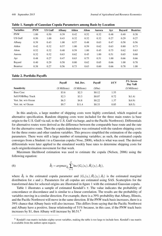
Table 1 illustrates a sample of estimated Kendall’s τ . The value indicates the probability ofconcordance or discordance and is similar to a linear correlation. The results are the probability ofvariables moving in a similar direction. For example, there is a 39% probability that Albany, Illinois,and the Pacific Northwest will move in the same direction. If the PNW track basis increases, there is a39% chance that Albany basis will also increase. This differs from saying that the Pacific Northwestand Albany have a positive, linear relationship of 51% because, in this case, if the PNW track basisincreases by $1, then Albany will increase by $0.51.8

8 Kendall’s tau matrix includes eighty-seven variables, making the table is too large to include here. Kendall’s tau matrixis available from the authors upon request.

Skadberg et al. Spatial Competition, Arbitrage, and Risk 449

Figure 1. Empirical Margins, Gaussian Copula Scatter-Plot Matrix

Results

Table 2 shows evaluations for spatial payoffs due to arbitrage and origination (hereafter referredsimply as arbitrage payoffs). Arbitrage payoffs averaged $3.6 million ($0.12/bu) across origins.The variability of arbitrage payoffs had a standard deviation of $2.3 million ($0.08/bu), and theestimated ratio for 1/CV was 1.55, indicating the payoffs for each unit of risk. This indicates thatthere are significant spatial-arbitrage opportunities for independent shuttle operators, which have alow proportion of variability in relation to returns.

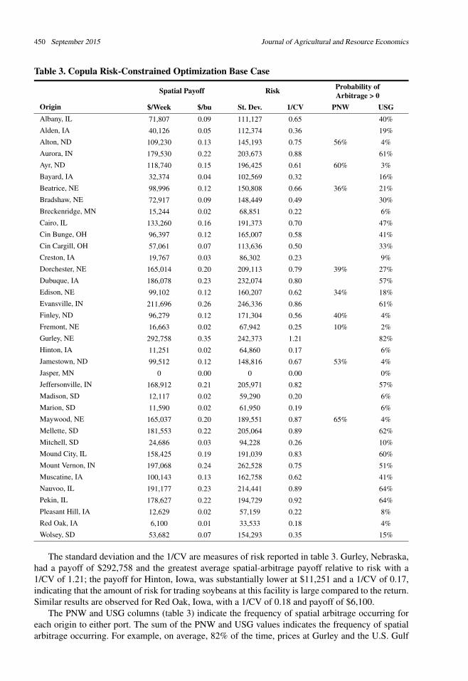
Spatial-arbitrage payoffs were evaluated for each origin. Table 3 shows that spatial-arbitragepayoffs, ports utilized, and the percentage of time that spatial-arbitrage payoffs occurred variedwidely for individual shuttle locations. Figure 2 shows the variability of spatial-arbitrage payoffs forselected locations over time. For example, Alton, North Dakota, had an average payoff of $109,230per week ($0.13/bu). On average, the model chose that location 60% of the time; the spatial-arbitragepayoff was nil the rest of the time. At Alton, spatial arbitrage occurred 56% of the time for the PacificNorthwest and 4% of the time for the U.S. Gulf. Hinton, Iowa, had an average payoff of $11,251per week ($0.02/bu). On average, spatial arbitrage had nil opportunities to the Pacific Northwest andonly 6% of the time to the U.S. Gulf. These results are largely dependent on location, the structureof geographic competition, and relative shipping costs.

450 September 2015 Journal of Agricultural and Resource Economics

Table 3. Copula Risk-Constrained Optimization Base Case

Spatial Payoff Risk Probability ofArbitrage > 0

Origin $/Week $/bu St. Dev. 1/CV PNW USGAlbany, IL 71,807 0.09 111,127 0.65 40%Alden, IA 40,126 0.05 112,374 0.36 19%Alton, ND 109,230 0.13 145,193 0.75 56% 4%Aurora, IN 179,530 0.22 203,673 0.88 61%Ayr, ND 118,740 0.15 196,425 0.61 60% 3%Bayard, IA 32,374 0.04 102,569 0.32 16%Beatrice, NE 98,996 0.12 150,808 0.66 36% 21%Bradshaw, NE 72,917 0.09 148,449 0.49 30%Breckenridge, MN 15,244 0.02 68,851 0.22 6%Cairo, IL 133,260 0.16 191,373 0.70 47%Cin Bunge, OH 96,397 0.12 165,007 0.58 41%Cin Cargill, OH 57,061 0.07 113,636 0.50 33%Creston, IA 19,767 0.03 86,302 0.23 9%Dorchester, NE 165,014 0.20 209,113 0.79 39% 27%Dubuque, IA 186,078 0.23 232,074 0.80 57%Edison, NE 99,102 0.12 160,207 0.62 34% 18%Evansville, IN 211,696 0.26 246,336 0.86 61%Finley, ND 96,279 0.12 171,304 0.56 40% 4%Fremont, NE 16,663 0.02 67,942 0.25 10% 2%Gurley, NE 292,758 0.35 242,373 1.21 82%Hinton, IA 11,251 0.02 64,860 0.17 6%Jamestown, ND 99,512 0.12 148,816 0.67 53% 4%Jasper, MN 0 0.00 0 0.00 0%Jeffersonville, IN 168,912 0.21 205,971 0.82 57%Madison, SD 12,117 0.02 59,290 0.20 6%Marion, SD 11,590 0.02 61,950 0.19 6%Maywood, NE 165,037 0.20 189,551 0.87 65% 4%Mellette, SD 181,553 0.22 205,064 0.89 62%Mitchell, SD 24,686 0.03 94,228 0.26 10%Mound City, IL 158,425 0.19 191,039 0.83 60%Mount Vernon, IN 197,068 0.24 262,528 0.75 51%Muscatine, IA 100,143 0.13 162,758 0.62 41%Nauvoo, IL 191,177 0.23 214,441 0.89 64%Pekin, IL 178,627 0.22 194,729 0.92 64%Pleasant Hill, IA 12,629 0.02 57,159 0.22 8%Red Oak, IA 6,100 0.01 33,533 0.18 4%Wolsey, SD 53,682 0.07 154,293 0.35 15%

The standard deviation and the 1/CV are measures of risk reported in table 3. Gurley, Nebraska,had a payoff of $292,758 and the greatest average spatial-arbitrage payoff relative to risk with a1/CV of 1.21; the payoff for Hinton, Iowa, was substantially lower at $11,251 and a 1/CV of 0.17,indicating that the amount of risk for trading soybeans at this facility is large compared to the return.Similar results are observed for Red Oak, Iowa, with a 1/CV of 0.18 and payoff of $6,100.

The PNW and USG columns (table 3) indicate the frequency of spatial arbitrage occurring foreach origin to either port. The sum of the PNW and USG values indicates the frequency of spatialarbitrage occurring. For example, on average, 82% of the time, prices at Gurley and the U.S. Gulf

Skadberg et al. Spatial Competition, Arbitrage, and Risk 451

Figure 2. Spatial-Arbitrage Payoffs, 2004–2009

differ by more than the transfer costs. The remainder of the time, there is no spatial arbitrage for thePacific Northwest or U.S. Gulf.

An interesting observation is that locations with the largest spatial-arbitrage payoffs have lessnearby domestic processing and are located close to market boundaries. Iowa origins have thesmallest spatial-arbitrage payoffs. A potential explanation for this could be the large domesticsoybean demand from crushing plants. The reason that Jasper is not part of the solution is morelikely due to their proximity relative to local soybean crushers. Most origins in Nebraska are moreindifferent about the destination to which they ship. Locations such as Dorchester, Nebraska, arelocated on the market boundary (figure 3) and have arbitrage payoffs of $0.20/bu with a 39% chanceof shipping to the Pacific Northwest and a 27% chance of shipping to the U.S. Gulf.

Sensitivities to Vertical Integration

Models were specified to evaluate the impacts of several vertical-integration strategies for the grain-trading firm. The strategy of buying track (PNW) or CIFNOLA (USG) and selling FOB evaluatesprofitability of spatial arbitrage for a firm that only operates export terminals in the U.S. Gulf andPacific Northwest. In this case, the grain-trading firm averaged $2.3 million ($0.07/bu) in arbitragepayoffs (table 2), and the 1/CV of 0.72 indicates that a grain trader with export terminals sees a lowerreturn per unit of risk than an independent shuttle elevator shipping to the port. Taken together,the combination of independent shuttle operators and the grain-trading firm with export terminaloperations represents combined returns of $0.19, although spatial-arbitrage returns per unit of riskare lower for the grain trader than for shuttle operators. When export terminals were examinedindividually, the U.S. Gulf has an average arbitrage payoff of $0.09/bu and the Pacific Northwesthas an average arbitrage payoff of $0.05/bu, indicating that the grain-trading firm could capturehigher average arbitrage payoffs at its U.S. Gulf port.

The next alternative is a vertically integrated grain-trading firm with shuttle-loading and portassets. More vertical integration allows firms to capture further spatial-arbitrage payoffs. Spatial-arbitrage opportunities increase with vertical integration because the company owns the assets

452 September 2015 Journal of Agricultural and Resource Economics

Figure 3. Probability of Spatial Arbitrage per Origin

needed to capture spatial arbitrage. Because firms already own the grain, they are exposed to returnand risk of changes in the basis. Spatial arbitrage payoffs averaged $6.5 million ($0.22/bu), whichexceeds the combined $0.19/bu earned by shuttle operators and the grain-trading firm with exportterminals (table 2). For risk-averse arbitragers, this strategy is second best, with a 1/CV ratio of 1.37.

When examining individual shuttle facilities, some locations are selected more because theyexhibit greater spatial-arbitrage payoffs as a result of being vertically integrated (figure 4). Forexample, arbitrage payoffs for a more vertically integrated Gurley, Nebraska, firm would increaseto $0.47/bu (vs. $0.35 in the base case; figure 4). In Aurora, Indiana, the arbitrage payoffs increase,on average, by $0.37/bu, and the probability of arbitrage opportunities increases from 61% to 81%.These results are likely due to copula effects, distribution assumptions, or both.

The model was used to evaluate a vertically integrated grain-trading firm that owns shuttleloaders, has port terminals, and sells C&F to the importer. A vertically integrated trading firmwould have the largest spatial-arbitrage payoff of $9.7 million ($0.33/bu). This portfolio includesmore assets, so higher payoffs and risk are expected. The ratio of returns per unit of risk was 0.85.Comparing returns per unit of risk across the alternatives, the base case has the greatest value at1.55, followed by the vertically integrated trading firm without ocean shipping (1.37). Both thegrain-trading firm with export terminals and the vertically integrated firm with ocean shipping havethe lowest 1/CV ratios, 0.72 and 0.85 respectively.

When examining vertically integrated trading firms with shuttle locations individually, originssuch as Ayr, North Dakota, have average spatial-arbitrage opportunities that increase from 60% forthe base case to 69% for a vertically integrated firm shipping internationally. For the verticallyintegrated international firm, average spatial-arbitrage payoffs are higher than for the otheralternatives, except for most locations in Iowa and South Dakota, which were higher for vertically

Skadberg et al. Spatial Competition, Arbitrage, and Risk 453

Figure 4. Average Spatial-Arbitrage Payoff per Bushel by Alternative: Non-Integrated toVertically Integrated with Ocean Shipping

integrated grain-trading firms. The results indicate that Iowa, South Dakota, and Minnesota are allpoor locations to expand through vertical integration, while North Dakota, Nebraska, and Illinoisare good origins from which to consider expanding vertical integration.

Risk

Value at Risk (VaR). the maximum that the vertical-integration portfolio could lose under normalmarket conditions with 95% confidence (table 2), was also derived to measure risk. A verticallyintegrated firm incorporating ocean freight has a portfolio in which average arbitrage payoffs were$6.6 million with a weekly VaR of $4.9 million. The VaR is substantially less for the verticallyintegrated grain-trading firm without ocean freight versus with ocean freight due to the portfolioexcluding ocean shipping, one of the most risky assets.9 When these functions are included, VaRincreases. The base-case portfolio has a much smaller spatial-arbitrage payoff of $3.7 million but0 VaR because the soybeans are sold simultaneously. The vertically integrated strategies storesoybeans for at least a week, so the strategies are subject to interweek basis and transportationrisk. In the base case, grain is simultaneously bought and sold to capture instant arbitrage payoffs. Inaddition, if we combine the results for the grain-trading firm and the independent shuttle operators,average arbitrage payoffs would be $5.9 million ($0.19/bu). The combined payoffs from the basecase and grain-trading firm strategies were $3.8 million less in arbitrage payoffs, on average, thanthe vertically integrated firm with ocean shipping and $0.6 million less than the vertically integratedfirm without ocean freight.

9 The standard deviation of ocean shipping costs was greater than for rail and barge. Specifically, the standard deviationsfor ocean rates from the U.S. Gulf and PNW were $0.83 and $0.53/bushel respectively; that for rail costs from Ayr toPNW was $0.21 and for barge from Cairo to the U.S. Gulf was $0.22/bushel. The average costs for these movements were:$1.79/bushel and $1.33/bushel for ocean rates from the U.S. Gulf and PNW respectively; that for rail costs from Ayr to PNWwas $1.25/bushel and for barge from Cairo to the U.S. Gulf was $0.39/bushel. We expect these results are due to a combinationof factors: 1) the fact that ocean ships use more fuel, which is an important source of randomness; 2) international trade levelsand variability; and 3) finally, excessive and volatile conditions in the ocean shipping market.

454 September 2015 Journal of Agricultural and Resource Economics

Conclusion and Implications

Commodity traders face many challenges, including where to buy and sell and managing transactionlogistics. Soybean markets in particular have seen many recent changes, including greater volatilityin basis and futures as well as increased rates for all modes of transportation. Additional pressuresinclude intense intermarket competition (notably for shipments to the U.S. Gulf and PacificNorthwest), production shifts (including more soybeans being grown in the upper Midwest), andrapidly growing Chinese demand for soybeans drawing more soybeans to the Pacific Northwest.Increased Asian demand has created port congestion, but expansion to facilities in the PacificNorthwest has mitigated these constraints.

These issues have motivated research to understand the relationships between spatial arbitrageand marketing for northern soybean origins. Spatial arbitrage occurs as a result of price inefficienciesor differences between transfer costs and origin and destination prices. This study analyzes spatialarbitrage for U.S. soybeans using an empirical model of spatial arbitrage, which is specifiedand evaluated using stochastic optimization techniques. A risk-constrained optimization model isspecified and stochastically simulated using Monte Carlo procedures and copula joint distributions.The model is used to optimize the spatial-arbitrage payoff based on the random values for basis atthe origins and destinations and the shipping costs.

There are several important results. First, origins in the upper Midwest have become highlydependent on the Pacific Northwest as a destination market. These origins have limited localprocessing demand and are logistically closer to the Pacific Northwest than the Gulf, which hasbeen an important growth market. Second, arbitrage payoffs vary regionally. Iowa and Minnesotaorigins have fewer spatial-arbitrage opportunities with less frequency compared to origins closer tothe Pacific Northwest. North Dakota, South Dakota, and Nebraska all have average or above averagespatial-arbitrage payoffs. Third, the results also show motives for varying forms of investment in thevertical market chain.

Some of these results have important implications. Traditionally, many trading firms werevertically non-integrated, There now seems to be a tendency for trading firms to become morevertically integrated. The greatest strategic emphasis seems to be placed on investing in U.S. shuttleorigins because of the logistical efficiency gains and the ability to control origination. These facilitiescan capitalize on spatial-arbitrage payoffs, which are explained by the sensitivity where firmsare vertically integrated without ocean shipping. Firms that become more vertically integrated byowning shuttle facilities are able to insure themselves with a greater possibility of owning soybeansto ship in order to capture the arbitrage opportunities that arise compared to the limitations ofpurchasing soybeans as a nonintegrated firm. Similar advantages exist when a firm owns a portterminal and is shipping internationally. Here, firms can determine opportunistic times to purchaseocean shipping and to sell internationally.

Future research could expand on the empirical models developed in this research and includedata to analyze international spatial arbitrage. This research could be expanded to include specificcosts, such as storage and handling, demurrage, etc., when estimating arbitrage payoffs. Anotherinnovation could be to create and evaluate the impacts of a forecasting model of basis changesdesigned to capture exogenous facts impacting the basis rather than treating basis changes asrandom. Additionally, this study assumes a constant copula distribution, even though the structurecould change over time. But preliminary empirical evidence suggests that the rank correlationstructure is not constant over time. An alternative approach would be to utilize a dynamic copula(Patton, 2012) and then integrate those results with the optimization model of arbitrage. Finally,the model could be expanded to include Brazil and Argentina, which are now important, competingsuppliers in the world soybean market.

[Received May 2014; final revision received June 2015.]

Skadberg et al. Spatial Competition, Arbitrage, and Risk 455

References

Advanced Trading, LLC. “Cash Market Sheets.” Bloomington, IL. Available online athttp://www.advance-trading.com.

Ali, A., L.-S. Hwang, and M. A. Trombley. “Arbitrage Risk and the Book-to-Market Anomaly.”Journal of Financial Economics 69(2003):355–373. doi: 10.1016/S0304-405X(03)00116-8.

Ardeni, P. G. “Does the Law of One Price Really Hold for Commodity Prices?” American Journalof Agricultural Economics 71(1989):661–669. doi: 10.2307/1242021.

Baulch, B. “Transfer Costs, Spatial Arbitrage, and Testing for Food Market Integration.” AmericanJournal of Agricultural Economics 79(1997):477–487. doi: 10.2307/1244145.

BNSF Railway. “Selected Rail Tariffs.” Fort Worth, TX. Available online athttp://www.bnsf.com/customers/prices-and-tools/. Values retained by the authors.

Borenstein, S., and R. Kellogg. “The Incidence of an Oil Glut: Who Benefits from Cheap CrudeOil in the Midwest?” Working Paper 18127, National Bureau of Economic Research, Cambridge,MA, 2012.

DTN/The Progressive Farmer. “Cash Market Reports.” Available online by subscription athttp://www.dtnprogressivefarmer.com/dtnag.

Gold, R., and N. Friedman. “U.S. Oil Prices Fall Sharply as Glut Forms on Gulf Coast.” Wall StreetJournal (2013).

Goodwin, B. K., M. T. Holt, G. Onel, and J. P. Prestemon. “Copula-Based Nonlinear Models ofSpatial Market Linkages.” Pittsburgh, PA: Agricultural and Applied Economics Association,2011. Paper presented at the 2011 Annual Meeting, July 24–26.

Isard, P. “How Far Can We Push the “Law of One Price”?” American Economic Review67(1977):942–948.

Kub, E. Mastering the Grain Markets: How Profits are Really Made. Omaha, NE: Kub AssetAdvisory, Inc., 2014.

Meersman, S., R. Reichtsteiner, and G. Sharp. “The Dawn of a New Order in Commodity Trading.”Oliver Wyman Risk Journal 2(2012):1–9.

Nelsen, R. B. An Introduction to Copulas. New York: Springer, 2006, 2nd ed.Park, A., H. Jin, S. Rozelle, and J. Huang. “Market Emergence and Transition: Arbitrage,

Transaction Costs, and Autarky in China’s Grain Markets.” American Journal of AgriculturalEconomics 84(2002):67–82. doi: 10.1111/1467-8276.00243.

Patton, A. J. “A Review of Copula Models for Economic Time Series.” Journal of MultivariateAnalysis 110(2012):4–18. doi: 10.1016/j.jmva.2012.02.021.

Pirrong, C. The Economics of Commodity Trading Firms. Singapore: Trafigura, 2014.———. “Not Too Big to Fail: Systemic Risk, Regulation, and the Economics of

Commodity Trading Firms.” White Paper, Trafigura, Houston, TX, 2015. Availableonline at http://www.trafigura.com/media/2178/trafigura-pirrong-not-too-big-to-fail-systemic-risk-white-paper.pdf.

ProExporter. “Grain Market Overview.” GTB 14-11, ProExporter Network, Chelsea, MI, 2014.Prokopczuk, M., and C. W. Simen. “Variance Risk Premia in Commodity Markets.” SSRN Scholarly

Paper 2195691, Social Science Research Network, Rochester, NY, 2014. Available online athttp://papers.ssrn.com/abstract=2195691.

Protopapadakis, A., and H. R. Stoll. “Spot and Futures Prices and the Law of One Price.” Journalof Finance 38(1983):1431–1455. doi: 10.1111/j.1540-6261.1983.tb03833.x.

Sarmiento, C., and W. W. Wilson. “Spatial Modeling in Technology Adoption Decisions: The Caseof Shuttle Train Elevators.” American Journal of Agricultural Economics 87(2005):1034–1045.doi: 10.1111/j.1467-8276.2005.00786.x.

Sexton, R. J., C. L. Kling, and H. F. Carman. “Market Integration, Efficiency of Arbitrage, andImperfect Competition: Methodology and Application to U.S. Celery.” American Journal ofAgricultural Economics 73(1991):568–580. doi: 10.2307/1242810.

456 September 2015 Journal of Agricultural and Resource Economics

Shleifer, A., and R. W. Vishny. “The Limits of Arbitrage.” Journal of Finance 52(1997):35–55. doi:10.1111/j.1540-6261.1997.tb03807.x.

Simon, J. “Commodity Trading Case: The Location Arbitrage.” Trade, Shipping, Finance Wizard,Navigating the Commodity Markets with Freight and Spreads (2015). Available online athttps://jacquessimon506.wordpress.com/2015/07/12/12089/.

Spiller, P. T., and C. J. Huang. “On the Extent of the Market: Wholesale Gasoline in the NortheasternUnited States.” Journal of Industrial Economics 35(1986):131–145. doi: 10.2307/2098354.

Thursby, M. C., P. R. Johnson, and T. J. Grennes. “The Law of One Price and the Modellingof Disaggregated Trade Flows.” Economic Modelling 3(1986):293–302. doi: 10.1016/0264-9993(86)90030-1.

TradeWest Brokerage. “Evening Market Recap.” Portland, OR. Daily market wires retained by theauthors.

U.S. Department of Agriculture, Agricultural Marketing Service. “Weekly Market Sheets.” 2014.U.S. Department of Agriculture, Agricultural Marketing Service, Transportation Service Division,Washington, DC. Available online at http://www.ams.usda.gov/services/transportation-analysis.

U.S. Department of Agriculture, Agricultural Marketing Service, Transportation Service Division.“Grain Transportation Report, January 9.” GTR, U.S. Department of Agriculture, AgriculturalMarketing Service, Transportation Service Division, Washington, DC, 2014. Available online athttp://www.ams.usda.gov/sites/default/files/media/GTR_01-09-14.pdf.

Vachal, K., and L. Benson. “North Dakota Grain & Oilseed Transportation Statistics 2010–2011.”UGPTI Publication No. 247, Upper Great Plains Transportation Institute, North Dakota StateUniversity, Bismarck, ND, 2011. Available online at http://www.ugpti.org/pubs/pdf/DP247.pdf.

Vose, D. Risk Analysis: A Quantitative Guide. Hoboken, NJ: Wiley, 2008, 3rd ed.Weisweiller, R., ed. Arbitrage: Opportunities and Techniques in the Financial and Commodity

Markets. New York: Wiley, 1986.Wilson, W. W., and B. Dahl. “Grain Pricing and Transportation: Dynamics and Changes in Markets.”

Agribusiness 27(2011):420–434. doi: 10.1002/agr.20277.Winston, W. L. Financial Models using Simulation and Optimization II: Investment Valuation,

Options Pricing, Real Options and Product Pricing Models. Ithaca, NY: Palisade Corporation,2008.