+ All Categories
Home > Documents > Spatial Covariance Estimation for Millimeter Wave Hybrid ... · Spatial Covariance Estimation for...

Spatial Covariance Estimation for Millimeter Wave Hybrid ... · Spatial Covariance Estimation for...

Date post: 28-Mar-2020
Category:
Upload: others
View: 18 times
Download: 0 times
Share this document with a friend
37
Technical Report 136 Spatial Covariance Estimation for Millimeter Wave Hybrid Systems using Out-of-Band Information Research Supervisor: Robert Heath Wireless Networking and Communications Group Project Title: Spatial Correlation Estimation of Millimeter Vehicular Communication Channels Using Out-of-Band Information May 2019
Transcript

Technical Report 136

Spatial Covariance Estimation for Millimeter Wave Hybrid Systems using Out-of-Band Information Research Supervisor: Robert Heath Wireless Networking and Communications Group Project Title: Spatial Correlation Estimation of Millimeter Vehicular Communication Channels Using Out-of-Band Information May 2019

Data-Supported Transportation Operations & Planning Center (D-STOP)

A Tier 1 USDOT University Transportation Center at The University of Texas at Austin

D-STOP is a collaborative initiative by researchers at the Center for Transportation Research and the Wireless Networking and Communications Group at The University of Texas at Austin.

Technical Report Documentation Page

1. Report No.

D-STOP/2019/136 2. Government Accession No.

3. Recipient's Catalog No.

4. Title and Subtitle

Spatial Covariance Estimation for Millimeter Wave Hybrid

Systems using Out-of-Band Information

5. Report Date

May 2019 6. Performing Organization Code

7. Author(s)

Anum Ali, Nuria Gonz´alez-Prelcic, and Robert W. Heath Jr.

8. Performing Organization Report No.

Report 136

9. Performing Organization Name and Address

Data-Supported Transportation Operations & Planning Center (D-

STOP)

The University of Texas at Austin

3925 W. Braker Lane, 4th Floor

Austin, Texas 78701

10. Work Unit No. (TRAIS)

11. Contract or Grant No.

DTRT13-G-UTC58

12. Sponsoring Agency Name and Address

United States Department of Transportation

University Transportation Centers

1200 New Jersey Avenue, SE

Washington, DC 20590

13. Type of Report and Period Covered

14. Sponsoring Agency Code

15. Supplementary Notes

Supported by a grant from the U.S. Department of Transportation, University Transportation Centers

Program.

Project Title: Spatial Correlation Estimation of Millimeter Vehicular Communication Channels Using

Out-of-Band Information 16. Abstract

In high mobility applications of millimeter wave (mmWave) communications, e.g., vehicle-to-

everything communication and next-generation cellular communication, frequent link configuration can

be a source of significant overhead. We use the sub-6 GHz channel covariance as an out-of-band side

information for mmWave link configuration. Assuming: (i) a fully digital architecture at sub-6 GHz; and

(ii) a hybrid analog-digital architecture at mmWave, we propose an out-of-band covariance translation

approach and an out-of-band aided compressed covariance estimation approach. For covariance trans-

lation, we estimate the parameters of sub-6 GHz covariance and use them in theoretical expressions of

covariance matrices to predict the mmWave covariance. For out-of-band aided covariance estimation, we

use weighted sparse signal recovery to incorporate out-of-band information in compressed covariance

estimation. The out-of-band covariance translation eliminates the in-band training completely, whereas

out-of-band aided covariance estimation relies on in-band as well as out-of-band training. We also

analyze the loss in the signal-to-noise ratio due to an imperfect estimate of the covariance. The simu-

lation results show that the proposed covariance estimation strategies can reduce the training overhead

compared to the in-band only covariance estimation. The benefit of proposed strategies, however, is more

pronounced in highly dynamic channels. Therefore the out-of-band assisted covariance estimation

strategies proposed in this work are more suitable e.g., for vehicle-to-everything communication.

17. Key Words

Covariance estimation, out-of-band

information, hybrid analog-digital

precoding, millimeter-wave

communications, subspace perturbation

analysis

18. Distribution Statement

No restrictions. This document is available to the public

through NTIS (http://www.ntis.gov):

National Technical Information Service

5285 Port Royal Road

Springfield, Virginia 22161 19. Security Classif.(of this report)

Unclassified 20. Security Classif.(of this page)

Unclassified 21. No. of Pages

38 22. Price

Form DOT F 1700.7 (8-72) Reproduction of completed page authorized

iv

Disclaimer

The contents of this report reflect the views of the authors, who are responsible for the

facts and the accuracy of the information presented herein. This document is

disseminated under the sponsorship of the U.S. Department of Transportation’s

University Transportation Centers Program, in the interest of information exchange. The

U.S. Government assumes no liability for the contents or use thereof.

Mention of trade names or commercial products does not constitute endorsement or

recommendation for use.

Acknowledgements

The authors recognize that support for this research was provided by a grant from the

U.S. Department of Transportation, University Transportation Centers.

1

Spatial Covariance Estimation for Millimeter

Wave Hybrid Systems using

Out-of-Band Information

Anum Ali, Nuria Gonzalez-Prelcic, and Robert W. Heath Jr.,

Abstract

In high mobility applications of millimeter wave (mmWave) communications, e.g., vehicle-to-

everything communication and next-generation cellular communication, frequent link configuration can

be a source of significant overhead. We use the sub-6 GHz channel covariance as an out-of-band side

information for mmWave link configuration. Assuming: (i) a fully digital architecture at sub-6GHz; and

(ii) a hybrid analog-digital architecture at mmWave, we propose an out-of-band covariance translation

approach and an out-of-band aided compressed covariance estimation approach. For covariance trans-

lation, we estimate the parameters of sub-6 GHz covariance and use them in theoretical expressions of

covariance matrices to predict the mmWave covariance. For out-of-band aided covariance estimation, we

use weighted sparse signal recovery to incorporate out-of-band information in compressed covariance

estimation. The out-of-band covariance translation eliminates the in-band training completely, whereas

out-of-band aided covariance estimation relies on in-band as well as out-of-band training. We also

analyze the loss in the signal-to-noise ratio due to an imperfect estimate of the covariance. The simu-

lation results show that the proposed covariance estimation strategies can reduce the training overhead

compared to the in-band only covariance estimation. The benefit of proposed strategies, however, is

more pronounced in highly dynamic channels. Therefore the out-of-band assisted covariance estimation

strategies proposed in this work are more suitable e.g., for vehicle-to-everything communication.

This work was supported in part by the U.S. Department of Transportation through the Data-Supported TransportationOperations and Planning (D-STOP) Tier 1 University Transportation Center, in part by the Texas Department of Transportationunder Project 0-6877 entitled “Communications and Radar-Supported Transportation Operations and Planning (CAR-STOP)”,and in part by the National Science Foundation under Grant No. ECCS-1711702. The work of N. Gonzalez-Prelcic was supportedby the Spanish Government and the European Regional Development Fund (ERDF) through the Project MYRADA under GrantTEC2016-75103-C2-2-R. This work was presented in part at the Information Theory and Applications Workshop (ITA), SanDiego, CA, USA, February, 2016 [1].

A. Ali, N. Gonzalez-Prelcic, and R. W. Heath Jr. are with the Department of Electrical and Computer Engineering, TheUniversity of Texas at Austin, Austin, TX 78712-1687 (e-mail: {anumali,ngprelcic,rheath}@utexas.edu).

N. Gonzalez-Prelcic is also with the Signal Theory and Communications Department, The University of Vigo, Vigo, Spain.

2

Index Terms

Covariance estimation, out-of-band information, hybrid analog-digital precoding, millimeter-wave

communications, subspace perturbation analysis.

I. INTRODUCTION

The hybrid precoders/combiners for millimeter wave (mmWave) MIMO systems are typically

designed based on either instantaneous channel state information (CSI) [2] or statistical CSI [3].

Obtaining channel information at mmWave is, however, challenging due to: (i) the large di-

mension of the arrays used at mmWave, (ii) the hardware constraints (e.g., a limited number

of RF-chains [2], [3], and/or low-resolution analog-to-digital converters (ADCs) [4]), and (iii)

low pre-beamforming signal-to-noise ratio (SNR). The reasons for low pre-beamforming SNR at

mmWave are twofold: (i) the antenna size is small which in turn means less received power, and

(ii) the thermal noise is high due to large bandwidth. We exploit out-of-band information extracted

from sub-6 GHz channels to configure the mmWave links. The use of sub-6 GHz information

for mmWave is enticing as mmWave systems will likely be used in conjunction with sub-6

GHz systems for multi-band communications and/or to provide wide area control signals [5]–

[7].

Using out-of-band information can positively impact several applications of mmWave com-

munications. In mmWave cellular [8], [9], the base-station user-equipment separation can be

large (e.g., on cell edges). In such scenarios, link configuration is challenging due to poor

pre-beamforming SNR and user mobility. The pre-beamforming SNR is more favorable at sub-6

GHz due to lower bandwidth. Therefore, reliable out-of-band information from sub-6 GHz can be

used to aid the mmWave link establishment. Similarly, frequent reconfiguration will be required

in highly dynamic channels experienced in mmWave vehicular communications (see e.g., [10]

and the references therein). The out-of-band information (coming e.g., from dedicated short-range

communication (DSRC) channels [11]) can play an important role in unlocking the potential of

mmWave vehicular communications.

A. Contributions

The main contributions of this paper are as follows:

• We propose an out-of-band covariance translation strategy for MIMO systems. The proposed

translation approach is based on a parametric estimation of the mean angle and angle spread

3

(AS) of all clusters at sub-6 GHz. The estimated parameters are then used in the theoretical

expressions of the spatial covariance at mmWave to complete the translation.

• We formulate the problem of covariance estimation for mmWave hybrid MIMO systems as

a compressed signal recovery problem. To incorporate out-of-band information in the pro-

posed formulation, we introduce the concept of weighted compressed covariance estimation

(similar to weighted sparse signal recovery [12]). The weights in the proposed approach are

chosen based on the out-of-band information.

• We use tools from singular vector perturbation theory [13] to quantify the loss in re-

ceived post-processing SNR due to the use of imperfect covariance estimates. The singular

vector perturbation theory has been used for robust bit-allocation [14] and robust block-

diagonalization [15] in MIMO systems. For SNR degradation analysis, we consider a

single path channel and find an upper and lower bound on the loss in SNR. The resulting

expressions permit a simple and intuitive explanation of the loss in terms of the mismatch

between the true and estimated covariance.

B. Prior work

We propose two mmWave covariance estimation strategies. The first strategy is covariance

translation from sub-6 GHz to mmWave, while the second strategy is out-of-band aided com-

pressed covariance estimation. In this section, we review the prior work relevant to each approach.

Most of the prior work on covariance translation was tailored towards frequency division

duplex (FDD) systems [16]–[20]. The prior work includes least-squares based [16], minimum

variance distortionless response based [17], and [20] projection based strategies. In [18], a spatio-

temporal covariance translation strategy was proposed based on two-dimensional interpolation.

In [19], a training based covariance translation approach was presented. Unlike [16]–[18], the

translation approach in [19] requires training specifically for translation but does not assume any

knowledge of the array geometry. The uplink (UL) information has also been used in estimating

the instantaneous downlink (DL) channel [21], [22]. In [21], the multi-paths in the UL channel

were separated and subsequently used in the estimation of the DL channel. The UL measurements

were used to obtain weights for the compressed sensing based DL channel estimation in [22].

In FDD systems, the number of antennas in the UL and DL array is typically the same,

and simple correction for the differences in array response due to slightly different wavelengths

can translate the UL covariance to DL. MmWave systems, however, will use a larger number of

4

antennas in comparison with sub-6 GHz, and conventional translation strategies (as in [16]–[22])

are not applicable. Further, the frequency separation between UL and DL is typically small (e.g.,

there is 9.82% frequency separation between 1935 MHz UL and 2125 MHz DL [23]) and spatial

information is congruent. We consider channels that can have frequency separation of several

hundred percents, and hence some degree of spatial disagreement is expected.

To our knowledge, there is no prior work that uses the out-of-band information to aid the in-

band mmWave covariance estimation. Some other out-of-band aided mmWave communication

methodologies, however, have been proposed. In [24], coarse angle estimation at sub-6 GHz fol-

lowed by refinement at mmWave was proposed. In [25], the legacy WiFi measurements were used

to configure the 60 GHz WiFi links. The measurement results presented in [25] demonstrated the

benefits and practicality of using out-of-band information for mmWave communications. In [26],

the sub-6 GHz channel information was used to aid the beam-selection in analog mmWave

systems. In [7], a scheduling strategy for joint sub-6 GHz-mmWave communication system was

introduced to maximize the delay-constrained throughput of the mmWave system. In [27], radar

aided mmWave communication was introduced. Specifically, the mmWave radar covariance was

used directly to configure mmWave communication beams.

The algorithms in [7], [24], [26] were designed specifically for analog architectures. We

consider a more general hybrid analog-digital architecture. Only LOS channels were considered

in [25], whereas the methodologies proposed in this paper are applicable to NLOS channels.

Radar information (coming from a band adjacent to the mmWave communication band) is used

in [27]. We, however, use information from a sub-6 GHz communication band as out-of-band

information.

The analysis in the paper uses singular vector perturbation theory [13] to quantify the loss in

received SNR when the covariance estimate is imperfect. The prior work on mmWave covariance

estimation in [28]–[30] is based on compressed sensing, and the analysis is based on mutual

coherence of the sensing matrices [30]. We analyze SNR degradation using singular vector

perturbation theory as the analysis generalizes to both mmWave covariance estimation strategies

proposed in this paper.

In [1], we provided preliminary results of covariance translation for SIMO narrowband systems

and a single-cluster channel. In this paper, we extend [1] to consider multiple antennas at the

transmitter (TX) and receiver (RX), multi-cluster frequency-selective wideband channels, and

OFDM transmission, for both sub-6 GHz and mmWave. Moreover, the preliminary results in [1]

5

were obtained assuming a fully digital architecture at mmWave. We now consider a more practical

hybrid analog-digital architecture. Finally, [1] did not include the out-of-band aided compressed

covariance estimation strategy and the analytical bounds on the loss in received post-processing

SNR.

The rest of the paper is organized as follows. In Section II, we provide the system and channel

models for sub-6 GHz and mmWave. We present the out-of-band covariance translation in

Section III and out-of-band aided compressed covariance estimation in Section IV. In Section V,

we analyze the SNR degradation. We present the simulation results in Section VI, and in

Section VII, we compare the proposed covariance estimation strategies. Finally, the conclusions

are presented in Section VIII.

Notation: We use the following notation throughout the paper. Bold lowercase x is used for

column vectors, bold uppercase X is used for matrices, non-bold letters x, X are used for scalars.

[x]i, [X]i,j , [X]i,:, and [X]:,j , denote ith entry of x, entry at the ith row and jth column of X, ith

row of X, and jth column of X, respectively. We use serif font, e.g., x, for the frequency-domain

variables. Superscript T, ∗ and † represent the transpose, conjugate transpose and pseudo inverse,

respectively. 0 and I denote the zero vector and identity matrix respectively. CN (x,X) denotes

a complex circularly symmetric Gaussian random vector with mean x and covariance X. We

use E[·], ‖·‖p, and ‖·‖F to denote expectation, p norm and Frobenius norm, respectively. The

sub-6 GHz variables are underlined, as x, to distinguish them from mmWave.

II. SYSTEM, CHANNEL AND, COVARIANCE MODELS

We consider a single-user multi-band MIMO system, shown in Fig. 1, where the sub-6

GHz and mmWave systems operate simultaneously. We consider uniform linear arrays (ULAs)

of isotropic point-sources at the TX and the RX. The strategies proposed in this work can be

extended to other array geometries with suitable modifications. The sub-6 GHz and mmWave

arrays are co-located, aligned, and have comparable apertures.

A. Millimeter wave system model

The mmWave system is shown in Fig. 2. The TX has NTX antennas and MTX ≤ NTX

RF-chains, whereas the RX has NRX antennas and MRX ≤ NRX RF-chains. We assume that

Ns ≤ min{MTX,MRX} data-streams are transmitted. We consider OFDM transmission with K

sub-carriers. The transmission symbols on sub-carrier k are denoted as s[k] ∈ CNs×1, and follow

6

Sub-

6GHz

Syst

em

Mm

Wav

eSy

stem

Mm

Wav

eSy

stem

Sub-

6GHz

Syst

em

Transmitter Receiver Transmitter Receiver

H , H

Fig. 1: The multi-band MIMO system with co-located sub-6 GHz and mmWave antenna arrays.The sub-6 GHz channel is denoted H and the mmWave channel is denoted H.

E[s[k]s∗[k]] = PKNs

INs , where P is the total average transmitted power. The data-symbols s[k] are

first precoded using the baseband-precoder FBB[k] ∈ CMTX×Ns , then converted to time-domain

using MTX K-point IDFTs. Cyclic-prefixes (CPs) are then prepended to the time-domain samples

before applying the RF-precoder FRF ∈ CNTX×MTX . Since the RF-precoder is implemented using

analog phase-shifters, it has constant modulus entries i.e., |[FRF]i,j|2 = 1NTX

. Further, we assume

that the angles of the analog phase-shifters are quantized and have a finite set of possible values.

With these assumptions, [FRF]i,j = 1√NTX

ejζi,j , where ζi,j is the quantized angle. The precoders

satisfy the total power constraint∑K

k=1 ‖FRFFBB[k]‖2F = KNs.

We assume perfect time and frequency synchronization at the receiver. The received signals

are first combined using the RF-combiner WRF ∈ CNRX×MRX . The CPs are then removed

and the time-domain samples are converted back to frequency-domain using MRX K-point

DFTs. Subsequently, the frequency-domain signals are combined using the baseband combiner

WBB[k] ∈ CMRX×Ns . If H[k] denotes the frequency-domain NRX×NTX mmWave MIMO channel

on sub-carrier k, then the post-processing received signal on sub-carrier K can be represented

as

y[k] = W∗BB[k]W∗

RFH[k]FRFFBB[k]s[k] + W∗BB[k]W∗

RFn[k],

= W∗[k]H[k]F[k]s[k] + W∗[k]n[k], (1)

where F[k] = FRFFBB[k] ∈ CNTX×Ns is the precoder, and W[k] = WRFWBB[k] ∈ CNRX×Ns is

the combiner. Finally, n ∼ CN (0, σ2nI) is the additive white Gaussian noise.

7

MRXMTX

Transmitter Receiver

RF ChainDAC

Ns

RF ChainDAC

RF ChainDACBasebandPrecoding Precoding

RF

FRFFBB

H[

Transmitter Receiver

Ns

RFCombining

RF Chain ADC

RF Chain ADC

RF Chain ADC

BasebandCombining

WRF WBB

Fig. 2: The mmWave system with hybrid analog-digital precoding.

B. Sub-6 GHz system model

The sub-6 GHz system is shown in Fig. 3. We underline all sub-6 GHz variables to distinguish

them from the mmWave variables. Though hybrid analog-digital architectures are also interesting

for sub-6 GHz systems [31], we consider a fully digital sub-6 GHz system, i.e., one RF-chain

per antenna. As such, fully digital precoding is possible at sub-6 GHz. The N s data-streams are

communicated by the TX with NTX antennas to the receiver with NRX antennas as shown in

Fig. 3. The sub-6 GHz OFDM system has K sub-carriers.

H

RF ChainDAC

RF ChainDAC

RF ChainDAC

Transmitter Receiver Transmitter Receiver

RF Chain ADC

RF Chain ADC

RF Chain ADC

BasebandPrecodingN s

NRXNTX

N s

BasebandCombining

Fig. 3: The sub-6 GHz system with digital precoding.

C. Channel model

We present the channel model for mmWave, i.e., using non-underlined notation. The sub-6

GHz channel follows the same model. We adopt a wideband geometric channel model with

C clusters. Each cluster has a mean time-delay τc ∈ R, mean physical angle-of-arrival (AoA)

and angle-of-departure (AoD) {θc, φc} ∈ [0, 2π). Each cluster is further assumed to contribute

Rc rays/paths between the TX and the RX. Each ray rc ∈ [Rc] has a relative time-delay τrc ,

relative angle shift {ϑrc , ϕrc}, and complex path coefficient αrc (including path-loss). Further,

8

p(τ) denotes the combined effects of analog filtering and pulse shaping filter evaluated at point

τ . Under this model, the delay-d MIMO channel matrix H[d] can be written as [32]

H[d] =√NRXNTX

C∑c=1

Rc∑rc=1

αrcp(dTs − τc − τrc)×

aRX(θc + ϑrc)a∗TX(φc + ϕrc), (2)

where Ts is the signaling interval and aRX(θ) and aTX(φ) are the antenna array response vectors

of the RX and the TX, respectively. The array response vector of the RX is

aRX(θ) =1√NRX

[1, ej2π∆ sin(θ), · · · , ej(NRX−1)2π∆ sin(θ)]T, (3)

where ∆ is the inter-element spacing normalized by the wavelength. The array response vector

of the TX is defined in a similar manner. With the delay-d MIMO channel matrix given in (2),

the channel at sub-carrier k, H[k] can be expressed as [32]

H[k] =D−1∑d=0

H[d]e−j2πkK

d, (4)

where D is the number of delay-taps in the mmWave channel.

D. Covariance model

We simplify (4) before discussing the channel covariance model. First, we plug in the definition

of H[d] from (2) in (4), change the order of summation, and re-arrange terms to write (4) as

H[k]=√NRXNTX

C∑c=1

Rc∑rc=1

(D−1∑d=0

αrcp(dTs−τc−τrc)e−j

2πkK

d)

× aRX(θc + ϑrc)a∗TX(φc + ϕrc). (5)

Second, we define αrc,k =∑D−1

d=0 αrcp(dTs − τc − τrc)e−j

2πkK

d to rewrite (5) as

H[k]=√NRXNTX

C∑c=1

Rc∑rc=1

αrc,kaRX(θc+ϑrc)a∗TX(φc+ϕrc). (6)

Finally, we define αk = [α11,k, · · · , αR1,k, · · · , α1C ,k, · · · , αRC ,k]T, ARX = [aRX(θ1 + ϑ11), · · · ,

aRX(θC + ϑRC )], and ATX = [aTX(φ1 + ϕ11), · · · , aTX(φC + ϕRC )], to compactly write (6) as

H[k] =√NRXNTXARXdiag(αk)A

∗TX. (7)

9

The transmit covariance of the channel on sub-carrier k is defined as RTX[k] = 1NRX

E[H∗[k]H[k]]

while the receive covariance is RRX[k] = 1NTX

E[H[k]H∗[k]]. For the development of the proposed

strategies, we make the typical assumption that the channel taps are uncorrelated. With this

assumption, the covariances across all sub-carriers are identical [33]. In practice, the channel

delay-taps have some correlation and the covariances on all sub-carriers, though similar, are

not identical. In Section VI, we will test the robustness of the proposed strategies to the

practical correlated delay-taps case. The uncorrelated taps assumption implies that (for a given

k), the coefficients αrc,k are uncorrelated i.e., E[αi,kα∗j,k] = 0, ∀i 6= j. Let us denote the

variance of coefficient αrc,k as σ2αrc

. Then, under the uncorrelated gains simplification, the

transmit covariance for fixed AoDs can be written as RTX[k] = NTXATXRαA∗TX, and similarly

RRX[k] = NRXARXRαA∗RX, where Rα = E[αkα∗k] = diag([σ2

α11, · · · , σ2

αRC]). We denote the

transmit covariance averaged across the sub-carriers simply as RTX = 1K

∑Kk=1 RTX[k], and the

averaged receive covariance as RRX = 1K

∑Kk=1 RRX[k].

III. OUT-OF-BAND COVARIANCE TRANSLATION

In this section, we address the problem of obtaining an estimate of the mmWave covariance

directly from the sub-6 GHz covariance with no in-band training. We continue the exposition

assuming the receive covariance is translated (the transmit covariance is translated using the

same procedure). To simplify notation, we remove the subscript RX from the receive covariance

in subsequent exposition. Hence, we seek to estimate R ∈ CNRX×NRX from R ∈ CNRX×NRX . We

assume that the estimate of the sub-6 GHz covariance R is available. With no hardware constraints

at sub-6 GHz and a small number of antennas, empirical estimation of R is easy [34]. Further,

the CSI at sub-6 GHz is required for the operation of the sub-6 GHz system itself. Therefore,

obtaining the out-of-band information (i.e., the sub-6 GHz covariance) for mmWave covariance

estimation does not incur any additional training overhead.

In the parametric covariance translation proposed in this work, the parameters of the covariance

matrix are estimated at sub-6 GHz. Subsequently, these parameters are used in the theoretical

expressions of covariance matrices to generate mmWave covariance. To give a concrete example,

consider a single-cluster channel. Assume a mean AoA θ, AS σϑ, and a power azimuth spectrum

(PAS) with characteristic function Φ(x) corresponding to σϑ = 1. Then, under the small AS

10

assumption, the channel covariance can be written as [35]

[R]i,j = ej(i−j)2π∆ sin(θ)Φ((i− j)2π∆ cos(θ)σϑ

). (8)

To get a closed form expression for the covariance, (8) is evaluated for a specific PAS. The

resulting expressions for Truncated Laplacian, Truncated Gaussian, and Uniform distribution are

summarized in Table I. For a single-cluster channel, the mean AoA and AS of the cluster (i.e.,

only two parameters) are estimated at sub-6 GHz and subsequently used in one of the expressions

(in Table I) to obtain the mmWave covariance [1]. This is possible, as under the assumption of

the same mean AoA and AS at sub-6 GHz and mmWave, the theoretical expressions for sub-6

GHz covariance and mmWave covariance are parameterized by the same parameters and differ

only in the size. For channels with multiple-clusters, the parametric covariance translation is

complicated as the number of unknown parameters is typically higher. As an example, for only

a two-cluster channel, 6 parameters need to be estimated. The 6 parameters are the AoA and AS

of both clusters (i.e., 4 parameters), and the power contribution of each cluster in the covariance

(i.e., 2 additional parameters). The estimation procedure is further complicated by the fact that

the number of clusters is unknown, and needs to be estimated. In the following, we outline a

parametric covariance translation procedure for multi-cluster channels.

TABLE I: Theoretical expressions for covariance [R]i,j

PAS Expression

Truncated Laplacian [36] βej2π∆(i−j) sin(θ)

1+σ2ϑ2

[2π∆(i−j) cos(θ)]2, β = 1

1−e−√

2π/σϑ

Truncated Gaussian [35] e−((i−j)2π∆ cos(θ)σϑ)2ej2π∆(i−j) sin(θ)

Uniform [35] sin((i−j)%ϑ)((i−j)%ϑ)

ej2π∆(i−j) sin(θ), %ϑ =√

3× 2π∆σϑ cos(θ)

For clarity in exposition, we consider the covariance translation to be a four-step procedure

and explain each step separately. In the first three steps, the parameters are estimated from sub-6

GHz covariance. These parameters are: (i) the number of clusters, (ii) the AoA and AS of each

cluster, and (iii) the power contribution of each cluster in the covariance. In the fourth step, the

estimated parameters are used in covariance expressions - given in Table I and evaluated for the

number of antennas in the mmWave system - to complete the translation.

11

1) Estimating the number of clusters : The first step in the parametric translation is to estimate

the number of clusters in the channel. Enumerating the number of signals impinging on an

array is a fundamental problem known as model order selection. The most common solution

is to use information theoretic criteria e.g., minimum description length (MDL) [37] or Akaike

information criterion (AIC) [38]. The model order selection algorithms estimate the number of

point-sources and do not directly give the number of clusters (i.e., distributed/scattered sources).

To obtain the number of clusters, we make the following observation. The dimension of the

channel subspace of a two point-source channel is 2. In addition, it was shown in [35] that,

the dimension of the channel subspace of a channel with a single-cluster and small AS is also

2. With this observation, the model order selection algorithms can be used for estimating the

number of clusters. Specifically, if the number of point-sources estimated by a model order

selection algorithm is PS, we consider the channel to have C = max{b PS2c, 1} clusters. The

term b PS2c equates the number of clusters to half the point-sources (exactly for even number of

point-sources, and approximately for odd). To deal with the case of a single source with very

small AS, we set the minimum number of clusters to 1.

2) Estimating angle-of-arrival and angle spread: Prior work has considered the specific

problem of estimating both the AoA and the AS jointly from an empirically estimated spatial

covariance matrix. In this work, we use spread root-MUSIC algorithm [35], due to its low com-

putational complexity and straightforward extension for multiple-clusters. We refer the interested

reader to [35] for the details of the spread root-MUSIC algorithm. Here, we focus instead on a

robustification necessary for the success of the proposed strategy.

If the channel has a single-cluster and the AS is very small, the spread root-MUSIC algorithm

can fail [35]. In this case, the algorithm returns an arbitrary AoA and an unusually large AS.

This failure can be detected by setting a threshold on AS. Specifically, if the estimated AS is

larger than the threshold value, AoA only estimation (e.g., using root-MUSIC [39]) is performed

and the AS is set to zero. In addition, the AoA only estimation should also be performed when

only a single point-source is detected while estimating the number of clusters.

3) Estimating the power contribution of each cluster: We denote the covariance due to the cth

cluster as R(θc, σϑ,c). This covariance is calculated using the expressions in Table I. Specifically,

the AoA and AS estimated from the second step are used, and the covariance expressions are

evaluated for the number of antennas in the sub-6 GHz system. Further, we denote the power

contribution of the cth cluster as εc. Now, under the assumption of uncorrelated clusters, the

12

total covariance can be written as

R =

C∑c=1

εcR(θc, σϑ,c) + σ2nI. (9)

Introducing the vectorized notation r = vec(R) for the covariance matrix, we re-write (9) as

r =[r(θ1, σϑ,1), · · · , r(θC , σϑ,C), vec(I)

] [ε1, · · · , εC , σ2

n

]T. (10)

The system of equations (10) can be solved (e.g., using non-negative least-squares) to obtain the

power contributions of the clusters.

4) Obtaining the mmWave covariance: The mmWave covariance corresponding to the cth

cluster is denoted as R(θc, σϑ,c). Similar to sub-6 GHz covariance R(θc, σϑ,c), the mmWave

covariance R(θc, σϑ,c) is also calculated using the expressions in Table I. The covariance expres-

sions, however, are now evaluated for the number of antennas in the mmWave system. With this,

we have the mmWave covariances corresponding to all C clusters. Further, we have estimates

of the cluster power contributions εc from step three. We now use the mmWave analog of (9)

to obtain the mmWave covariance, i.e.,

R =

C∑c=1

εcR(θc, σϑ,c). (11)

We have purposely ignored the contribution of white noise in (11). Though it is possible to

estimate the noise variance at mmWave, it is not necessary for our application. This is because

the hybrid precoders/combiners are designed to approximate the dominant singular vectors of

the channel covariance matrix [3]. As the singular vectors of a covariance matrix do not change

with the addition of a scaled identity matrix, the addition is inconsequential.

IV. OUT-OF-BAND AIDED COMPRESSED COVARIANCE ESTIMATION

Compressed covariance estimation is a process of recovering the covariance information of

a signal from its low-dimensional projections [40]. This problem has been studied for different

covariance matrix structures e.g., Toeplitz, sparse and low-rank [40], [41]. There is some prior

work on covariance estimation in hybrid mmWave systems, see e.g., [28], [29]. In [29], the

Hermitian symmetry of the covariance matrix and the limited scattering of the mmWave channel

are exploited. By exploiting Hermitian symmetry, [29] outperforms the methods that only use

sparsity e.g., [28]. We closely follow the framework of [29] for compressed covariance estimation.

13

As only SIMO systems were considered in [29], we extend [29] to MIMO systems. Subsequently,

we use the concept of weighted sparse signal recovery to aid the in-band compressed covariance

estimation with out-of-band information.

A. Problem formulation

We start with an implicit understanding that the formulation is per sub-carrier, but do not

explicitly mention k in the equations to reduce the notation overhead. We assume a single

stream transmission in the training phase without loss of generality. With Ns = 1, the post

RF-combining received signal can be written as

yt = W∗RF,tHtf + W∗

RF,tnt, (12)

where we have introduced a discrete time index t. The time index t denotes a snapshot. We

assume that the channel remains fixed inside a snapshot. Further, we have used vector notation

for the precoder to highlight the single stream case and have made a simplistic choice st = 1

for ease of exposition.

First, we outline a strategy to synthesize an omni-directional precoder. Note that, a single active

antenna based omni-directional precoding is not feasible in large antenna systems due to per-

antenna power constraint [42]. In this work, we utilize two successive transmissions to synthesize

an omni-directional precoder. Thus, a single snapshot consists of two consecutive OFDM training

frames. An example is that in the first training frame, we use f1 = 1√NTX

[1, · · · , 1]T , and in

the second we use f2 = 1√NTX

[1,−1, · · · ,−1]T. To see how these precoders can give omni-

directional transmission, we write the received signal in the first transmission of the tth snapshot

as

yt,1 = W∗RF,tHtf1 + W∗

RF,tnt,1, (13)

where nt,1 ∼ CN (0, σ2nI), and the received signal in the second transmission of the tth snapshot

as

yt,2 = W∗RF,tHtf2 + W∗

RF,tnt,2. (14)

Now we consider the received signal (12) in the tth snapshot, as the sum of the two individual

14

transmissions, i.e.,

yt = yt,1 + yt,2 = W∗RF,tHt(f1 + f2) + W∗

RF,t(nt,1 + nt,2),

=2√NTX

W∗RF,tHt[1, 0, · · · , 0]T + W∗

RF,t(nt,1 + nt,2). (15)

Thus effectively, combined over two transmissions, the precoder behaves as an omni-directional

precoder, and effectively reduces a MIMO system to a SIMO system. The factor2√NTX

in (15)

denotes the power lost in trying to achieve omni-directional transmission. Similarly, as two

independent transmissions are summed up, we have nt ∼ CN (0, 2σ2nI). Depending on the

scenario, this SNR loss (due to low received power and increased noise variance) may be tolerated

or compensated by repeated transmission. Assuming that the path angles do not change during

the T snapshots, the MIMO channel (7) can be written as

Ht =√NRXNTXARXdiag(αt)A

∗TX, t = 1, 2, · · · , T, (16)

where the vector αt represents the complex coefficients in the tth snapshot. Further, note that

Ht[1, 0, · · · , 0]T =√NRXARXαt. (17)

Now, the received signal (12) can be re-written as

yt = W∗RF,tARXgt + W∗

RF,tnt, (18)

where we have introduced gt = 2

√NRX

NTX

αt. After which, the covariance of the received signal

yt is

Ry = E[yy∗] = W∗RFARXRgA

∗RXWRF + 2σ2

nW∗RFWRF, (19)

where the expectation is over snapshots and Rg = E[gg∗]. By the definition of gt, we have

Rg = 4NRX

NTX

E[αα∗] = 4NRX

NTX

Rα. (20)

As the RX covariance can be written as RRX = NRXARXRαA∗RX, once Rg and the AoAs are

estimated, the receive covariance can be obtained. Hence, the main problem is to recover Rg

15

and the AoAs from Ry. We re-write (18) as

yt ≈W∗RF,tARXgt + W∗

RF,tnt, (21)

where ARX is an NRX × BRX dictionary matrix whose columns are composed of the array

response vector evaluated at a predefined set of AoAs, and gt is a BRX× 1 vector. The received

signal (18) can only be approximated as (21) because the true AoAs in the channel are not

confined to the predefined set. Further, though there are several paths in the channel, the AoAs

are spaced closely due to clustered behavior. Therefore, the number of coefficients with significant

magnitude in gt is L� BRX.

Due to limited scattering of the channel, the matrix, gtg∗t , has a Hermitian sparse structure.

This structure can be exploited in the estimation of Rg via the algorithm called covariance OMP

(COMP) [29]. The performance of the COMP algorithm, however, is limited by the number of

RF-chains used in the systems. This limitation can be somewhat circumvented by using time-

varying RF-combiners WRF,t [29], [43]. Specifically, we use a distinct RF-combiner in each

snapshot. The modification of COMP that uses time-varying RF-combiners is called dynamic

covariance OMP (DCOMP) [29].

Remark: Our extension of [29] (from SIMO to MIMO systems) is based on omnidirec-

tional precoding to reduce the MIMO system to a SIMO system. Another possible extension

of [29] to MIMO systems was outlined in [30]. Specifically, the full MIMO covariance Rfull =

E[vec(H)vec(H)∗] was estimated in [30], though with high computational complexity. To un-

derstand this, consider NTX = NRX = 64 antennas and 4x oversampled dictionaries i.e.,

BRX = BTX = 256. These are modest system parameters for mmWave communication and were

used in [30]. With these parameters, the full covariance estimation requires support search over a

BRXBTX ×BRXBTX = 65536× 65536 dimensional Hermitian-sparse unknown. In comparison,

our approach requires the recovery of a BRX × BRX unknown and a BTX × BTX unknown,

i.e., two 256× 256 dimensional Hermitian-sparse unknowns. Furthermore, in mmWave systems,

the precoders and combiners are designed based on transmit and receive covariances separately.

Therefore, we believe our approach is more reasonable than [30].

B. Weighted compressed covariance estimation

The compressed covariance estimation algorithm divides the AoA range into BRX intervals

using the dictionary ARX and assumes that the prior probability of the support is uniform, i.e.,

16

the active path angles on the grid have the same probability p throughout the AoA range. This is

a reasonable assumption under no prior information about the AoAs. If some prior information

about the non-uniformity in the support is available, the compressed covariance estimation

algorithms can be modified to incorporate this prior information. Note that the DCOMP algorithm

is an extension of the OMP algorithm to the covariance estimation problem. In [12] a modified

OMP algorithm called logit weighted - OMP (LW-OMP) was proposed for non-uniform prior

probabilities. Here we use logit weighting in compressed covariance estimation via DCOMP

algorithm. Assume that ρ ∈ RBRX×1 is the vector of prior probabilities 0 ≤ [ρ]i ≤ 1. Then

we introduce an additive weighting function w([ρ]i) to weight the DCOMP algorithm according

to prior probabilities. The authors refer the interested reader to [12] for the details of logit

weighting and the selection of w([ρ]i). The general form of w([ρ]i), however, can be given

as w([ρ]i) = Jw log[ρ]i

1− [ρ]i, where Jw is a constant that depends on the number of active

coefficients in Rg, the amplitude of the unknown coefficients, and the noise level [12]. We

present the logit weighted - DCOMP (LW-COMP) in Algorithm 1. In the absence of prior

information, LW-DCOMP can be used with uniform probability ρ = ε1, where 0 < ε <= 1,

which is equivalent to DCOMP.

Algorithm 1 Logit weighted - Dynamic Covariance OMP (LW-DCOMP)

Input: WRF,t∀T, yt∀T, ARX, σ2n,p

Initialization: Vt = yty∗t∀t,S = ∅, i = 0

1: while (∑

t ‖Vt‖F > 2σ2n

∑t ‖W∗

RF,tWRF,t‖F and i < MRX) do2: j = arg maxi

∑Tt=1 |[WRF,tARX]∗:,iVt[WRF,tARX]:,i|+ w([ρ]i)

3: S = S ∪ {j}4: Rg,t = [WRF,tARX]†:,S(yty

∗t )([WRF,tARX]†:,S

)∗, ∀t

5: Vt = Ry,t − [WRF,tARX]:,SRg,t[WRF,tARX]∗:,S ,∀t6: i = i+ 17: end while

Output: S, Rg = 1T

∑Tt=1 Rg,t.

The spatial information from sub-6 GHz can be used to obtain a proxy for ρ. Specifically,

let us define an NRX × BRX dictionary matrix ARX, which is obtained by evaluating the sub-

6 GHz array response vector at the same BRX angles that were used to obtain the mmWave

dictionary matrix ARX. Then, a simple proxy of the probability vector based on the sub-6

17

GHz covariance is

ρ = Jρ| 1BRX

∑BRX

b=1 [A∗RX R ARX]:,b|

max | 1BRX

∑BRX

b=1 [A∗RX R ARX]:,b|

, (22)

where the matrix A∗RX R ARX is the extended virtual channel covariance [44]. We average

across the columns of the extended virtual channel covariance matrix to obtain a vector, and

normalize by the largest entry in this vector to ensure that 0 ≤ [ρ]i ≤ 1. Finally, we scale by

an appropriately chosen constant Jρ that captures the reliability of the out-of-band information.

The reliability is a function of the sub-6 GHz and mmWave spatial congruence, and operating

SNR. A higher value for Jρ should be used for highly reliable information. For the results in

Section VI, we optimized for Jρ by testing a few values and choosing the one that gave the best

performance.

V. SNR DEGRADATION DUE TO COVARIANCE MISMATCH

We start by providing the preliminaries required for analyzing the loss in received post-

processing SNR due to imperfections in channel covariance estimates. We perform the analysis

for a single path channel and as such single stream transmission suffices. This can be considered

an extreme case where the AS is zero, and as such the only AoA is the mean AoA θ. For the

channel model presented in Section II, this implies that the receive covariance can be written

as RRX = NRXσ2αaRX(θ)a∗RX(θ). Similarly, the transmit covariance can be written as RTX =

NTXσ2αaTX(φ)a∗TX(φ). The subspace decomposition of the receive covariance matrix is

RRX = URXΣU∗RX = uRX,sσsu∗RX,s + URX,nΣnU

∗RX,n, (23)

where the columns of URX are the singular vectors and the diagonal entries of Σ are the singular

values. The vector uRX,s spans the channel subspace, and the columns of URX,n span the noise

subspace. The transmit covariance RTX has a similar subspace decomposition. The statistical

digital precoding/combining is based on the channel subspace. For a single path channel, the

array response vector evaluated at AoA θ spans the channel subspace. As such, the received

18

signal with digital precoding/combing based on channel subspace can be written as

y = u∗RX,sHuTX,ss + u∗RX,sn,

=√NRXNTXαa∗RX(θ)aRX(θ)a∗TX(φ)aTX(φ)s + a∗RX(θ)n,

=√NRXNTXαs + a∗RX(θ)n. (24)

From (24), the average received SNR with perfect covariance knowledge is

SNRR =NRXNTXE[|α|2]E[|s|2]

E[‖a∗RX(θ)n‖2F]

. (25)

Recall from Section II that the variance of channel paths is E[|α|2] = σ2α, and the transmit symbol

power is E[|s|2] = PK

. Further, with noise n ∼ CN (0, σ2nI), we have E[‖a∗RX(θ)n‖2

F] = σ2n.

Therefore, we re-write (25) as

SNRR =NRXNTXPσ

Kσ2n

. (26)

We model the error in the estimated covariance as additive, i.e., the true covariance matrix

and the estimated covariance matrix differ by a perturbation ∆R such that RRX = RRX + ∆RRX

and RTX = RTX + ∆RTX. For out-of-band covariance translation presented in Section III, the

perturbation embodies the error in sub-6 GHz parameter estimation and subsequent translation

to mmWave. For out-of-band aided compressed covariance estimation presented in Section IV,

the perturbation embodies the errors in sparse support recovery and subsequent estimation of

the coefficients on the recovered support set. Now, a decomposition of the estimated covariance

matrix RRX (similar to (23)) is

RRX = URXΣU∗RX = uRX,sσsu∗RX,s + URX,nΣnU

∗RX,n. (27)

The vector uRX,s can be written as a sum of two vectors uRX,s and ∆uRX,s. Hence, the vector

uRX,s will typically not meet the normalization ‖uRX,s‖2 = 1 assumed in the system model.

We ensure that the power constraint on the precoders/combiners is met by using a normalized

version. Hence, the received signal with digital precoding/combining based on the imperfect

covariance is

y =u∗RX,s

‖uRX,s‖H

uTX,s

‖uTX,s‖s +

u∗RX,s

‖uRX,s‖n. (28)

19

Now we quantify the averaged receive SNR with imperfect covariance in the following theorem.

Theorem 1. For the received signal y in (28), the precoder that follows the model uTX,s =

uTX,s + ∆uTX,s, and the combiner that follows the model uRX,s = uRX,s + ∆uRX,s, the averaged

received SNR is

SNRR =NRXNTXPσ

Kσ2n‖uRX,s‖2‖uTX,s‖2

. (29)

Proof. See Appendix A.

Now given the SNR with perfect covariance (26) and the SNR with imperfect covariance

(29), the loss in the SNR, γ is

γ =SNRR

SNRR

= ‖uRX,s‖2‖uTX,s‖2. (30)

The SNR loss (30) is given in terms of the vectors that span the estimated channel subspace.

In the following theorem, we give the loss explicitly in terms of the perturbations ∆RRX and

∆RTX.

Theorem 2. The loss in the SNR γ can be written approximately as

γ ≈(

1 +‖∆RRXuRX,s‖2

N2RXσ

)(1 +‖∆RTXuTX,s‖2

N2TXσ

), (31)

and can be bounded as

γ .

(1 +

σ2max(∆RRX)

N2RXσ

)(1 +

σ2max(∆RTX)

N2TXσ

), (32)

and

γ &

(1 +

σ2min(∆RRX)

N2RXσ

)(1 +

σ2min(∆RTX)

N2TXσ

), (33)

where σmax(·) and σmin(·) represent the largest and smallest singular value of the argument.

Proof. See Appendix B.

The SNR loss expression (31) admits a simple explanation. The loss is proportional to the

alignment of the true channel subspace to the column space of the perturbation matrix. If the

true channel subspace is orthogonal to the column space of the perturbation matrix i.e., uRX,s

lies in the null space of ∆RRX, then there is no loss in the SNR due to the perturbation, which

20

makes intuitive sense. Further, the results (32) and (33) give the bounds on SNR loss explicitly

in the form of the singular values of the perturbation matrices ∆RRX and ∆RTX.

VI. SIMULATION RESULTS

In this section, we present simulation results to test the effectiveness of the proposed covariance

estimation strategies and validate the SNR loss analysis. First, we test the performance of the

proposed covariance estimation strategies in simpler channels, assuming that the parameters

governing the sub-6 GHz and mmWave channels are consistent. This is to say that the cluster

in the sub-6 GHz and mmWave channel has the same AoA, AoD, arrival AS, and departure

AS. Subsequently, we study the performance of the proposed covariance estimation strategies in

realistic channels when the parameters of the sub-6 GHz and mmWave channels do not match.

Finally, we validate the SNR loss analysis. To show the benefit of the out-of-band information

in comparison with in-band only training, we compare the proposed strategies with the DCOMP

algorithm [29]. For covariance estimation, the DCOMP algorithm was shown to perform better

than several well known sparse recovery algorithms [29].

We test the performance of the proposed covariance estimation strategies using two metrics.

The first metric is the efficiency metric η [45] that captures the similarity in the channel subspace

of the true covariance and the estimated covariance. This metric is relevant in the current setup as

the precoders/combiners are designed using the singular vectors that span the channel subspace.

The efficiency metric is given as [45]

η(R, R) =tr(U∗Ns

RUNs)

tr(U∗NsRUNs)

, (34)

where UNs (UNs) are the Ns singular vectors of the matrix R (R) corresponding to the largest

Ns singular values. Note that 0 ≤ η ≤ 1 and it is desirable to make η as close to 1 as possible.

The second metric is the achievable rate using the hybrid precoders/combiners designed from

the covariance information. We assume that the channel covariance is constant over Tstat OFDM

blocks. Here, the subscript stat signifies that the interval Tstat is the time for which the statistics

remain unchanged, and not the coherence time of the channel. In fact, the statistics vary slowly

and typically Tstat is much larger than the channel coherence time. If Ttrain out of the Tstat blocks

are used in covariance estimation, (1− Ttrain

Tstat) is the fraction of blocks left for data transmission.

21

TABLE II: Simulation Parameters

Parameter Sub-6 GHz system MmWave systemOperating frequency 3.5GHz 28GHz

Bandwidth 150MHz 850MHzTransmit antennas and RF-chains NTX = MTX = 4 NTX = 32, MTX = 8Receive antennas and RF-chains NRX = MRX = 8 NRX = 64, MRX = 16

Inter-element spacing in wavelength ∆ = 1/2 ∆ = 1/2Transmission power P = 30 dBm per 25 MHz [46] P = 43 dBm [47]

Sub-carriers K = 32 K = 128Delay-taps D = 9 D = 33

With this, the effective achievable rate is estimated as [2], [32]

R = max(0, 1− Ttrain

Tstat

) 1

K

K∑k=1

log2

∣∣∣INs+

P

KNs

Rn[k]−1W∗BB[k]W∗

RFH[k]FRFFBB[k]×

F∗BB[k]F∗RFH∗[k]WRFWBB[k]

∣∣∣, (35)

where Rn[k] = σ2nWBB[k]∗W∗

RFWRFWBB[k] is the noise covariance matrix after combining.

The main simulation parameters are summarized in Table II. The path-loss coefficient at sub-

6 GHz and mmWave is 3 and the complex path coefficients of the channels are IID complex

Normal. The CP length is one less than the number of delay-taps. A raised cosine filter with

a roll-off factor of 1 is used for pulse shaping. The number of streams is Ns = 4. The MDL

algorithm [37] is used to estimate the number of clusters for covariance translation. A 2x over-

complete DFT basis. i.e., BRX = 2NRX and BTX = 2NTX is used for compressed covariance

estimation. Two-bit phase-shifters based analog precoders/combiners are used. All results are

obtained by ensemble averaging over 1000 independent trials.

We start by considering a simple two-cluster channel, where each cluster contributes 100

rays. We assume that all the rays within a cluster arrive at the same time. We use Gaussian PAS

with 3◦ AS. To calculate the efficiency metric (34), we use the theoretical expressions of the

covariance matrix with Gaussian PAS (see Table I) in (11) as the true covariance. The TX-RX

distance is 90 m and the number of snapshots for sub-6 GHz covariance estimation is 30.

We present the results of covariance translation as a function of the separation between the

mean AoA of the clusters. Specifically, the mean AoA of one cluster is fixed at 5◦ and the mean

22

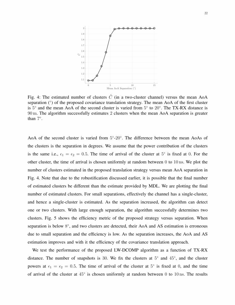
Fig. 4: The estimated number of clusters C (in a two-cluster channel) versus the mean AoAseparation (◦) of the proposed covariance translation strategy. The mean AoA of the first clusteris 5◦ and the mean AoA of the second cluster is varied from 5◦ to 20◦. The TX-RX distance is90 m. The algorithm successfully estimates 2 clusters when the mean AoA separation is greaterthan 7◦.

AoA of the second cluster is varied from 5◦-20◦. The difference between the mean AoAs of

the clusters is the separation in degrees. We assume that the power contribution of the clusters

is the same i.e., ε1 = ε2 = 0.5. The time of arrival of the cluster at 5◦ is fixed at 0. For the

other cluster, the time of arrival is chosen uniformly at random between 0 to 10 ns. We plot the

number of clusters estimated in the proposed translation strategy versus mean AoA separation in

Fig. 4. Note that due to the robustification discussed earlier, it is possible that the final number

of estimated clusters be different than the estimate provided by MDL. We are plotting the final

number of estimated clusters. For small separations, effectively the channel has a single-cluster,

and hence a single-cluster is estimated. As the separation increased, the algorithm can detect

one or two clusters. With large enough separation, the algorithm successfully determines two

clusters. Fig. 5 shows the efficiency metric of the proposed strategy versus separation. When

separation is below 8◦, and two clusters are detected, their AoA and AS estimation is erroneous

due to small separation and the efficiency is low. As the separation increases, the AoA and AS

estimation improves and with it the efficiency of the covariance translation approach.

We test the performance of the proposed LW-DCOMP algorithm as a function of TX-RX

distance. The number of snapshots is 30. We fix the clusters at 5◦ and 45◦, and the cluster

powers at ε1 = ε2 = 0.5. The time of arrival of the cluster at 5◦ is fixed at 0, and the time

of arrival of the cluster at 45◦ is chosen uniformly at random between 0 to 10 ns. The results

23

Fig. 5: The efficiency metric η (in a two-cluster channel) versus the mean AoA separation (◦)of the proposed covariance translation strategy. The mean AoA of the first cluster is 5◦ andthe mean AoA of the second cluster is varied from 5◦ to 20◦. The TX-RX distance is 90 m.The efficiency is high when the algorithm at low (high) mean AoA separations as the algorithmsuccessfully estimates 1 (2) clusters.

Fig. 6: The efficiency metric η (in a two-cluster channel) of the the proposed LW-DCOMPalgorithm versus the TX-RX distance (m). First cluster has mean AoA 5◦ and the second clusterhas a mean AoA 45◦. The number of snapshots T is 30. The out-of-band aided LW-DCOMPapproach performs better at large TX-RX distances.

of this experiment are shown in Fig. 6. We see that as the TX-RX separation increases - and

the SNR decreases - the benefit of using out-of-band information in compressed covariance

estimation becomes clear.

So far we did not consider the spatial discrepancy in the sub-6 GHz and mmWave channels. We

now test the performance of the proposed strategies in more realistic channels, i.e., where sub-6

24

GHz and mmWave systems have a mismatch. Specifically, we generate the channels according

to the methodology proposed in [26]. We refer the interested reader to [26] for the details

of the method to generate sub-6 GHz and mmWave channels. Here, we only give the channel

parameters. The sub-6 GHz and mmWave channels have C = 10 and C = 5 clusters respectively,

each contributing Rc = Rc = 20 rays. The mean angles of the clusters are limited to [−π3, π

3). The

relative angle shifts come from a wrapped Gaussian distribution with with AS {σϑc , σϕc} = 4◦

and {σϑc , σϕc} = 2◦ As the delay spread of sub-6 GHz channel is expected to be larger than the

delay spread of mmWave [48]–[51], we choose τRMS ≈ 3.8 ns and τRMS ≈ 2.7 ns. The relative

time delays of the paths within the clusters are drawn from zero mean Normal distributions

with RMS AS στrc=

τRMS

10and στrc = τRMS

10. The powers of the clusters are drawn from

exponential distributions. Specifically, the exponential distribution with parameter µ is defined as

f(x|µ) = 1µe−

xµ . The parameter for sub-6 GHz was chosen as µ = 0.2 and for mmWave µ = 0.1.

This implies that the power in late arriving multi-paths for mmWave will decline more rapidly

than sub-6 GHz. The system parameters are identical to the previously explained setup. The

hybrid precoders/combiners are designed using the greedy algorithm given in [3]. The effective

achievable rate results are shown in Fig. 7. For compressed covariance estimation and weighted

compressed covariance estimation, we assume that Tstat = 2048. The number of training OFDM

blocks is Ttrain = 2×2×T . Here, T is the number of snapshots. A factor of 2 appears as we use

2 OFDM blocks to create omnidirectional transmission, i.e., one snapshot. Another factor of 2

appears as the training is performed for the transmit and the receive covariance estimation. The

ideal case - i.e., sample covariance based on perfect channel knowledge - is also plotted. The

rate for the ideal case is calculated assuming no overhead. The observations about the benefit of

using out-of-band information in mmWave covariance estimation also hold in this experiment.

Note that, the achievable rate drops with increasing TX-RX distance due to decreasing SNR.

Further, this experiment validates the robustness of the designed covariance estimation strategies

to the correlated channel taps case.

We now compare the overhead of the proposed LW-DCOMP approach to the DCOMP ap-

proach. We use Ttrain = 2×2×T for rate calculations. In Fig. 8, we plot the effective achievable

rate versus the number of snapshots T for three different values of Tstat. For dynamic channels,

i.e., with Tstat = 1024 or Tstat = 2048, the effective rate of both LW-DCOMP and DCOMP

increases with snapshots, but as we keep on increasing T , the rate starts to decrease. This is

because, though the channel estimation quality increases, a significant fraction of the Tstat is

25

Fig. 7: The effective achievable rate of the proposed covariance estimation strategies versus theTX-RX distance. The rate calculations are based on Tstat = 2048 blocks and Ttrain = 120 blocks.The benefit of out-of-band information becomes more pronounced at high TX-RX distances.

Fig. 8: The effective achievable rate of LW-DCOMP and DCOMP versus the number of snapshotsT (at the transmitter and the receiver). The effective rate is plotted for three values of Tstat. TheTX-RX distance is fixed at 70 m. The LW-DCOMP reduces the training overhead of DCOMPby over 3x.

spent training and the thus there is less time to use the channel for data transmission. Taking

Tstat = 2048 as an example, the highest rate of DCOMP algorithm is 7.16 b/s/Hz and is

achieved with 45 snapshots. In comparison, the optimal rate of the LW-DCOMP algorithm is

7.46 b/s/Hz and is achieved with only 25 snapshots. The LW-DCOMP achieves a rate better

than the highest rate of DCOMP algorithm (7.16 b/s/Hz) with less than 15 snapshots. Thus,

the LW-DCOMP can reduce the training overhead of DCOMP by over 3x.

Now we verify the SNR loss analysis outlined in Section V. For this purpose, we consider

26

Fig. 9: The upper bound on the SNR loss γ with complex Normal perturbation. The number ofRF-chains is MTX = MRX =

√NTX =

√NRX and SNRk = P

σ2nK

. The upper-bound derived inthe analysis holds for both the tested scenarios.

two mmWave systems with NTX = NRX = 64 and NTX = NRX = 16 antennas. The number of

RF-chains in both cases is MTX = MRX =√NTX =

√NRX. We plot the loss in SNR γ as a

function of the SNR per-subcarrier i.e., SNRk = Pσ2nK

. We assume that [∆RRX]i,j = [∆RTX]i,j ∼

CN (0, 1SNRk

). The smallest singular value of the Gaussian matrices vanishes as the dimensions

increase [52], and the analytical lower bound (33) becomes trivial. As such, we only show the

analytical upper bound (32) in Fig. 9. We compare the upper bound on SNR loss (32) and

the empirical difference in the average SNR of the mmWave systems based on true covariance

and the perturbed covariance. The empirical difference is plotted for the case when the singular

vectors are used as precoder/combiner (i.e., assuming fully digital precoding/combining) and

also for the case when hybrid precoders/combiners are used. From the results, we can see that

the upper bound is valid for both systems with 16 and 64 antennas respectively. An interesting

observation is that when the hybrid precoders/combiners are used in the mmWave system, the

loss due to the mismatch in the estimated and true covariance is less than the case when fully

digital precoding and combining is used.

VII. COMPARISON OF PROPOSED COVARIANCE ESTIMATION STRATEGIES

We now compare some characteristics of the proposed covariance estimation strategies.

27

A. Computational complexity

The out-of-band covariance translation has four steps. The computational complexity of the

first two steps at the receiver is dictated by the eigenvalue decomposition of the covariance matrix,

i.e., O(N3RX). The computational complexity of finding the cluster powers using least-squares

(i.e., the third step) is O(C2N2RX). Finally, the computational complexity of fourth step, i.e.,

constructing the mmWave covariance, is O(CN2RX). For the out-of-band aided compressed co-

variance estimation strategy, the online computational complexity of the LW-DCOMP algorithm

is O(TBRXM2RXL).

B. Overhead

The out-of-band covariance translation completely eliminates the in-band training. As the

sub-6 GHz channel information is required for the operation of sub-6 GHz system, the out-of-

band covariance translation does not have a training overhead. The out-of-band aided compressed

covariance estimation strategy uses in-band training in conjunction with out-of-band information.

The in-band training overhead, however, is very small. As shown in Fig. 8, the proposed out-of-

band aided compressed covariance estimation has an achievable rate of more than 7 (b/s/Hz)

with only 5 snapshots.

C. Robustness to erroneous information

The out-of-band covariance translation relies completely on sub-6 GHz information. As such,

the out-of-band covariance translation may perform poorly if the mmWave and sub-6 GHz chan-

nels are spatially incongruent. The out-of-band aided compressed covariance estimation relies

on in-band as well as out-of-band information. The reliance on in-band information makes it

more robust to spatial incongruence between sub-6 GHz and mmWave channels.

D. Inherent limitations

The out-of-band covariance translation is based on parametric estimation. The number of

point sources that can be estimated at the receiver are NRX − 1. This translates to C =

max{bNRX−1

2c, 1} estimated clusters. As such, the translated mmWave covariance is also limited

to C clusters. The out-of-band aided compressed covariance strategy assumes limited scattering

of the mmWave channel. Further, the covariance recovery is limited by the number of RF-chains

28

in the mmWave system. Specifically, it is required that the number of coefficients with significant

magnitude be L ≤MRX.

E. Favorable operating conditions

If the TX-RX separation is small, i.e., the SNR is high, the out-of-band aided compressed

covariance estimation performs better than out-of-band covariance translation (see Fig. 8). As

the TX-RX distance increases, however, the out-of-band covariance translation starts to perform

better. This result informs that depending on the TX-RX separation (or the SNR), the out-of-

band aided compressed covariance estimation or the out-of-band covariance translation may be

preferred.

VIII. CONCLUSION

In this paper, we used the sub-6 GHz covariance to predict the mmWave covariance. We

presented a parametric approach that relies on the estimates of mean angle and angle spread

and their subsequent use in theoretical expressions of the covariance pertaining to a postulated

power azimuth spectrum. To aid the in-band compressed covariance estimation with out-of-

band information, we formulated the compressed covariance estimation problem as weighted

compressed covariance estimation. For a single path channel, we bounded the loss in SNR caused

by imperfect covariance estimation using singular-vector perturbation theory.

The out-of-band covariance translation and out-of-band aided compressed covariance estima-

tion had better effective achievable rate than in-band only training, especially in low SNR scenar-

ios. The out-of-band covariance translation eliminated the in-band training but performed poorly

(in comparison with in-band training) when the SNR of the mmWave link was favorable. The

out-of-band aided compressed covariance estimation reduced the training overhead of the in-band

only covariance estimation by 3x. The benefit of the proposed strategies was more pronounced

in highly dynamic channels, making the strategies suitable for V2X communication. As a future

work, covariance estimation approaches for array geometries other than uniform linear arrays,

e.g., circular and planar arrays should be explored.

APPENDIX A

29

PROOF OF THEOREM 1

The received signal (28) can be written as

y =u∗RX,sHuTX,s

‖uRX,s‖‖uTX,s‖s +

∆u∗RX,sHuTX,s

‖uRX,s‖‖uTX,s‖s

+u∗RX,sH∆uTX,s

‖uRX,s‖‖uTX,s‖s +

∆u∗RX,sH∆uTX,s

‖uRX,s‖‖uTX,s‖s +

u∗RX,s

‖uRX,s‖n. (36)

The numerator of the first term on the RHS is identical to the first term in (24) and can be

simplified as

u∗RX,sHuTX,s

‖uRX,s‖‖uTX,s‖s =

√NRXNTXαs

‖uRX,s‖‖uTX,s‖. (37)

Now using the channel representation in form of the signal subspace H =√NRXNTXαuRX,su

∗TX,s,

the second term can be written as

∆u∗RX,sHuTX,s

‖uRX,s‖‖uTX,s‖s =

√NRXNTXα∆u∗RX,suRX,su

∗TX,suTX,s

‖uRX,s‖‖uTX,s‖s. (38)

Using the results from [13] we can write ∆uRX,s as

∆uRX,s =URX,nU

∗RX,n∆RRXuRX,s

σ2αNRX

, (39)

and further

∆u∗RX,suRX,s =u∗RX,s∆R∗RXURX,nU

∗RX,nuRX,s

σ2αNRX

. (40)

In (40), U∗RX,nuRX,s = 0, and hence the second term in (36) is zero. The third term and the fourth

term in (36) vanish by the same argument. Hence the received signal can be simply written as

y =

√NRXNTXαs

‖uRX,s‖‖uTX,s‖+

u∗RX,s

‖uRX,s‖n, (41)

from which SNR expression (29) can be obtained.

APPENDIX B

30

PROOF OF THEOREM 2

We work solely on simplifying uRX,s on the RHS of (30) as the simplification of uTX,s is

analogous. We can write

‖uRX,s‖2 (a)= ‖uRX,s + ∆uRX,s‖2 (b)

= ‖uRX,s‖2 + ‖∆uRX,s‖2,

(c)= 1 +

1

σ4αN

2RX

∥∥URX,nU∗RX,n∆RRXuRX,s

∥∥2,

(d)≈ 1 +

1

σ4αN

2RX

‖∆RRXuRX,s‖2 , (42)

where (a) comes from the definition of uRX,s and (b) comes from the assumption that the

phase of the perturbation is adjusted to have the true signal subspace and the perturbation signal

subspace orthogonal [13]. In (c) the first term simplifies to 1 as the norm of the singular vector

and the second term comes from the definition of ∆uRX,s in (39). Finally in (d) we use the

approximation URX,nU∗RX,n ≈ I. Note that for a single path channel, the channel subspace is

one dimensional and‖URX,nU

∗RX,n−INRX

‖2F‖INRX

‖2F= 1

NRX. Hence

‖URX,nU∗RX,n−INRX

‖2F‖INRX

‖2F→ 0 as NRX →∞

and the approximation is exact in the limit. For mmWave systems where the number of antennas

is typically large, the approximation is fair. Following an analogous derivation for uTX,s, we

get (31).

To obtain the upper and lower bounds, note the following about the norm of a matrix-vector

product Ax: max‖x‖2=1 ‖Ax‖2 = σ2max(A) and min‖x‖2=1 ‖Ax‖2 = σ2

min(A), where σmax(A)

and σmin(A) is the largest and smallest singular value of the matrix A. As in (31), uRX,s is a

singular vector with unit norm, we can bound σmin(∆RRX) ≤ ‖∆RRXuRX,s‖ ≤ σmax(∆RRX).

Using this result in (31), we get (32) and (33).

REFERENCES

[1] A. Ali, N. Gonzalez-Prelcic, and R. W. Heath Jr., “Estimating millimeter wave channels using out-of-band measurements,”

in Proc. Inf. Theory Appl. (ITA) Wksp, Feb. 2016, pp. 1–6.

[2] O. El Ayach et al., “Spatially sparse precoding in millimeter wave MIMO systems,” IEEE Trans. Wireless Commun.,

vol. 13, no. 3, pp. 1499–1513, Mar. 2014.

[3] A. Alkhateeb et al., “Hybrid precoding for millimeter wave cellular systems with partial channel knowledge,” in Proc. Inf.

Theory Appl. (ITA) Wksp, Feb. 2013, pp. 1–5.

[4] J. Mo and R. W. Heath Jr., “Capacity analysis of one-bit quantized MIMO systems with transmitter channel state

information,” IEEE Trans. Signal Process., vol. 63, no. 20, pp. 5498–5512, 2015.

[5] Y. Kishiyama et al., “Future steps of LTE-A: Evolution toward integration of local area and wide area systems,” IEEE

Wireless Commun., vol. 20, no. 1, pp. 12–18, Feb. 2013.

31

[6] R. C. Daniels and R. W. Heath Jr., “Multi-band modulation, coding, and medium access control,” IEEE 802.11-07/2780R1,

pp. 1–18, Nov. 2007.

[7] M. Hashemi, C. E. Koksal, and N. B. Shroff, “Out-of-band millimeter wave beamforming and communications to achieve

low latency and high energy efficiency in 5G systems,” IEEE Trans. Commun., vol. 66, no. 2, pp. 875–888, 2018.

[8] Z. Pi and F. Khan, “An introduction to millimeter-wave mobile broadband systems,” IEEE Commun. Mag., vol. 49, no. 6,

pp. 101–107, Jun. 2011.

[9] T. Bai and R. W. Heath Jr., “Coverage and rate analysis for millimeter-wave cellular networks,” IEEE Trans. Wireless

Commun., vol. 14, no. 2, pp. 1100–1114, Feb. 2015.

[10] J. Choi et al., “Millimeter wave vehicular communication to support massive automotive sensing,” IEEE Commun. Mag.,

vol. 54, no. 12, pp. 160–167, Dec. 2016.

[11] Y. J. Li, “An overview of the DSRC/WAVE technology,” in Proc. Qual., Rel., Security Robustness Heterogeneous Netw.

Springer, Nov. 2010, pp. 544–558.

[12] J. Scarlett, J. S. Evans, and S. Dey, “Compressed sensing with prior information: Information-theoretic limits and practical

decoders,” IEEE Trans. Signal Process., vol. 61, no. 2, pp. 427–439, Jan 2013.

[13] J. Liu, X. Liu, and X. Ma, “First-order perturbation analysis of singular vectors in singular value decomposition,” IEEE

Trans. Signal Process., vol. 56, no. 7, pp. 3044–3049, 2008.

[14] M. D. Larsen and A. L. Swindlehurst, “A MIMO channel perturbation analysis for robust bit loading,” in Proc. IEEE Int.

Conf. Acoust., Speech Signal Process. (ICASSP), Apr. 2009, pp. 2825–2828.

[15] J. Zhang, M. Haardt, and F. Roemer, “Robust design of block diagonalization using perturbation analysis,” in Proc. IEEE

Int. Conf. Acoust., Speech Signal Process. (ICASSP), May 2013, pp. 4192–4196.

[16] B. K. Chalise, L. Haering, and A. Czylwik, “Robust uplink to downlink spatial covariance matrix transformation for

downlink beamforming,” in Proc. IEEE Int. Conf. Commun. (ICC), vol. 5, Jun. 2004, pp. 3010–3014.

[17] K. Hugl, J. Laurila, and E. Bonek, “Downlink beamforming for frequency division duplex systems,” in Proc. IEEE Glob.

Telecom. Conf. (GLOBECOM), vol. 4, Dec. 1999, pp. 2097–2101.

[18] M. Jordan, X. Gong, and G. Ascheid, “Conversion of the spatio-temporal correlation from uplink to downlink in FDD

systems,” in Proc. IEEE Wireless Commun. Netw. Conf. (WCNC), Apr. 2009, pp. 1–6.

[19] A. Decurninge, M. Guillaud, and D. T. Slock, “Channel covariance estimation in massive MIMO frequency division duplex

systems,” in Proc. IEEE Glob. Telecom. Conf. (GLOBECOM), Dec. 2015, pp. 1–6.

[20] L. Miretti, R. L. Cavalcante, and S. Stanczak, “FDD massive MIMO channel spatial covariance conversion using projection

methods,” arXiv preprint arXiv:1804.04850, 2018.

[21] D. Vasisht et al., “Eliminating channel feedback in next-generation cellular networks,” in Proc. ACM SIGCOMM, Aug.

2016, pp. 398–411.

[22] J. Shen et al., “Compressed CSI acquisition in FDD massive MIMO: How much training is needed?” IEEE Trans. Wireless

Commun., vol. 15, no. 6, pp. 4145–4156, Jun. 2016.

[23] K. Hugl, K. Kalliola, and J. Laurila, “Spatial reciprocity of uplink and downlink radio channels in FDD systems,” May

2002, COST 273 Technical Document TD(02) 066.

[24] V. Raghavan et al., “Low-frequency assisted methods for beamforming, timing and frequency offset in mm-wave access

systems,” May 2016, US Patent 9,337,969. [Online]. Available: https://www.google.com/patents/US9337969

[25] T. Nitsche et al., “Steering with eyes closed: mm-wave beam steering without in-band measurement,” in Proc. IEEE Int.

Conf. Comput. Commun. (INFOCOM), Apr. 2015, pp. 2416–2424.

[26] A. Ali, N. Gonzalez-Prelcic, and R. W. Heath Jr., “Millimeter wave beam-selection using out-of-band spatial information,”

IEEE Trans. Wireless Commun., vol. 17, no. 2, pp. 1038–1052, 2018.

32

[27] N. Gonzalez-Prelcic, R. Mendez-Rial, and R. W. Heath Jr., “Radar aided beam alignment in mmwave V2I communications

supporting antenna diversity,” in Proc. Inf. Theory Appl. (ITA) Wksp, Feb. 2016, pp. 1–5.

[28] R. Mendez-Rial, N. Gonzalez-Prelcic, and R. W. Heath Jr., “Adaptive hybrid precoding and combining in mmWave

multiuser MIMO systems based on compressed covariance estimation,” in Proc. IEEE Int. Workshop Comput. Adv. Multi-

Sensor Adapt. Process. (CAMSAP), Dec. 2015, pp. 213–216.

[29] S. Park and R. W. Heath Jr., “Spatial channel covariance estimation for mmWave hybrid MIMO architecture,” in Proc.

Asilomar Conf. Signals, Syst. Comput. (ASILOMAR), Nov. 2016, pp. 1424–1428.

[30] S. Park and R. W. Heath Jr, “Spatial Channel Covariance Estimation for the Hybrid MIMO Architecture: A Compressive

Sensing Based Approach,” IEEE Trans. Wireless Commun., vol. 17, no. 12, pp. 8047–8062, 2018.

[31] H. Ji et al., “Overview of full-dimension MIMO in LTE-advanced pro,” IEEE Commun. Mag., vol. 55, no. 2, pp. 176–184,

2017.

[32] A. Alkhateeb and R. W. Heath Jr., “Frequency selective hybrid precoding for limited feedback millimeter wave systems,”

IEEE Trans. Commun., vol. 64, no. 5, pp. 1801–1818, May 2016.

[33] E. Bjornson, D. Hammarwall, and B. Ottersten, “Exploiting quantized channel norm feedback through conditional statistics

in arbitrarily correlated MIMO systems,” IEEE Trans. Signal Process., vol. 57, no. 10, pp. 4027–4041, 2009.

[34] N. Czink et al., “Improved MMSE estimation of correlated MIMO channels using a structured correlation estimator,” in

Proc. IEEE Int. Workshop Signal Process. Adv. Wireless Commun. (SPAWC), Jun. 2005, pp. 595–599.

[35] M. Bengtsson and B. Ottersten, “Low-complexity estimators for distributed sources,” IEEE Trans. Signal Process., vol. 48,

no. 8, pp. 2185–2194, Aug. 2000.

[36] A. Forenza, D. J. Love, and R. W. Heath Jr., “Simplified spatial correlation models for clustered MIMO channels with

different array configurations,” IEEE Trans. Veh. Technol., vol. 56, no. 4, pp. 1924–1934, Jul. 2007.

[37] M. Wax and T. Kailath, “Detection of signals by information theoretic criteria,” IEEE Trans. Acoust., Speech, Signal

Process., vol. 33, no. 2, pp. 387–392, Apr. 1985.

[38] H. Akaike, “A new look at the statistical model identification,” IEEE Trans. Autom. Control, vol. 19, no. 6, pp. 716–723,

Dec. 1974.

[39] A. J. Barabell, “Improving the resolution performance of eigenstructure-based direction-finding algorithms,” in Proc. IEEE

Int. Conf. Acoust., Speech Signal Process. (ICASSP), vol. 8, Apr. 1983, pp. 336–339.

[40] D. Romero et al., “Compressive covariance sensing: Structure-based compressive sensing beyond sparsity,” IEEE Signal

Process. Mag., vol. 33, no. 1, pp. 78–93, 2016.

[41] J. M. Bioucas-Dias, D. Cohen, and Y. C. Eldar, “Covalsa: Covariance estimation from compressive measurements using

alternating minimization,” in Proc. Eur. Signal Process. Conf. (EUSIPCO), Sep. 2014, pp. 999–1003.

[42] J. Rodriguez-Fernandez, R. Lopez-Valcarce, and N. Gonzalez-Prelcic, “Hybrid precoding and combining for frequency-

selective mmWave MIMO Systems with per-antenna power constraints,” arXiv preprint arXiv:1812.02760, 2018.

[43] A. Alkhateeb et al., “Channel estimation and hybrid precoding for millimeter wave cellular systems,” IEEE J. Sel. Topics

Signal Process., vol. 8, no. 5, pp. 831–846, Oct. 2014.

[44] A. M. Sayeed, “Deconstructing multiantenna fading channels,” IEEE Trans. Signal Process., vol. 50, no. 10, pp. 2563–2579,

Oct. 2002.

[45] S. Haghighatshoar and G. Caire, “Massive MIMO channel subspace estimation from low-dimensional projections,” IEEE

Trans. Signal Process., vol. 65, no. 2, pp. 303–318, 2017.

[46] F. C. Commission et al., “Amendment of the commissions rules with regard to commercial operations in the 3550-3650

MHz band,” GN Docket, no. 12-354, 2012.

33

[47] ——, “Fact sheet: spectrum frontiers rules identify, open up vast amounts of new high-band spectrum for next generation

(5G) wireless broadband,” 2016. [Online]. Available: https://apps.fcc.gov/edocs\ public/attachmatch/DOC-340310A1.pdf

[48] R. J. Weiler et al., “Simultaneous millimeter-wave multi-band channel sounding in an urban access scenario,” in Proc.

Eur. Conf. Antennas Propag. (EuCAP), Apr. 2015, pp. 1–5.

[49] A. S. Poon and M. Ho, “Indoor multiple-antenna channel characterization from 2 to 8 GHz,” in Proc. IEEE Int. Conf.

Commun. (ICC), May 2003, pp. 3519–3523.

[50] S. Jaeckel et al., “5G channel models in mm-wave frequency bands,” in Proc. Eur. Wireless Conf. (EW), May 2016, pp.

1–6.

[51] A. O. Kaya, D. Calin, and H. Viswanathan. (2016, Apr.) 28 GHz and 3.5 GHz wireless channels: Fading, delay and angular

dispersion.

[52] R. Vershynin, “Introduction to the non-asymptotic analysis of random matrices,” arXiv preprint arXiv:1011.3027, 2010.


Recommended