Spatial Econometric Modelsof Interdependence

Theory & Substance; Empirical Specification, Estimation, Evaluation; Substantive

Interpretation & Presentation

Talk prepared for Blalock Lecture on7 August 2008 at the ICPSR Summer School

based on the joint work ofRobert J. Franzese, Jr., The University of Michigan

Jude C. Hays, The University of Illinois

• Motivation: Integration & Domestic Policy-Autonomy– Does economic integration constrain govts from redistributing

income, risk, & opportunity through tax & spending policies?– In answering this & related questions, scholars have overlooked

spatial interdependence of domestic policies as important evidence.

– Economic integration generates externalities across political jurisdictions, which implies strategic policy interdependence, so policy of one govt will be influenced by policies of its neighbors.

• Interdependence Substance, Theory, & Empirics: Use contexts econ integration (& related) to explore & explain:– Substance: i’s actions depend on j’s. Examples.– Theory:

• General: externalitiesstrategic policy complements/substitutesrace-to-bottom/top/elseearly/late-mover advantagesstrategic delay/rush-for-1st

• Specific: a model of inter-jurisdictional tax-competition (P&T ch. 12)– Empirics: “Galton’s Problem”; Estimation, Inference,

Interpretation, & Presentation

Overview

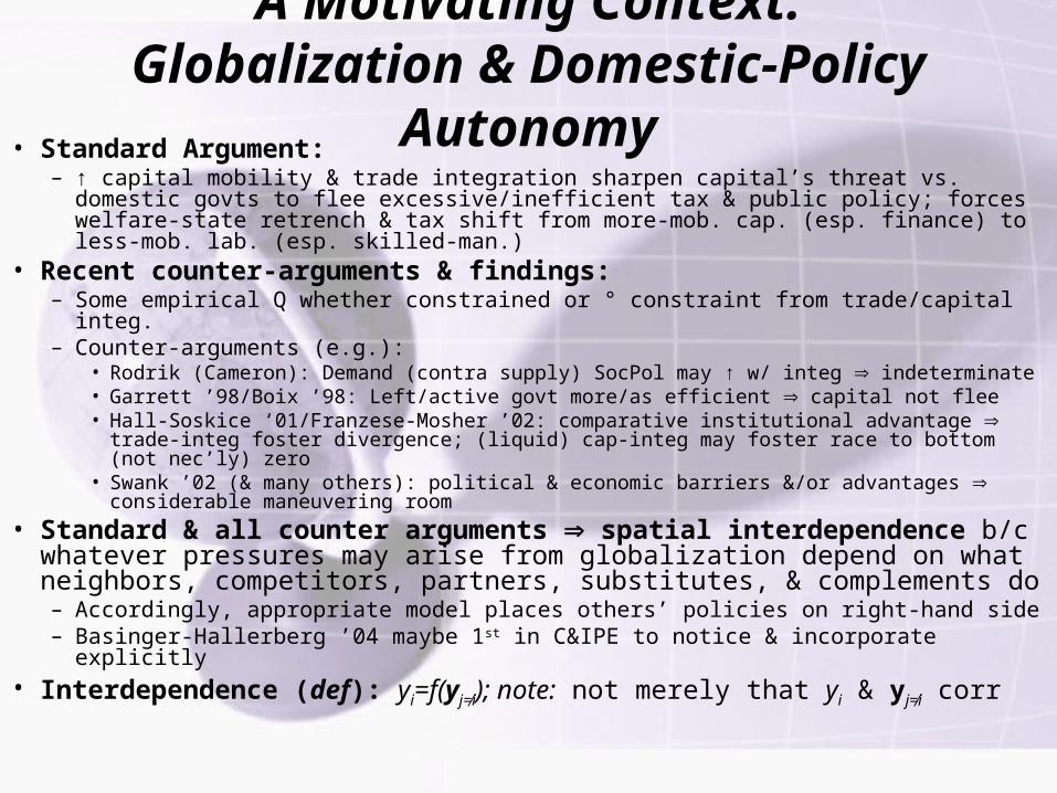
• Standard Argument:– ↑ capital mobility & trade integration sharpen capital’s threat vs. domestic govts

to flee excessive/inefficient tax & public policy; forces welfare-state retrench & tax shift from more-mob. cap. (esp. finance) to less-mob. lab. (esp. skilled-man.)

• Recent counter-arguments & findings:– Some empirical Q whether constrained or ° constraint from trade/capital integ.– Counter-arguments (e.g.):

• Rodrik (Cameron): Demand (contra supply) SocPol may ↑ w/ integ indeterminate• Garrett ’98/Boix ’98: Left/active govt more/as efficient capital not flee• Hall-Soskice ‘01/Franzese-Mosher ’02: comparative institutional advantage trade-

integ foster divergence; (liquid) cap-integ may foster race to bottom (not nec’ly) zero• Swank ’02 (& many others): political & economic barriers &/or advantages

considerable maneuvering room

• Standard & all counter arguments spatial interdependence b/c whatever pressures may arise from globalization depend on what neighbors, competitors, partners, substitutes, & complements do– Accordingly, appropriate model places others’ policies on right-hand side– Basinger-Hallerberg ’04 maybe 1st in C&IPE to notice & incorporate explicitly

• Interdependence (def): yi=f(yj≠i); note: not merely that yi & yj≠i corr

A Motivating Context:Globalization & Domestic-Policy Autonomy

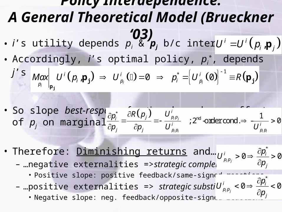
• Theoretical Contexts (ubiquitous):– ANY Strategic Decision-making: sisj

– Externalities & Spillovers– Learning/Emulation, Demonstration– Networks/Epistemic Communities– Literal Diffusion, Contagion, Migration

The Broad Range of Spatial Interdependence

• Tobler’s Law: ‘‘I invoke the first law of geography: everything is related to everything else, but near things are more related than distant things’’ (1970).– Plus: “Space More Than Geography” (Beck, Gleditsch, & Beardsley 2006)

• Substantive Contexts (ubiquitous):– Security Policy (e.g., alliances, wars)

– Environmental (e.g., air-pollution reg)

– Regulatory (e.g., telecomm stds)

– Legis reps’ votes depend on others’

– Elects., cand. qualities or strategies– p(∙)&outs coups (Li&Thompson 75), riots

(Govea&West 81), revolts (Brinks&Copp 06)

– Contextual effects in micro-behavior:• Braybeck&Huckfeldt 02ab, Cho 03, Huckfeldt et al.

05, Cho&Gimpel 07, Cho&Rudolph 07, Lin et al 06

• (Simmons et al.’s 06) Mechanisms:– Competition– Coercion– Learning– Emulation– [Migration/Contagion (F&H Add)]

– Policy, instit’s, regimes diffusion:• Policy: Schneider&Ingram‘88, Rose ‘93,

Meseguer ‘04,‘05, Gilardi ‘05

• Institutional or regime: Implicit/Informal: Dahl’s Polyarchy, Starr’s Democratic Dominoes, Huntington’s 3rd Wave. Explicit/Formal: O’Loughlin et al. ‘98, Brinks & Coppedge ‘06, Gleditsch & Ward ‘06, ’07

– Int’l diffusion of liberalization:• Simmons&Elkins 04, 06a, 06b, Eising 02,

Brune et al. 04, Brooks 05…

– Globalization & interdependence:• Genschel 02, Basinger&Hallerberg 04, Knill

05, Jahn 06, Swank 06, F&H 06,07, Kayser 07

Substantive & Theoretical Ubiquity & Centrality (1)

•US State Policy-innovation diffusion: deep roots & much contemporary interest, & sustained attention between:

– Crain 1966; Walker 1969, 1973; Gray 1973; Knoke 1982; Caldiera 1985; Lutz 1987; Berry & Berry 1990; Case et al. 1993; Berry 1994; Rogers 1995; Mintrom 1997ab; Brueckner 1998; Mintrom & Vergari 1998; Mossberger 1999; Berry & Berry 1999; Godwin & Schroedel 2000; Balla 2001; Mooney 2001; Wejnert 2002; Coughlin et al. 2003; Bailey & Rom 2004; Boehmke & Witmer 2004; Daley & Garand 2004; Grossback et al. 2004; Mencken 2004; Berry & Baybeck 2005; Garrett et al. 2005; Costa-Font & Ons-Novell 2006; Karch 2006; Rincke 2006; Shipan & Volden 2006; Volden 2006; Werck et al. 2006; Woods 2006; Volden et al. 2007.

•Similar policy-learning mechanisms underlie some comparative studies of policy diffusion:

– Schneider & Ingram 1988; Rose 1993; Bennett 1997; Dolowitz & Marsh 2000; True & Mintrom 2001; Tews et al. 2003; Jensen 2004; Meseguer 2004, 2005; Brooks 2005, 2007; Gilardi 2005; Gilardi et al. 2005; Murillo & Schrank 2005; Weyland 2005; Braun & Gilardi 2006; Linos 2006; Parys 2006; Ermini & Santolini 2007; Moscone et al. 2007.

•Institutional or regime diffusion likewise long-standing & recently much reinvigorated:

– Dahl’s 1971 Polyarchy (1 of 8 causes dem listed); center-stage Starr’s 1991 “Democratic Dominoes”; Huntington’s 1991 Third Wave; Beissinger 2007; Bunce & Wolchik 2006, 2007; et al. in E. Eur. Transitions; Hagopian & Mainwaring 2005 et al. in LA; O’Loughlin et al. 1998, Brinks & Coppedge 2006, Gleditsch & Ward 2006, 2007 estimated empirically extent, paths, &/or patterns dem diffuse. Kelejian et al. 2007 give institutional diffusion general theoretical & empirical treatment.

•C&IPE, e.g. globalization≈interdependence:– Diffusion of “Liberalization” & Related: Simmons & Elkins 2004, Simmons et al. 2006,

Eising 2002; Brune et al. 2004; Brooks 2005, 2007; Jordana & Levi-Faur 2005; Way 2005; Lazer 2006; Prakash & Potoski 2006; Brune & Guisinger 2007; and many others.

– Glob/Interdep/TaxComp & Dom Policy Auton: Genschel 2002; Guler et al. 2002; Franzese & Hays 2003, 2004b, 2005a, 2007abc, 2008c; Badinger et al. 2004; Basinger & Hallerberg 2004; Heichel et al. 2005; Henisz et al. 2005; Holzinger & Knill 2005; Knill 2005; Polillo & Guillén 2005; Elkins et al. 2006; Jahn 2006; Lee & Strang 2006; Manger 2006; Swank 2006; Baturo & Grey 2007; Cao 2007; Cao et al. 2007; Coughlin et al. 2007; Garretsen & Peeters 2007; Mosley & Uno 2007; Mukherjee & Singer 2007.

Substantive & Theoretical Ubiquity & Centrality (2)• Representatives’ votes (Lacombe & Shaughnessy 2005), citizens’ votes (Huckfeldt & Sprague 1991;

O’Laughlin et al. 1994; Pattie & Johnston 2000; Beck et al. 2003; Calvo & Escolar 2003; Kim et al. 2003; Schofield et al. 2003; Lacombe &

Shaughnessy 2007), election outcomes (Shin & Agnew 2002, 2007; Hiskey & Canache 2005; Wing & Walker 2006;

Kayser 2007), candidate qualities, contributions, or strategies (Goldenberg et al. 1986; Mizruchi 1989; Krasno et al. 1994; Cho 2003; Gimpel et al. 2006)

• Probabilities & outcomes of coups (Li & Thompson 1975), riots (Govea & West 1981), civil wars (Murdoch & Sandler 2004, Buhaug & Rød 2006) &/or revolutions (Brinks & Coppedge 2006)

• IR: interdep≈definition of subject: – States’ entry into wars, alliances, treaties (Murdoch et al. 2003), or

organizations.– Empirical attention to inherent spat-dep IR greatest in: Shin & Ward 1999;

Gleditsch & Ward 2000; Gleditsch 2002; Ward & Gleditsch 2002; Hoff & Ward 2004; Gartzke & Gleditsch 2006; Salehyan & Gleditsch

2006; Gleditsch 2007, and, in different way, Signorino 1999, 2002, 2003; Signorino & Yilmaz 2003; Signorino & Tarar 2006

• In micro-behavioral work, too, long-standing & surging interest “contextual” or “neighborhood” effects:

– Huckfeldt & Sprague 1993 review, some of which stress interdep: Straits 1990; O’Loughlin et al. 1994; Knack & Kropf 1998; Liu et al. 1998; Braybeck & Huckfeldt 2002ab; Beck et al. 2002; McClurg 2003; Huckfeldt et al. 2005; Cho & Gimpel 2007; Cho & Rudolph 2007. Sampson et al. 2002 and Dietz 2002 review the parallel large literature on neighborhood effects in sociology

• At & beyond other disciplinary borders, subjects include:– Social-movements: McAdam & Rucht 1993; Conell & Cohn 1995; Giugni 1998; Strang & Soule 1998; Biggs 2003;

Browning et al. 2004; Andrews & Biggs 2006; Holmes 2006; Swaroop & Morenoff 2006.

– Microeconomic preferences: Akerloff 1997; Postlewaite 1998; Glaeser & Scheinkman 2000; Manski 2000; Brock & Durlauf 2001; Durlauf 2001; Glaeser et al. 2003; Yang & Allenby 2003; Sobel 2005; Ioannides 2006; Soetevent 2006

– Macroeconomic performance: Fingleton 2003; Novo 2003; Kosfeld & Lauridsen 2004; Maza & Villaverde 2004; Kelejian et al. 2006; Mencken et al. 2006

– Technology, marketing, and other firm strategies: Abramson & Rosenkopf 1993; Geroski 2000; Strang & Macy 2001; Holloway 2002; Bradlow 2005; Autant-Berard 2006; Mizruchi et al. 2006

– Violence and crime: Grattet et al. 1998; Myers 2000; Baller et al. 2001; Morenoff et al. 2001; Villareal 2002; Baker & Faulkner 2003; Oberwittler 2004; Bhati 2005; Mears & Bhati 2006; Brathwaite & Li 2008

– Fertility, birthweight, child development, & child poverty: Tolnay 1995 and Montgomery & Casterline 1996; Morenoff 2003; Sampson et al. 1999; Voss et al. 2006

– Not to mention public health and epidemiology (contagion!).• More exotic topics: ordainment of women (Chaves 1996), right-wing

extremism (Rydgren 2005), marriage (Yabiku 2006), national identity (Lin et al. 2006), & faculty (Weinstein 2007).

• i’s utility depends pi & pj b/c interdep (& vv):

• Accordingly, i’s optimal policy, pi*, depends j’s action, pj:

• So slope best-response function depends on effect of pj on marginal utility of pi:

• Therefore: Diminishing returns and…– …negative externalities =>strategic complements:

• Positive slope: positive feedback/same-signed reactions

– …positive externalities => strategic substitutes:• Negative slope: neg. feedback/opposite-signed reactions

Policy Interdependence:A General Theoretical Model (Brueckner ‘03)

,i ii jU U p p

1*, 0 0i i

i

i i ii p i p

pMax U p U p U R

j

j jp

p p

*nd 1

; 2 -order cond. - 0i j

i i i i

ip pjii i

j j p p p p

UR pp

p p U U

*

0 0i j

i ip p

j

pU

p

*

0 0i j

i ip p

j

pU

p

Policy Interdependence:General Theory & Substantive Implications

• Dimin returns & neg externalities Strategic Complements Race-to-Bottom (RTB) (or -Top). Examples:

• Tax Competition• Labor Regulation• Trade Barriers (politically)

Early-mover advantage “race to go first”• E.g.: Exch.Deprec., tech.stds. (& other focal pts. in coord. or battle sexes)

• Dimin returns & pos externalities Strategic Substitutes– Free-Riding Incentives

• E.g., Alliance Security:• E.g., ALMP:

Late-mover advantage strategic delay & Wars of Attrition

• DimRet & both +&– externs:– Environmental Reg’s (& CHIPs?):

( marg cost ) i j

ij i iU

(b/c security ) i j

ij i iS U S

(b/c Emp ) i j

ij A A i iALMP U ALMP

environ j i iR R (Free - Ride)

cost j i iR R R (RTB)

Figure 2. Best Response Functions: Strategic Substitutes

)( 12 pRp

)( 21 pRp

•p2

•p1

Figure 1. Best Response Functions (Persson and Tabellini 2000, 334)

An International Tax-Competition Model as a Specific Substantive Example of Interdependence

• Stylized Theoretical Model Cap-Tax Comp. (P&T ‘00, ch.12)– 2 jurisdicts, dom & for cap-tax, τk & τk

* to fund fixed spend. For-invest mobility costs, M.– Inds’ lab-cap endow, ei, & choose lab-leisure, l & x, & save-invest, s=k+f to max

ω=U(c1)+c2+V(x), over l, c1, & c2, s.t. time-c., 1+ei=l+x, & b.c.’s, 1–ei=c1+k+f+≡c1+s & c2=(1–τk)k+(1–τk

*)f–M(f)+(1–τl)l. equilibrium economic choices of citizens:

indirect utility, W, defined over policy variables, τl, τk, & τk*:

– Besley-Coate (‘97) citizen-candidate(s) face(s) electorate w/ these prefs.• Stages: 1) elects, 2) cit-cand winners set taxes, 3) all private econ decisions made.• Ebm win cand has endow eP such that desires implement this Modified Ramsey Rule:

Best-Response Functions: τk=T(eP,τk*) & τk

*=T*(eP*,τk) for dom & for pm.– Slopes: ∂T/∂τk

* & ∂T*/∂τk, pos or neg b/c ↑τk* cap-inflow; can use ↑tax-base to ↓τk or to ↑τk

(seizing upon ↓elasticity base).– Background of this slide plots case both positively sloped; illustrated comparative static is

of leftward shift of domestic government.

1( ) 1 (1 )k c ks S U * 1 *( , ) ( )k k f k kf F M * *( , ) ( ) ( , )k k k k kk K S F

* * *( , ) 1 ( ) 1 ( ) ( , ) ( , ) 1 ( ) 1 ( )l k k k k k k k k k k l l lW U S S F M F L V L

* *( ) ( ) ( ) 2 ( , )1 ( ) 1

( ) ( ) ( )

p p p p p p ppk l k k k k

l kp p pk l k

S e L e S F

S L S

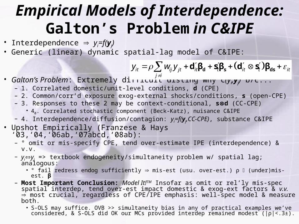
Empirical Models of Interdependence:Galton’s Problem in C&IPE

• Interdependence yi=f(yj)• Generic (linear) dynamic spatial-lag model of C&IPE:

• Galton’s Problem: Extremely difficult disting why C(yi,yj) b/c...– 1. Correlated domestic/unit-level conditions, d (CPE)– 2. Common/corr’d exposure exog-external shocks/conditions, s (open-CPE)– 3. Responses to these 2 may be context-conditional, sd (CC-CPE)

• 40. Correlated stochastic component (Beck-Katz), nuisance C&IPE– 4. Interdependence/diffusion/contagion: yi=f(yj,CC-CPE), substance C&IPE

• Upshot Empirically (Franzese & Hays ‘03,‘04,‘06ab,‘07abcd,‘08ab):– ° omit or mis-specify CPE, tend over-estimate IPE (interdependence) & v.v.– yiyj => textbook endogeneity/simultaneity problem w/ spatial lag; analogous:

• ° fail redress endog sufficiently mis-est (usu. over-est.) ρ (under)mis-est. β– Most Important Conclusion: Model It!TM Insofar as omit or rel’ly mis-spec spatial

interdep, tend over-est impact domestic & exog-ext factors & v.v. most crucial, regardless of CPE/IPE emphasis: well-spec model & measure both.

• S-OLS may suffice. OVB >> simultaneity bias in any of practical examples we’ve considered, & S-OLS did OK our MCs provided interdep remained modest (|ρ|<.3±).

it ij jt it t it t itj i

y w y

d s dsd β s β d s β

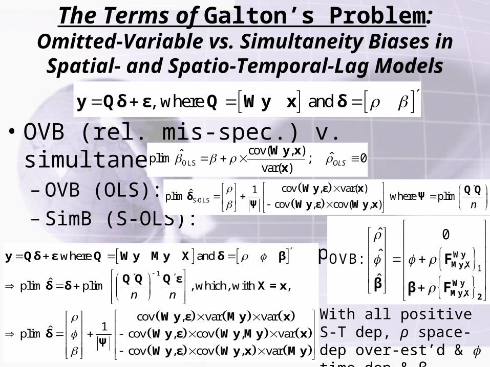
The Terms of Galton’s Problem:Omitted-Variable vs. Simultaneity Biases inSpatial- and Spatio-Temporal-Lag Models

• OVB (rel. mis-spec.) v. simultaneity:– OVB (OLS):

– SimB (S-OLS):

– In S-T, little more complicated, but:

, where and y Qδ ε Q Wy x δ

OLS

cov( , )ˆ ˆplim ; 0var( ) OLS

Wy x

x

S-OLS

cov , var( )1ˆplim where plimcov , cov( , ) n

Wy ε x Q Qδ Ψ

Wy ε Wy xΨ

1

where and

ˆplim plim , which, with ,

cov , var var1ˆplim cov , cov , var

cov , cov , var

n n

y Qδ ε Q Wy My X δ β

Q Q Q εδ δ X = x

Wy ε My x

δ Wy ε Wy My xΨ

Wy ε Wy x My

1

ˆ 0

ˆOVB:

ˆ

WyMy,X

WyMy,X 2

F

β β F

With all positive S-T dep, ρ space-dep over-est’d & time-dep & β under-est’d

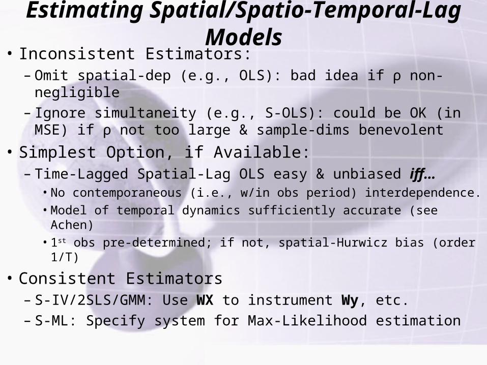
Estimating Spatial/Spatio-Temporal-Lag Models

• Inconsistent Estimators:– Omit spatial-dep (e.g., OLS): bad idea if ρ non-negligible– Ignore simultaneity (e.g., S-OLS): could be OK (in MSE)

if ρ not too large & sample-dims benevolent

• Simplest Option, if Available:– Time-Lagged Spatial-Lag OLS easy & unbiased iff…

• No contemporaneous (i.e., w/in obs period) interdependence.

• Model of temporal dynamics sufficiently accurate (see Achen)

• 1st obs pre-determined; if not, spatial-Hurwicz bias (order 1/T)

• Consistent Estimators– S-IV/2SLS/GMM: Use WX to instrument Wy, etc.– S-ML: Specify system for Max-Likelihood estimation

Estimating Spatial- & Spatio-Temporal-Dynamic Models by S-ML

• S-ML for Spatial-Lag Model:

– Std, but ε → y by |A| not 1 computational issues, plus

• Conditional S-ML S-T (ie., given 1stobs, Nx1 form); (unconditional is messy but exists; won’t show):

• Stationarity (if row-stdzd, & ρ,>0): ρ+<1• Spatial Probit: complicated but doable (show if time)• m-STAR & Est’d W; endog W: doable (show if…)

2

2 2

1( ) exp

2 2

NT

L

ε εy Wy XB ε ε I W y Xβ Ay Xβ ε

2

2 2

1 1( ) | | exp

2 2

NT

L

y A Ay Xβ Ay Xβ

1 2 1

2, ,..., 2

2

1

1 1ln 1 ln 2 1 ln

2 2

where ; was just:

t t

T

t tt

t t N t t N t t t N t t

f N T T

y y y y I W ε ε

ε y W y X β I y ε y W y X β

Figure 1: Estimated Bias in Plotted Against True Across Representative NxT Sample-Dimensions

Notes: Dashed Line: S-OLS. Dotted Line: S-2SLS-IV. Dashed-Dotted Line: S-ML

Figure 2: Estimated S Plotted Against True

Across Representative NxT Sample-Dimensions

Notes: Solid Line: Non-spatial OLS. Dashed Line: S-OLS. Dotted Line: S-2SLS-IV. Dashed-

Dotted Line: S-ML. Non-Spatial OLS results plotted against the larger-scale 2nd y-axis on the right.

Figure 3: RMSE Plotted Against True Across Representative NxT Sample-Dimensions (BIAS+EFFICIENCY)

Notes: Dashed Line: S-OLS. Dotted Line: S-2SLS-IV. Dashed-Dotted Line: S-ML.

Figure 4: RMSE S Plotted Against True Across Representative

NxT Sample-Dimensions (BIAS+EFFICIENCY)

Notes: Solid line: Non-spatial OLS. Dashed Line: S-OLS. Dotted Line: S-2SLS-IV. Dashed-Dotted

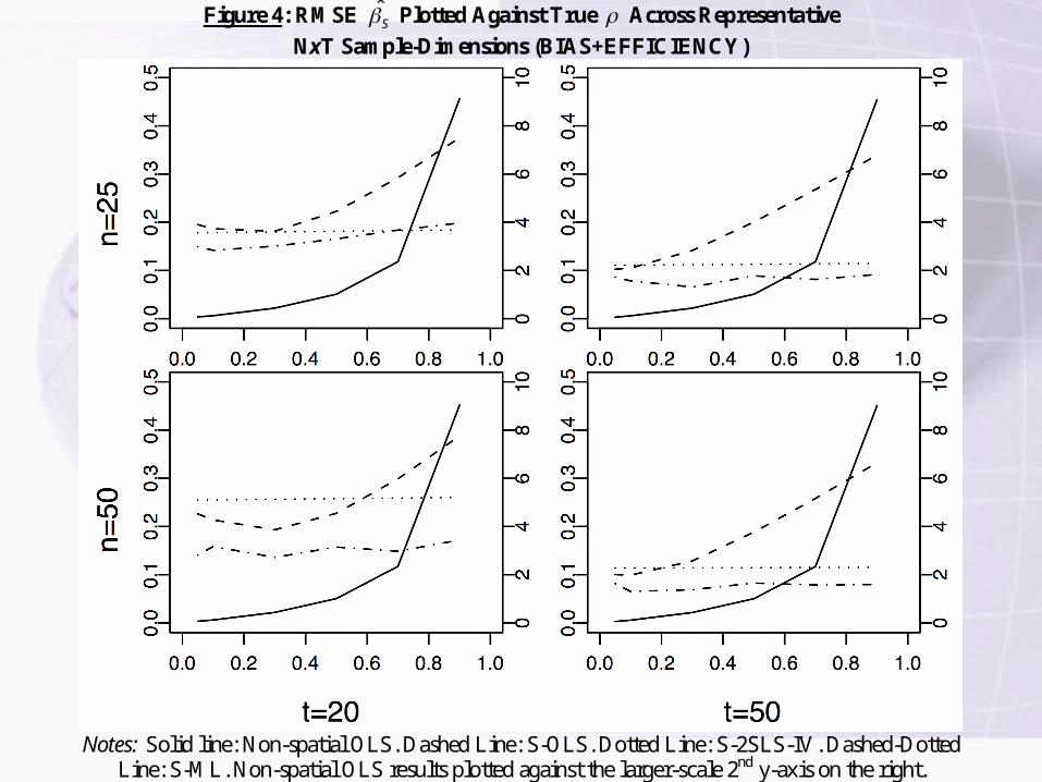
Line: S-ML. Non-spatial OLS results plotted against the larger-scale 2nd y-axis on the right.

Figure 5: Standard-Error Accuracy Plotted Against True Across Representative NxT Sample-Dimensions

Notes: Dashed Line: S-OLS. Dotted line: S-2SLS-IV. Dashed-Dotted Line: S-ML. Standard error accuracy is gauged by the ratio of the average estimated standard error to the true standard deviation of the sampling distribution. Values less than one indicate overconfidence.

Figure 6: Standard-Error S Accuracy Plotted Against True

Across Representative NxT Sample-Dimensions

Notes: Solid Line: Non-spatial OLS. Dashed Line: S-OLS. Dotted line: S-2SLS-IV. Dashed-Dotted Line: S-ML. Standard error accuracy is gauged by the ratio of the average estimated standard error to the sampling-distribution standard deviation. Values less than one indicate overconfidence.

APPLICATIONS• Globalization, Tax Competition, & Domestic Policy

– Replicates: Swank&Steinmo 02, Hays 03, Basinger&Hallerberg 04• ALMP: Active-Labor-Market Policy in EU (F&H ‘06)

– DepVar: LMT spend per unemployed worker– Hypoth: Positive spillovers (@ borders) effective member-state ALMP free-

riding & underinvest. Appreciable?– IndVars: rGDPpc, UE, UDen, Deindustrialization (Iversen-Soskice), Trade,

FDI, Pop65, LCab, CDemCab, LLibVote, GCons• MIDs & Trade: Beck, Gleditsch, & Beardsley ’06

– DepVar: Directed trade data;– Hypoth: MIDs affect trade in & beyond dyad– IndVars: GDPab, POPab, Distance, tau-b, MutualDem, MID, Bi/MultiPoleSys

• AFDC & CHIPs in U.S. States (Volden ’06)– AFDC: Hypoth—“states as laboratories”≈diffusion by learning

• DepVar: max monthly AFDC benefit• Ind Vars: state’s poverty rate, avg monthly wage in retail, govt ideology (0-100, R-

L), º interparty competition (.5-1.0, comp-non), tax effort (rev as % tax capacity), & % AFDC bens paid by fed govt.

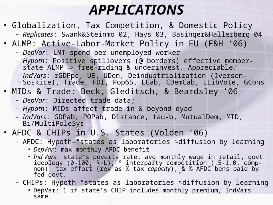
– CHIPs: Hypoth—“states as laboratories”≈diffusion by learning• DepVar: 1 if state’s CHIP includes monthly premium; IndVars same.

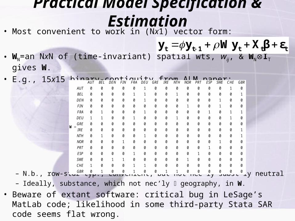
Practical Model Specification & Estimation• Most convenient to work in (Nx1) vector form:

• WN=an NxN of (time-invariant) spatial wts, wij, & WNIT gives W.

• E.g., 15x15 binary-contiguity from ALM paper:

– N.b., row-stdz typ., convenient, but not nec’ly subst’ly neutral

– Ideally, substance, which not nec’ly geography, in W.

• Beware of extant software: critical bug in LeSage’s MatLab code; likelihood in some third-party Stata SAR code seems flat wrong.

t t 1 t t ty y Wy X β ε

0 0 0 0 0 1 0 0 0 0 0 0 0 1 0

0 0 0 0 1 1 0 0 1 0 0 0 0 0 1

0 0 0 0 0 1 0 0 0 0 0 0 1 0 0

0 0 0 0 0 0 0 0 0 1 0 0 1 0 0

0 1 0 0 0 1 0 0 0 0 0 1 0 1 1

1 1 0 0 1 0 0 0 1 0 0 0 0 1 0

0 0 0 0 0 0 0 0 0 0 0 0 0 0 0

0 0 0 0 0 0 0 0 0 0 0 0 0 0 1

0 1 0 0 0 1

AUT BEL DEN FIN FRA DEU GRE IRE NTH NOR PRT ESP SWE CHE GBR

AUT

BEL

DEN

FIN

FRA

DEU

GRE

IRE

NTH

W

0 0 0 0 0 0 0 0 1

0 0 0 1 0 0 0 0 0 0 0 0 1 0 0

0 0 0 0 0 0 0 0 0 0 0 1 0 0 0

0 0 0 0 1 0 0 0 0 0 1 0 0 0 0

0 0 1 1 0 0 0 0 0 1 0 0 0 0 0

1 0 0 0 1 1 0 0 0 0 0 0 0 0 0

0 1 0 0 1 0 0 1 1 0 0 0 0 0 0

NOR

PRT

ESP

SWE

CHE

GBR

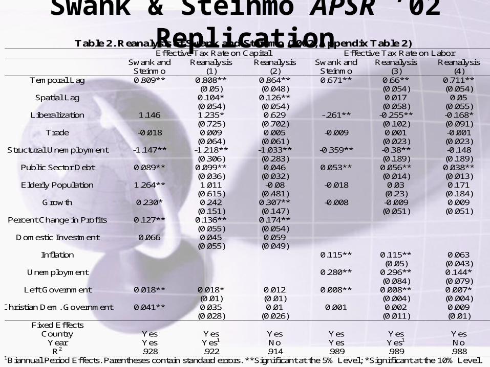
Swank & Steinmo APSR ’02 Replication

Table 2. Reanalysis of Swank and Steinmo (2002, Appendix Table 2) Effective Tax Rate on Capital Effective Tax Rate on Labor Swank and

Steinmo Reanalysis

(1) Reanalysis

(2) Swank and

Steinmo Reanalysis

(3) Reanalysis

(4) Temporal Lag 0.809** 0.808**

(0.05) 0.864** (0.048)

0.671** 0.66** (0.054)

0.711** (0.054)

Spatial Lag 0.104* (0.054)

0.126** (0.054)

0.017 (0.058)

0.05 (0.055)

Liberalization 1.146 1.235* (0.725)

0.629 (0.702)

-.261** -0.255** (0.102)

-0.168* (0.091)

Trade -0.018 0.009 (0.064)

0.005 (0.061)

-0.009 0.001 (0.023)

-0.001 (0.023)

Structural Unemployment -1.147** -1.218** (0.306)

-1.033** (0.283)

-0.359** -0.38** (0.189)

-0.148 (0.189)

Public Sector Debt 0.089** 0.099** (0.036)

0.046 (0.032)

0.053** 0.056** (0.014)

0.038** (0.013)

Elderly Population 1.264** 1.011 (0.615)

-0.08 (0.481)

-0.018 0.03 (0.23)

0.171 (0.184)

Growth 0.230* 0.242 (0.151)

0.307** (0.147)

-0.008 -0.009 (0.051)

0.009 (0.051)

Percent Change in Profits 0.127** 0.136** (0.055)

0.174** (0.054)

Domestic Investment 0.066 0.045 (0.055)

0.059 (0.049)

Inflation 0.115** 0.115** (0.05)

0.063 (0.043)

Unemployment 0.280** 0.296** (0.084)

0.144* (0.079)

Left Government 0.018** 0.018* (0.01)

0.012 (0.01)

0.008** 0.008** (0.004)

0.007* (0.004)

Christian Dem. Government 0.041** 0.035 (0.028)

0.01 (0.026)

0.001 0.002 (0.011)

0.009 (0.01)

Fixed Effects Country Yes Yes Yes Yes Yes Yes

Year Yes Yes1 No Yes Yes1 No R2 .928 .922 .914 .989 .989 .988

1Biannual Period Effects. Parentheses contain standard errors. **Significant at the 5% Level; *Significant at the 10% Level.

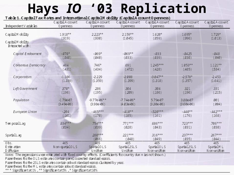
Hays IO ‘03 Replication

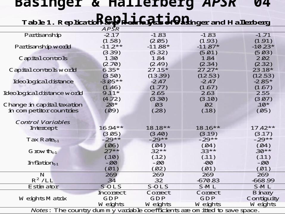
Basinger & Hallerberg APSR ’04 ReplicationTable 1. Replication and Reanalysis of Basinger and Hallerberg

APSR Partisanship -2.17

(1.58) -1.83 (2.05)

-1.83 (1.93)

-1.71 (1.91)

Partisanship world -11.2** (3.39)

-11.88* (5.32)

-11.87* (5.01)

-10.23* (5.03)

Capital controls 1.30 (2.70)

1.84 (2.49)

1.84 (2.34)

2.02 (2.32)

Capital controls world 6.35* (3.50)

27.15* (13.39)

27.27* (12.53)

23.18* (12.53)

Ideological distance -3.05** (1.46)

-2.47 (1.77)

-2.47 (1.67)

-2.85* (1.67)

Ideological distance world 9.11* (4.72)

2.65 (3.30)

2.63 (3.10)

2.55 (3.07)

Change in capital taxation in competitor countries

.20* (.09)

.03 (.28)

.02 (.18)

.10* (.05)

Control Variables

Intercept 16.94** (3.05)

18.18** (3.40)

18.16** (3.19)

17.42** (3.17)

Tax Ratet-1 -.29** (.06)

-.29** (.04)

-.29** (.04)

-.29** (.04)

Growtht-1 .27** (.10)

.32** (.12)

.33** (.11)

.30** (.11)

Inflationt-1 -.00 (.01)

-.00 (.02)

-00 (.01)

-.00 (.01)

N 269 269 269 269 R2 / LL .34 .32 -670.83 -668.99

Estimator S-OLS S-OLS S-ML S-ML

Weights Matrix Incorrect

GDP Weights

Correct GDP

Weights

Correct GDP

Weights

Binary Contiguity Weights

Notes: The country dummy variable coefficients are omitted to save space.

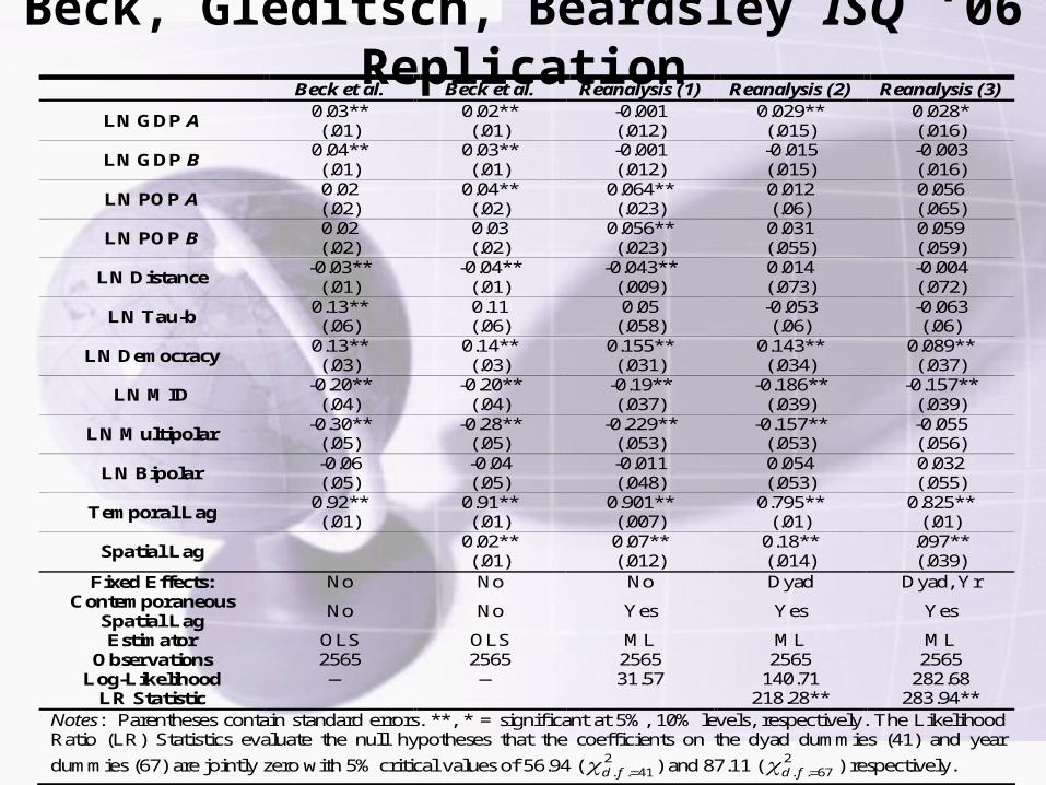
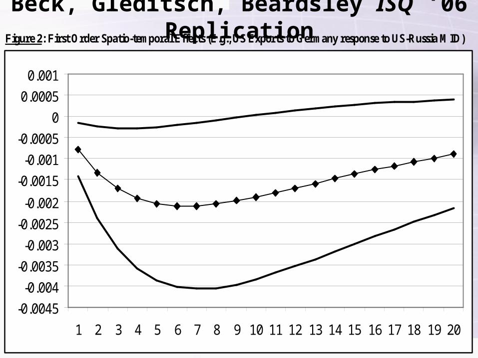
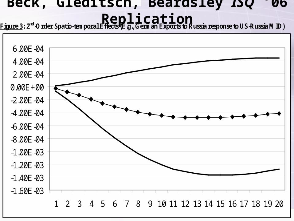
Beck, Gleditsch, Beardsley ISQ ‘06 Replication Beck et al. Beck et al. Reanalysis (1) Reanalysis (2) Reanalysis (3)

LN GDP A 0.03** (.01)

0.02** (.01)

-0.001 (.012)

0.029** (.015)

0.028* (.016)

LN GDP B 0.04** (.01)

0.03** (.01)

-0.001 (.012)

-0.015 (.015)

-0.003 (.016)

LN POP A 0.02 (.02)

0.04** (.02)

0.064** (.023)

0.012 (.06)

0.056 (.065)

LN POP B 0.02 (.02)

0.03 (.02)

0.056** (.023)

0.031 (.055)

0.059 (.059)

LN Distance -0.03**

(.01) -0.04**

(.01) -0.043**

(.009) 0.014 (.073)

-0.004 (.072)

LN Tau-b 0.13** (.06)

0.11 (.06)

0.05 (.058)

-0.053 (.06)

-0.063 (.06)

LN Democracy 0.13** (.03)

0.14** (.03)

0.155** (.031)

0.143** (.034)

0.089** (.037)

LN MID -0.20**

(.04) -0.20**

(.04) -0.19** (.037)

-0.186** (.039)

-0.157** (.039)

LN Multipolar -0.30**

(.05) -0.28**

(.05) -0.229**

(.053) -0.157**

(.053) -0.055 (.056)

LN Bipolar -0.06 (.05)

-0.04 (.05)

-0.011 (.048)

0.054 (.053)

0.032 (.055)

Temporal Lag 0.92** (.01)

0.91** (.01)

0.901** (.007)

0.795** (.01)

0.825** (.01)

Spatial Lag 0.02** (.01)

0.07** (.012)

0.18** (.014)

.097** (.039)

Fixed Effects: No No No Dyad Dyad, Yr Contemporaneous

Spatial Lag No No Yes Yes Yes

Estimator OLS OLS ML ML ML Observations 2565 2565 2565 2565 2565

Log-Likelihood — — 31.57 140.71 282.68 LR Statistic 218.28** 283.94**

Notes: Parentheses contain standard errors. **, * = significant at 5%, 10% levels, respectively. The Likelihood Ratio (LR) Statistics evaluate the null hypotheses that the coefficients on the dyad dummies (41) and year

dummies (67) are jointly zero with 5% critical values of 56.94 ( 2. . 41d f ) and 87.11 ( 2

. . 67d f ) respectively.

Franzese & Hays EUP ‘06

Volden AJPS ‘06 AFDC ReplicationTable 1. State Welfare Policy (Maximum AFDC Benefit)

Independent Variables

OLS

Spatial AR Lag (S-OLS)

Spatial AR Lag (S-2SLS)

Spatial AR Lag (S-GMM)

Spatial AR Lag (S-MLE)

Spatial AR Error (S-MLE)

Constant 54.519 (531.830)

-246.76 (450.75)

-422.09 (437.74)

-500.05 (413.02)

-156.282 (429.130)

676.120 (471.965)

Poverty Rate -6.560 (11.262)

8.04 (10.022)

13.205 (9.977)

7.29 (8.452)

3.657 (8.917)

3.239 (10.062)

Retail Wage -.121 (.226)

.016 (.193)

.089 (.187)

-.008 (.201)

-.025 (.181)

-.344 (.243)

Government Ideology 1.513 (1.030)

1.397 (.863)

1.359* (.825)

1.655** (.761)

1.432* (.806)

1.696** (.822)

Inter-party Competition 621.799** (290.871)

368.65 (250.55)

286.98 (243.72)

438.9** (197.47)

444.677* (226.911)

263.887 (238.419)

Tax Effort 3.357** (1.587)

2.022 (1.364)

1.553 (1.328)

2.397 (1.493)

2.423* (1.262)

2.936** (1.213)

Federal Share -4.405 (5.001)

-5.818 (4.20)

-6.012 (4.014)

-3.654 (3.415)

-5.393 (3.901)

-6.882* (4.099)

Spatial AR .767*** (.178)

1.069*** (.232)

.840*** (.237)

.537*** (.122)

.565*** (.131)

Moran I-statistic

3.312***

LM 12.322***

LM 11.606***

*LM 6.477**

LM 5.845***

*LM .716

Log-likelihood -270.763 -272.728 Adj.-R2 .461 .622 .595 .606 .510 .588

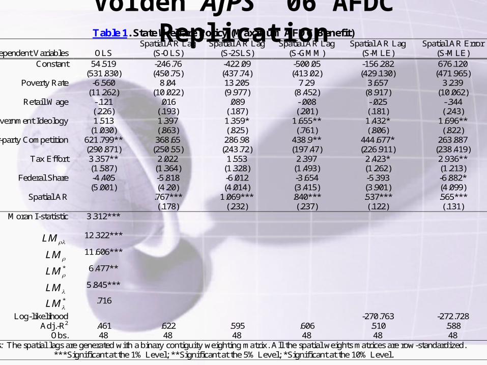
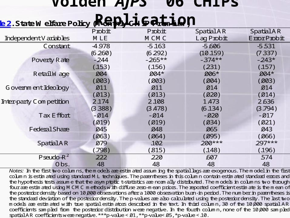
Obs. 48 48 48 48 48 48 Notes: The spatial lags are generated with a binary contiguity weighting matrix. All the spatial weights matrices are row-standardized.

***Significant at the 1% Level; **Significant at the 5% Level; *Significant at the 10% Level.

Volden AJPS ‘06 CHIPs ReplicationTable 2. State Welfare Policy (Monthly CHIP Premium)

Independent Variables

Probit MLE

Probit MCMC

Spatial AR Lag Probit

Spatial AR Error Probit

Constant -4.978 (6.260)

-5.163 (6.292)

-5.606 (10.159)

-5.531 (7.337)

Poverty Rate -.244 (.153)

-.265** (.156)

-.374** (.231)

-.243* (.157)

Retail Wage .004 (.003)

.004* (.003)

.006* (.004)

.004* (.003)

Government Ideology .011 (.013)

.011 (.013)

.014 (.020)

.014 (.014)

Inter-party Competition 2.174 (3.388)

2.108 (3.478)

1.473 (6.134)

2.636 (3.794)

Tax Effort -.014 (.019)

-.014 (.019)

-.020 (.034)

-.017 (.021)

Federal Share .045 (.063)

.048 (.064)

.065 (.095)

.043 (.066)

Spatial AR .079 (.798)

.102 (.815)

.200*** (.148)

.297*** (.196)

Pseudo-R2 .222 .220 .607 .574 Obs. 48 48 48 48

Notes: In the first two columns, the models are estimated assuming the spatial lags are exogenous. The model in the first column is estimated using standard ML techniques. The parentheses in this column contain estimated standard errors and the hypothesis tests assume that the asymptotic t-statistics are normally distributed. The models in columns two through four are estimated using MCMC methods with diffuse zero-mean priors. The reported coefficient estimate is the mean of the posterior density based on 10,000 observations after a 1000 observation burn-in period. The number in parentheses is the standard deviation of the posterior density. The p-values are also calculated using the posterior density. The last two models are estimated with true spatial estimators described in the text. In third column, 30 of the 10,000 spatial AR coefficients sampled from the posterior distribution were negative. In the fourth column, none of the 10,000 sampled spatial AR coefficients were negative. ***p-value <.01, **p-value<.05, *p-value <.10.

Interpreting Spatial/Spatio-Temporal Effects• The Model:

– Model may look linear, but is not; as in all beyond purely linear-additive, coefficients & effects very different things!

– Convenient, for interpretation, to write model this way too:

– Coefficients, βx are just pre-spatial, pre-temporal—and wholly unobservable!—impulse from some x to y.

• Spatio-Temporal Effects:– Post-spatial, pre-temporal “instantaneous effect” of x:

– Spatio-Temporal Response Paths:

– LR Multiplier/LR-SS:

y Wy My Xβ ε

1t N t t t t y W y y X β ε

1

1t N N t t t y I W y X β ε

1 1 for some (set of) ; i.e., c i

N N t t i N N kx i I W X β ε I W x β

1

N N

t t t t t t t t

t t

y Wy y X β ε W I y X β ε

I W I X β ε

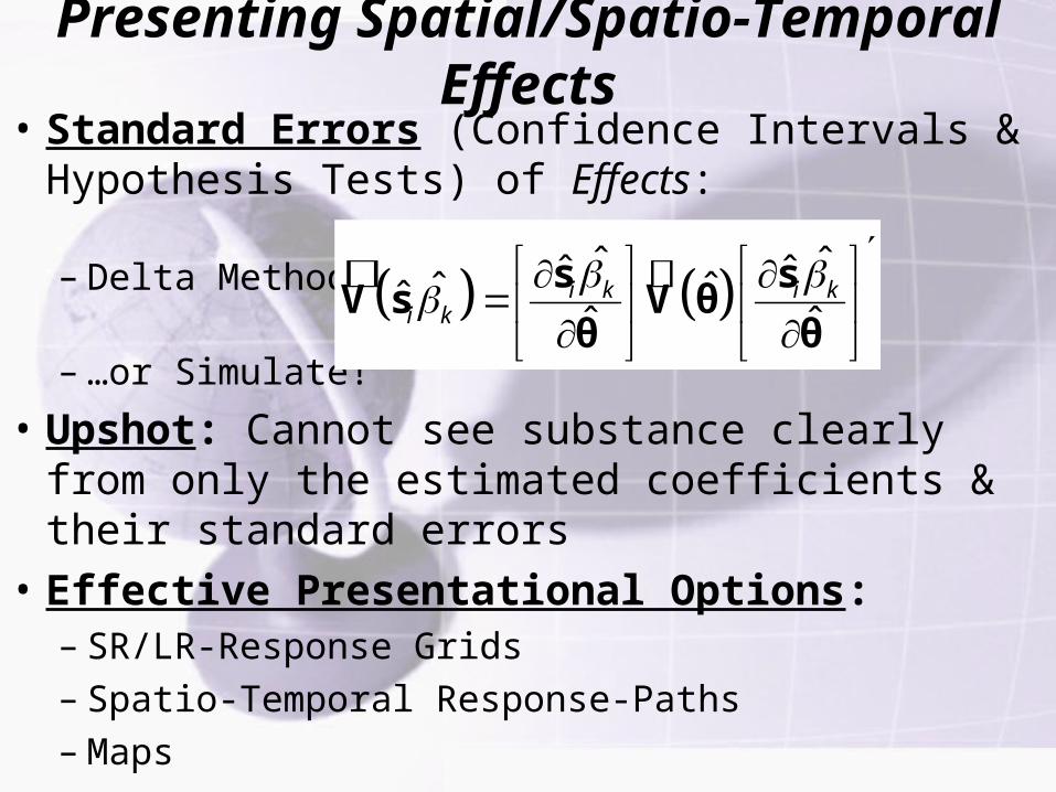
Presenting Spatial/Spatio-Temporal Effects• Standard Errors (Confidence Intervals &

Hypothesis Tests) of Effects:

– Delta Method:

– …or Simulate!

• Upshot: Cannot see substance clearly from only the estimated coefficients & their standard errors

• Effective Presentational Options:– SR/LR-Response Grids– Spatio-Temporal Response-Paths– Maps

ˆ ˆˆ ˆˆ ˆˆˆ ˆ

i k i ki k

s sV s V θ

θ θ

Swank & Steinmo APSR ’02 Replication

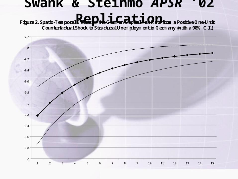
Swank & Steinmo APSR ’02 ReplicationFigure 2. Spatio-Temporal Effects on the German Capital Tax Rate from a Positive One-Unit

Counterfactual Shock to Structural Unemployment in Germany (with a 90% C.I.)

-2

-1.8

-1.6

-1.4

-1.2

-1

-0.8

-0.6

-0.4

-0.2

0

0.2

1 2 3 4 5 6 7 8 9 10 11 12 13 14 15

Cumulative 15-Period Effect: -6.523

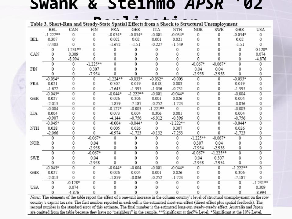
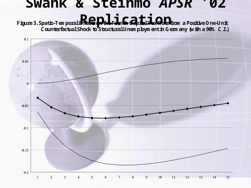
Swank & Steinmo APSR ’02 ReplicationFigure 3. Spatio-Temporal Effects on the French Capital Tax Rate from a Positive One-Unit

Counterfactual Shock to Structural Unemployment in Germany (with a 90% C.I.)

-0.2

-0.15

-0.1

-0.05

0

0.05

0.1

1 2 3 4 5 6 7 8 9 10 11 12 13 14 15

Cumulative 15-Period Effect: -.943

Basinger & Hallerberg APSR ’04 Replication

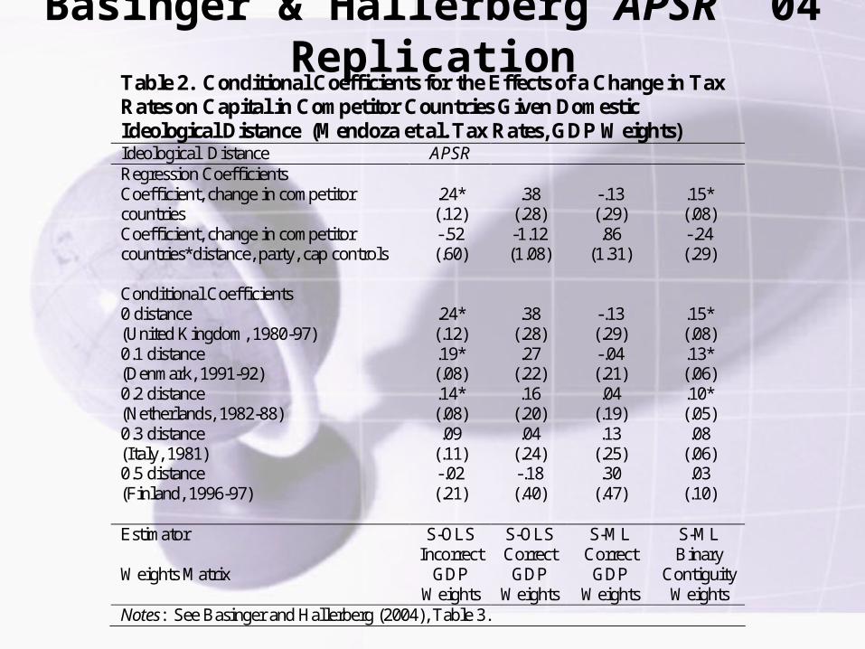
Table 2. Conditional Coefficients for the Effects of a Change in Tax Rates on Capital in Competitor Countries Given Domestic Ideological Distance (Mendoza et al. Tax Rates, GDP Weights) Ideological Distance APSR Regression Coefficients Coefficient, change in competitor countries

.24* (.12)

.38 (.28)

-.13 (.29)

.15* (.08)

Coefficient, change in competitor countries*distance, party, cap controls

-.52 (.60)

-1.12 (1.08)

.86 (1.31)

-.24 (.29)

Conditional Coefficients 0 distance (United Kingdom, 1980-97)

.24* (.12)

.38 (.28)

-.13 (.29)

.15* (.08)

0.1 distance (Denmark, 1991-92)

.19* (.08)

.27 (.22)

-.04 (.21)

.13* (.06)

0.2 distance (Netherlands, 1982-88)

.14* (.08)

.16 (.20)

.04 (.19)

.10* (.05)

0.3 distance (Italy, 1981)

.09 (.11)

.04 (.24)

.13 (.25)

.08 (.06)

0.5 distance (Finland, 1996-97)

-.02 (.21)

-.18 (.40)

.30 (.47)

.03 (.10)

Estimator S-OLS S-OLS S-ML S-ML Weights Matrix

Incorrect GDP

Weights

Correct GDP

Weights

Correct GDP

Weights

Binary Contiguity Weights

Notes: See Basinger and Hallerberg (2004), Table 3.

Basinger & Hallerberg APSR ’04 Replication Table 3. Conditional Coefficients for the Effects of a Change in Tax Rates on Capital in Competitor Countries Given Domestic Partisanship Level (Mendoza et al. Tax Rates, GDP Weights) Partisanship APSR Regression Coefficients Coefficient, change in competitor countries

-.24 (.40)

1.39* (.71)

-.83 (.89)

-.11 (.21)

Coefficient, change in competitor countries*distance, party, cap controls

.67 (.63)

-2.13* (1.21)

1.47 (1.52)

.40 (.37)

0 partisanship (no country)

-.24 (.40)

1.39* (.71)

-.83 (.89)

-.11 (.21)

0.2 partisanship (Norway, 1989)

-.10 (.27)

.96* (.48)

-.54 (.60)

-.03 (.14)

0.4 partisanship (Netherlands, 1982-88)

.03 (.16)

.53* (.28)

-.24 (.32)

.05 (.07)

0.6 partisanship (Austria, 1987-97)

.16* (.07)

.10 (.21)

.05 (.19)

.13* (.06)

0.8 partisanship (Ireland, 1990-92)

.30* (.13)

-.32 (.36)

.35 (.39)

.21* (.11)

Estimator S-OLS S-OLS S-ML S-ML Weights Matrix

Incorrect GDP

Weights

Correct GDP

Weights

Correct GDP

Weights

Binary Contiguity Weights

Notes: See Basinger and Hallerberg (2004), Table 4.

Table 4. Conditional Coefficients for the Effects of a Change in Tax Rates on Capital in Competitor Countries Given Domestic Use of Capital Controls (Mendoza et al. Tax Rates, GDP Weights) Capital Controls APSR Regression Coefficients Coefficient, change in competitor countries

.26* (.10)

.11 (.28)

.16 (.21)

.08 (.06)

Coefficient, change in competitor countries*distance, party, cap controls

-.96 (.76)

.60 (1.86)

-1.88 (1.51)

.20 (.33)

0 capital controls (United States, 1980-97)

.26* (.10)

.11 (.28)

.16 (.21)

.08 (.06)

0.25 capital controls (France, 1980-89)

.02 (.14)

.26 (.35)

-.31 (.33)

.13* (.07)

0.5 capital controls (Portugal, 1980-85)

-.22 (.32)

.41 (.77)

-.78 (.68)

.18 (.14)

0.75 capital controls (Greece, 1981)

-.46 (.50)

.56 (1.23)

-1.25 (1.05)

.23 (.22)

Estimator S-OLS S-OLS S-ML S-ML Weights Matrix

Incorrect GDP

Weights

Correct GDP

Weights

Correct GDP

Weights

Binary Contiguity Weights

Notes: See Basinger and Hallerberg (2004), Table 5.

Beck, Gleditsch, Beardsley ISQ ‘06 Replication Figure 1: Temporal Effects with Spatial Feedback (E.g., US Exports to Russia response to US-Russia MID)

-0.25

-0.2

-0.15

-0.1

-0.05

0

1 2 3 4 5 6 7 8 9 10 11 12 13 14 15 16 17 18 19 20

Beck, Gleditsch, Beardsley ISQ ‘06 Replication Figure 2: First Order Spatio-temporal Effects (E.g., US Exports to Germany response to US-Russia MID)

-0.0045

-0.004

-0.0035

-0.003

-0.0025

-0.002

-0.0015

-0.001

-0.0005

0

0.0005

0.001

1 2 3 4 5 6 7 8 9 10 11 12 13 14 15 16 17 18 19 20

Beck, Gleditsch, Beardsley ISQ ‘06 ReplicationFigure 3: 2nd-Order Spatio-temporal Effects (E.g., German Exports to Russia response to US-Russia MID)

-1.60E-03

-1.40E-03

-1.20E-03

-1.00E-03

-8.00E-04

-6.00E-04

-4.00E-04

-2.00E-04

0.00E+00

2.00E-04

4.00E-04

6.00E-04

1 2 3 4 5 6 7 8 9 10 11 12 13 14 15 16 17 18 19 20

Franzese & Hays EUP ‘06

Franzese & Hays EUP ‘06Table 3. Steady-State Spatial Effects of labor Market Training Expenditures in Europe (Binary Contiguity Weights Matrix) AUT BEL DEN FIN FRA DEU IRE NTH NOR PRT ESP SWE CHE GBR 0.027 0.052 0.002 0.159 -0.530* 0.005 0.050 0.002 0.006 -0.021 -0.016 -0.557* -0.033 AUT (.0136) (.0296) (.0024) (.0914) (.1588) (.0050) (.0292) (.0024) (.0067) (.0189) (.0134) (.1663) (.0277) 0.013 0.023 0.001 -0.254* -0.238* 0.033 -0.236* 0.001 -0.009 0.033 -0.007 0.047 -0.237* BEL (.0068) (.0125) (.0010) (.0723) (.0636) (.0167) (.0581) (.0010) (.0079) (.0204) (.0058) (.0237) (.0636) 0.052 0.047 0.094 0.051 -0.640* 0.003 0.056 0.094 0.002 -0.007 -0.648* 0.039* -0.025 DEN (.0407) (.0346) (.0505) (.0305) (.2218) (.0038) (.0335) (.0505) (.0022) (.0062) (.2271) (.0183) (.0211) 0.002 0.002 0.094 0.002 -0.028 0.000 0.002 -0.520* 0.000 0.000 -0.493* 0.002 -0.001 FIN (.0785) (.0640) (.0739) (.0570) (.2043) (.0096) (.0621) (.0076) (.0057) (.0149) (.0403) (.0266) (.0489) 0.064* -0.203* 0.020 0.001 -0.207* 0.034 0.082* 0.001 0.080* -0.286* -0.006 -0.240* -0.247* FRA (.0031) (.0027) (.0505) (.2121) (.0228) (.0002) (.0026) (.1477) (.0001) (.0004) (.1402) (.0016) (.0014) -0.177* -0.158 -0.213* -0.009 -0.173 -0.012 -0.191* -0.009 -0.006 0.023 0.065 -0.133 0.083 DEU (.0502) (.0864) (.0122) (.0010) (.2112) (.0209) (.0466) (.0010) (.0514) (.1164) (.0054) (.0808) (.0910) 0.009 0.132 0.007 0.000 0.172 -0.069 0.163 0.000 0.006 -0.023 -0.002 -0.015 -1.257* IRE (.0131) (.0928) (.0075) (.0005) (.1045) (.0576) (.0940) (.0005) (.0074) (.0212) (.0029) (.0127) (.4242) 0.033 -0.314* 0.038 0.002 0.137 -0.382* 0.054 0.002 0.005 -0.018 -0.011 0.011 -0.390* NTH (.0267) (.1186) (.0223) (.0018) (.0777) (.1241) (.0313) (.0018) (.0057) (.0161) (.0099) (.0007) (.1319) 0.002 0.002 0.094 -0.520* 0.002 -0.028 0.000 0.002 0.000 0.000 -0.493* 0.002 -0.001 NOR (.0031) (.0027) (.0505) (.1477) (.0024) (.0228) (.0002) (.0026) (.0001) (.0004) (.1402) (.0016) (.0014) 0.012 -0.037 0.004 0.000 0.398 -0.038 0.006 0.015 0.000 -1.345* -0.001 -0.044 -0.045 PRT (.0175) (.0424) (.0044) (.0003) (.2572) (.0341) (.0074) (.0171) (.0003) (.5073) (.0016) (.0398) (.0425) -0.021 0.067 -0.007 0.000 -0.714* 0.068 -0.011 -0.027 0.000 -0.672* 0.002 0.079 0.082 ESP (.0252) (.0559) (.0062) (.0004) (.2910) (.0448) (.0106) (.0242) (.0004) (.2537) (.0025) (.0524) (.0566) -0.011 -0.009 -0.432* -0.329* -0.010 0.129 -0.001 -0.011 -0.329* 0.000 0.001 -0.008 0.005 SWE (.0119) (.0103) (.1514) (.0935) (.0090) (.0805) (.0010) (.0099) (.0935) (.0005) (.0016) (.0059) (.0056) -0.371* 0.062 0.026 0.001 -0.400* -0.266* -0.005 0.011 0.001 -0.015 0.053 -0.008 0.037 CHE (.1644) (.0439) (.0122) (.0011) (.1346) (.0532) (.0042) (.0007) (.0011) (.0133) (.0350) (.0059) (.0217) -0.017 -0.237* -0.012 -0.001 -0.309* 0.125 -0.314* -0.293* -0.001 -0.011 0.041 0.004 0.028 GBR (.0185) (.0959) (.0105) (.0007) (.1137) (.0734) (.1061) (.0989) (.0007) (.0106) (.0283) (.0042) (.0163) Notes: The off-diagonal elements of the table report the effect of a one-unit increase in the column country’s labor-market-training expenditures on its European

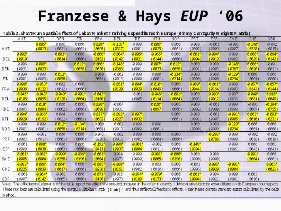
counterparts. These numbers are calculated using the long-run spatio-temporal-multiplier matrix 111 WIW)(II . Parentheses contain standard errors

calculated by the delta method.

Some Other Presentations (3)

+1 Shock to Germany

-0.748 - -0.649

-0.648 - -0.549

-0.548 - -0.449

-0.448 - -0.349

-0.348 - -0.249

-0.248 - -0.220

-0.219 - -0.149

-0.148 - -0.049

-0.048 - 0.015

0.016 - 0.049

0.050 - 0.149

+1 Shock to Germany

-0.748 - -0.649

-0.648 - -0.549

-0.548 - -0.449

-0.448 - -0.349

-0.348 - -0.249

-0.248 - -0.220

-0.219 - -0.149

-0.148 - -0.049

-0.048 - 0.015

0.016 - 0.049

0.050 - 0.149

Figure 1. Short-run Spatial Effects of a Positive One-unit Shock to German LMT Expenditures

Figure 2. Steady-state Spatial Effects of a Positive One-unit Shock to German LMT Expenditures

Volden AJPS ‘06 AFDC Replication Table 4. Spatial Effects on AFDC Benefits from a $100 Counterfactual Shock to Monthly Retail Wages in Missouri Neighbor

Immediate Spatial Effect

Long-Run Steady State Effect

Arkansas

.51 [.16,.87]

4.26 [1.01,7.52]

Illinois

.62 [.19,1.04]

5.11 [1.25,8.97]

Iowa

0.52 [.15,.88]

4.37 [.99, 7.75]

Kansas

0.77 [.23,1.31]

6.38 [1.60,11.17]

Kentucky

0.44 [.13,.75]

3.68 [.87,6.50]

Nebraska

0.52 [.15,.89]

4.44 [.99,7.90]

Oklahoma

0.52 [.15,.89]

4.47 [.96,7.98]

Tennessee

0.38 [.12,.65]

3.21 [.75,5.67]

Notes: Effects calculated using estimates from the spatial AR lag model in Table 3. Brackets contain a 95% confidence interval.

Volden AJPS ‘06 AFDC ReplicationFigure 1. Spatio-Temporal Effects on AFDC Benefits in Missouri from a

$100 Counterfactual Shock to Monthly Retail Wages in Missouri (with 95% C.I.)

0

5

10

15

20

25

30

1 2 3 4 5 6 7 8 9 10

Cumulative 10-Period Effect: $55.75

Volden AJPS ‘06 AFDC ReplicationFigure 2. Spatio-Temporal Effects on AFDC Benefits in Nebraska from a

$100 Counterfactual Shock to Monthly Retail Wages in Missouri (with 95% C.I.)

0

0.2

0.4

0.6

0.8

1

1.2

1.4

1 2 3 4 5 6 7 8 9 10

Cumulative 10-Period Effect: $4.11

Conclusion• Spatial & Spatio-Temporal Interdependence

– Important & Appreciable Substance (e.g., globalization & int’l cap-tax compete seems quite real & does constrain), not Nuisance.

• Therefore: Model them. Interpret them.

• How specify & estimate models?– If space-lag is time-lagged, not problem; but if thry & substance

says immediate (w/in an observational period), can handle that too:– S-OLS not a bad strategy even then, if ρ not too big & smpl-dims

right; S-ML, & in some regards IV-based strategies, seem effective

• Spatio-Temporal Effects not directly read from coefficients: use graphs & maps & grids

• Information-demands of Galton’s Problem severe – Standard errors of effects tend big. Suspect delta-method lin-

approx. maybe part problem; plan explore performance bootstrap.– Max effort & care theory, measure, specification, to both C&IPE

Spatial QualDep: The Econometric Problem (1)• Spatial Qualitative/Categorical/Lmtd-Dep-Var Models in the Lit:

– Spatial probit: McMillen 1992,1995; Bolduc et. al. 1997; Pinkse & Slade 1998; LeSage 1999, 2000; Beron et al. 2003; Beron & Vijverberg 2004

• Spatial logit: Dubin 1997; Lin 2003; Autant-Bernard 2006• Spatial sample-selection (i.e., s-Tobit/Heckit): McMillen 1995, Smith & LeSage

2004, Flores-Lagunes & Schnier 2006• Spatial multinomial-probit: McMillen 1995, Bolduc et al. 1997• Spatial discrete-duration: Phaneuf & Palmquist 2003• Survival w/ spatial frailty: Banerjee et al. 2004, Darmofal 2007• Spatial count: Bhati 2005, including ZIP: Rathbun & Fei 2006

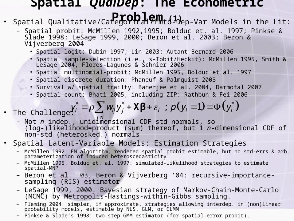
• The Challenge:– Not n indep., unidimensional CDF std normals, so

(log-)likelihood=product (sum) thereof, but 1 n-dimensional CDF of non-std (heterosked.) normals

• Spatial Latent-Variable Models: Estimation Strategies– McMillen 1992: EM algorithm, rendered spatial probit estimable, but no std-errs & arb.

parameterization of induced heteroscedasticity.– McMillen 1995, Bolduc et. al. 1997: simulated-likelihood strategies to estimate spatial-MNP– Beron et al. ‘03, Beron & Vijverberg ‘04: recursive-importance-sampling

(RIS) estimator– LeSage 1999, 2000: Bayesian strategy of Markov-Chain-Monte-Carlo

(MCMC) by Metropolis-Hastings-within-Gibbs sampling.– Fleming 2004: simpler, if approximate, strategies allowing interdep. in (non)linear probability

models, estimable by NLS, GLM, or GLMM– Pinkse & Slade’s 1998: two-step GMM estimator (for spatial-error probit).

* * * ; 1i ij j i i ij i

y w y p y y

Xβ

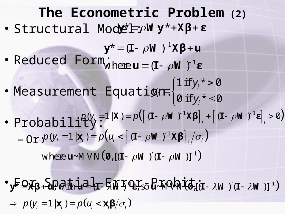
• Structural Model:

• Reduced Form:

• Measurement Equation:

• Probability:– Or:

• For Spatial-Error-Probit:

The Econometric Problem (2)* * y Wy Xβ ε

1

1

* ( )

where ( )

y I W Xβ u

u I W ε

1 if * 0

0 if * 0i

ii

yy

y

1 1( 1| ) ( ) ( ) 0i i ip y p X I W Xβ I W ε

1

1

( 1| ) ( )

where ~MVN ,[( ) ( )]

i i i iip y p u

x I W Xβ

u 0 I W I W

1 1* ; with ( ) , so ~MVN ,[( ) ( )]

( 1| )i i i i ip y p u

y Xβ u u I W ε u 0 I W I W

x x β

• Comments:– Notice that, when we come to interpret & , we face

the same MVN integration• We haven’t seen such substantive interpretation yet attempted

fully in the literature, but we suggest an easier way to do it.

– If can order dependence pattern & ensure only antecedent y* appear on RHS, then std probit ML w/ a spatial-lag works

• We think usu. indefensible subst’ly/thry’ly, but cf. Swank on capital-tax competition, e.g., where argues US exclusively leads & omits US.

– Having y, not y*, on RHS may seem subst’ly or thry’ly desirable in some cases, but gen’ly not logically possible:

• Problem would be that outcome, yi, would indirectly (via spatial feedback) determine yi

*, but then yi* would directly determine yi.

The stochastic difference b/w them will thus a logical inconsistency.

– Notice similar MVN issue w/ time lags; suggests similar strategies (but simpler b/c ordered) may allow model temp dynamics directly rather than nuisance (e.g., BKT splines)

The Econometric Problem (3)

p pD

DX

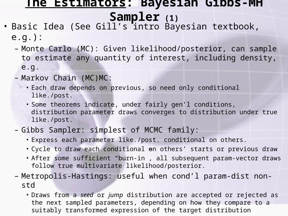
• Basic Idea (See Gill’s intro Bayesian textbook, e.g.):– Monte Carlo (MC): Given likelihood/posterior, can sample to

estimate any quantity of interest, including density, e.g.– Markov Chain (MC)MC:

• Each draw depends on previous, so need only conditional like./post.• Some theorems indicate, under fairly gen’l conditions, distribution

parameter draws converges to distribution under true like./post.

– Gibbs Sampler: simplest of MCMC family:• Express each parameter like./post. conditional on others.• Cycle to draw each conditional on others’ starts or previous draw• After some sufficient “burn-in”, all subsequent param-vector draws

follow true multivariate likelihood/posterior.

– Metropolis-Hastings: useful when cond’l param-dist non-std• Draws from a seed or jump distribution are accepted or rejected as

the next sampled parameters, depending on how they compare to a suitably transformed expression of the target distribution

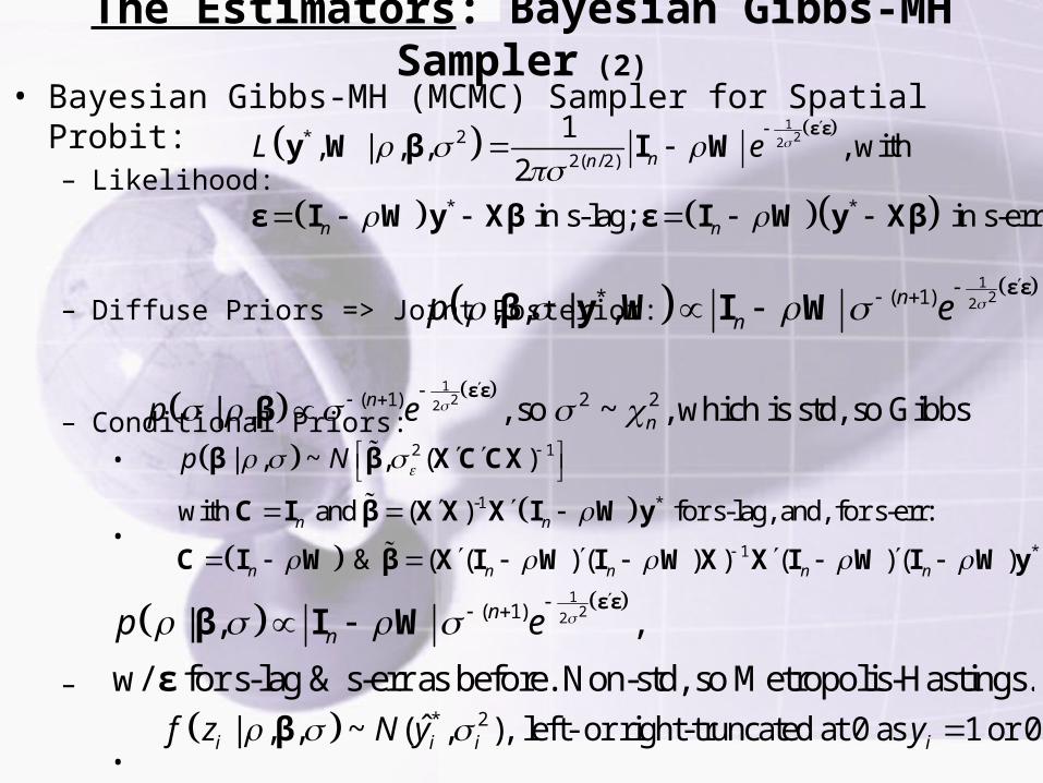
The Estimators: Bayesian Gibbs-MH Sampler (1)

• Bayesian Gibbs-MH (MCMC) Sampler for Spatial Probit:– Likelihood:

– Diffuse Priors => Joint Posterior:

– Conditional Priors:•

•

–

•

The Estimators: Bayesian Gibbs-MH Sampler (2)

122* 2

2( /2)

* *

1, | , , , with

2

in s-lag; in s-err

nn

n n

L e

ε εy W β I W

ε I W y Xβ ε I W y Xβ

122* ( 1), , | , n

np e

ε εβ y W I W

122( 1) 2 2| , , so ~ , which is std, so Gibbsn

np e

ε εβ

2 1

-1 *

1 *

| , ~ , ( )

with and ( ) for s-lag, and, for s-err:

& ( ( ) ( ) ) ( ) ( )

n n

n n n n n

p N

β β X C CX

C I β X X X I W y

C I W β X I W I W X X I W I W y

122( 1)| , ,

w/ for s-lag & s-err as before. Non-std, so Metropolis-Hastings.

nnp e

ε ε

β I W

ε

* 2ˆ| , , ~ ( , ), left- or right-truncated at 0 as 1 or 0i i i if z N y y β

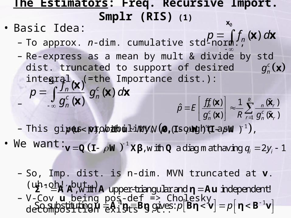
• Basic Idea:– To approx. n-dim. cumulative std-norm.,– Re-express as a mean by mult & divide by std dist.

truncated to support of desired integral, (=the Importance dist.):

–

– This gives probability, p, sought as:

• We want:

– So, Imp. dist. is n-dim. MVN truncated at v. (uh-oh! but…)

– V-Cov u being pos-def => Cholesky decomposition exists s.t.:

The Estimators: Freq. Recursive Import. Smplr (RIS) (1)

0

( ) np f d

x

x x

cng x

0 ( ) ( )

( )cnnc

n

fp g d

g

x

xx x

x1

( ) ( )1ˆ

( ) ( )

Rn n rc c

rn n r

f fp E

g R g

x x

x x

1

1

( ), with ~ , ( ) ( ) ,

, with a diag mat having 2 1i i

p MVN

q y

u v u 0 I W I W

v Q I W Xβ Q

1

1

, with upper-triangular and independent!

So substituting gives: p p

-1

Σ A A A η Au

u A η Bη Bη v η B v

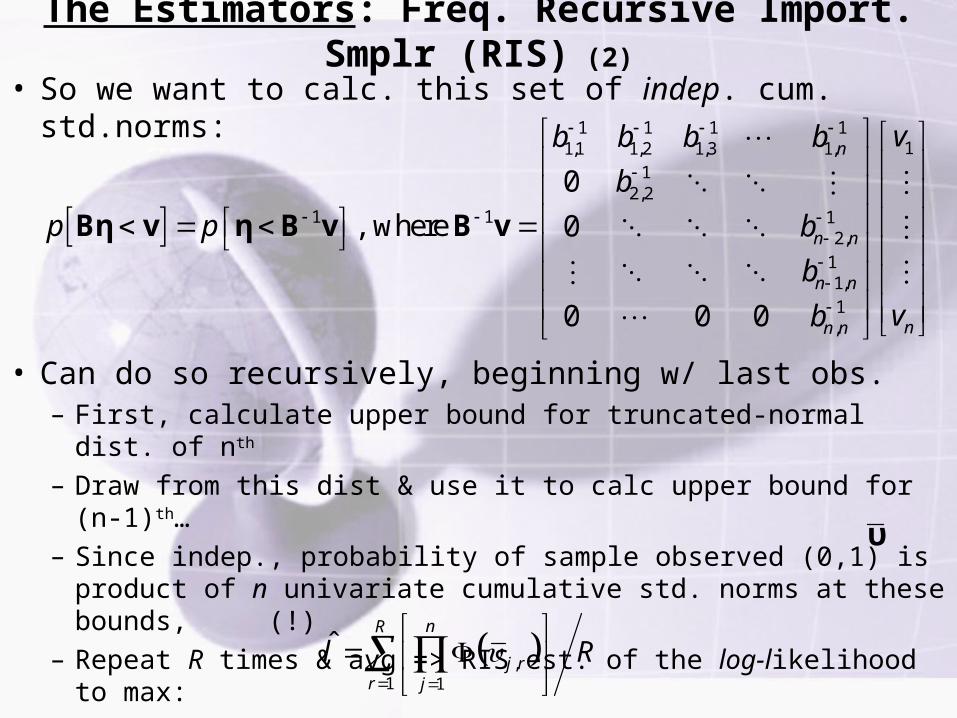
• So we want to calc. this set of indep. cum. std.norms:

• Can do so recursively, beginning w/ last obs.– First, calculate upper bound for truncated-normal dist. of

nth

– Draw from this dist & use it to calc upper bound for (n-1)th…

– Since indep., probability of sample observed (0,1) is product of n univariate cumulative std. norms at these bounds, (!)

– Repeat R times & avg => RIS est. of the log-likelihood to max:

The Estimators: Freq. Recursive Import. Smplr (RIS) (2)

1 1 1 111,1 1,2 1,3 1,

12,2

1 1 12,

11,1,

0

, where 0

0 0 0

n

n n

n n

nn n

vb b b b

b

p p b

b

vb

Bη v η B v B v

,1 1

ˆnR

j rr j

l R

υ

Evaluating the Estimators (One Quick MC)

• DGF: (n.b., same W, diff. coeffs. For x & y)

• Conditions:– Row-stdzd contig. wts U.S. 48; =0.5, =1.0,

n={48,144},θ={0.0, 0.5}

• You can’t see this, but:– Rel’ly poor bias perf. BG– In fact, std ML w/ Wy– seems dominate, but this– b/c 2 biases, meas./spec.– err & simult. Simult incr– in , meas-err decr or flat– in n, so over- to under-est.– (Checked & it’s true) B&V ‘04– do MC like #2 for RIS & find =-18%, =+10%, so better.

1 1* , where and , ~ 0,1n n N y I W x β ε x I W z z ε

ML with Wy ML with Wy* Bayesian Gibbs

Experiment #1: n=48, =0.0 Mean Coefficient Estimate 1.02 0.32 1.13 0.74 1.23 0.30 Actual SD of Estimates 0.33 0.69 0.41 0.36 0.28 0.16 Mean of Reported SE 0.30 0.41 0.35 0.30 0.42 0.21 Experiment #2: n=48, =0.5 Mean Coefficient Estimate 1.22 0.35 1.13 0.69 1.21 0.28 Actual SD of Estimates 0.56 0.76 0.61 0.33 0.24 0.14 Mean of Reported SE 0.36 0.46 0.42 0.29 0.39 0.20 Experiment #3: n=144, =0.0 Mean Coefficient Estimate 0.94 0.42 1.01 0.68 1.14 0.34 Actual SD of Estimates 0.17 0.27 0.19 0.16 0.15 0.10 Mean of Reported SE 0.16 0.22 0.18 0.15 0.22 0.12 Experiment #4: n=144, =0.5 Mean Coefficient Estimate 1.08 0.48 0.97 0.64 1.13 0.32 Actual SD of Estimates 0.19 0.29 0.21 0.16 0.14 0.09 Mean of Reported SE 0.18 0.23 0.20 0.15 0.21 0.12

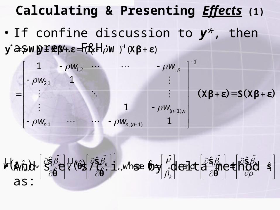
Calculating & Presenting Effects (1)

• If confine discussion to y*, then as prev. F&H:

• And s.e.’s/c.i.’s by delta method as:

* -1

1

1,2 1,

2,1

( 1),

,1 ,( 1)

( ) ( )

1

1

1

1

n

n

n n

n n n

w w

w

w

w w

y Wy Xβ ε I W Xβ ε

Xβ ε S Xβ ε

ˆ ˆ ˆ ˆ ˆˆ ˆ ˆ ˆˆ ˆ ˆˆ ˆ, where and ˆ ˆ ˆ ˆ ˆ

i k i k i k i ki k i

k

V V

s s s ss θ θ s

θ θ θ

Calculating & Presenting Effects (2)

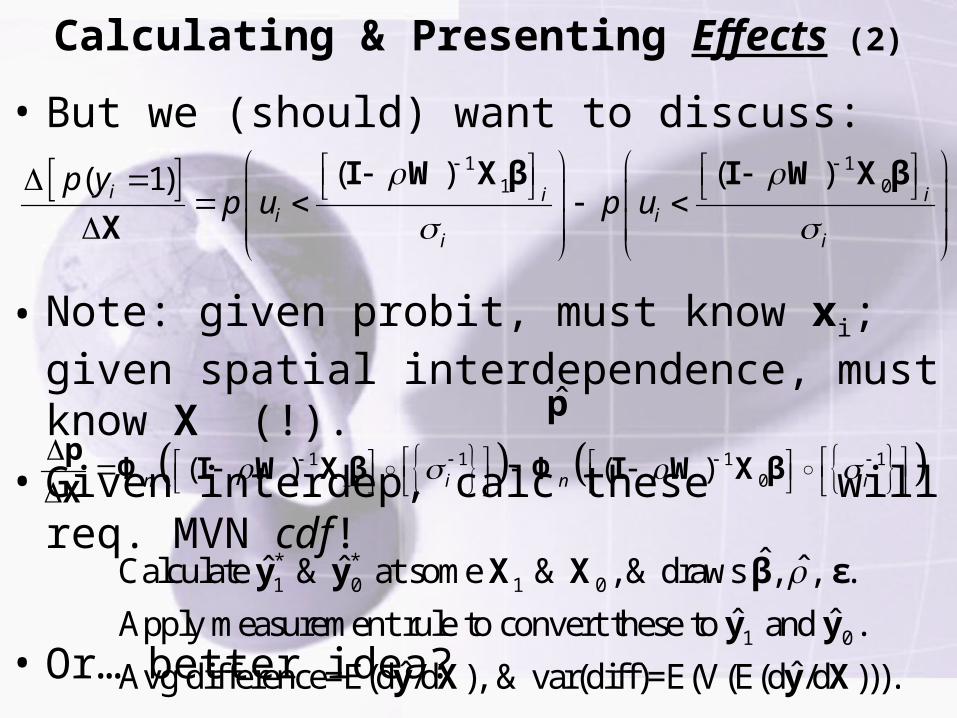
• But we (should) want to discuss:

• Note: given probit, must know xi; given spatial interdependence, must know X (!).

• Given interdep, calc these will req. MVN cdf!

• Or… better idea?

1 11 0( ) ( )( 1)i i i

i ii i

p yp u p u

I W X β I W X β

X

p

1 1 1 11 0( ) ( )n i n i

pΦ I W X β Φ I W X β

X

* *1 0 1 0

1 0

ˆ ˆˆ ˆCalculate & at some & , & draws , , .

ˆ ˆApply measurement rule to convert these to and .

ˆ ˆAvg difference=E(d /d ), & var(diff)=E(V(E(d /d ))).

y y X X β ε

y y

y X y X

An Example Application: US State CHIP Premia

Probit-

ML Probit-MCMC

Spatial-Lag Probit (Gibbs)

Spatial-Error Probit (Gibbs)

Spatial-Lag Probit (RIS)

Constant -4.978 (6.260)

-5.163 (6.292)

-5.606 (10.159)

-5.531 (7.337)

-5.186 (5.944)

Poverty Rate -.244 (.153)

-.265** (.156)

-.374** (.231)

-.243* (.157)

-.171 (.125)

Retail Wage .004

(.003) .004* (.003)

.006* (.004)

.004* (.003)

.004* (.002)

Government Ideology .011

(.013) .011

(.013) .014

(.020) .014

(.014) -.004 (.116)

Inter-party Competition

2.174 (3.388)

2.108 (3.478)

1.473 (6.134)

2.636 (3.794)

1.27 (31.94)

Tax Effort -.014 (.019)

-.014 (.019)

-.020 (.034)

-.017 (.021)

.005 (.017)

Federal Share .045

(.063) .048

(.064) .065

(.095) .043

(.066) .041

(.056) Spatial lag or error-

lag .079

(.798) .102

(.815) .200*** (.148)

.297*** (.196)

.243 (.252)

Pseudo-R2 .222 .220 .607 .574 NA Observations 48 48 48 48 48

Notes: The first two columns’ estimators assume the spatial lags exogenous. The first column gives the standard probit ML estimates. Its parentheses contain estimated standard-errors, and its hypothesis tests assume asymptotic normality of calculated t-statistics. The models in columns two through four apply MCMC methods with diffuse priors, except for a Uniform(0,1) prior on ρ. The reported coefficient estimates are posterior-density means based on 10,000 samples after 1000-sample burn-ins. Parentheses contain sample standard-deviations of these posteriors. The p-values are calculated directly from the posterior density rather than from t-statistics of assumed asymptotic-normality. The last three columns report estimates from true spatial estimators described in the text. In column three, 30 of the 10,000 sampled spatial-lag coefficients were zero; in column four, none of the 10,000 were. Column five reports estimated standard-errors and p-values based on t-statistics assumed asymptotically negative. ***, **, * indicate p-value <.01, <.05, <.10.

Notes: 1. Informative U(0,1) prior on helps. We’ve qualms.

2. Difference in Bayesian vs. frequentist significance also.

3. Note measurement/specification-error seem to have dom’d here for ML.

Example Estimated Spatial Effect, with Certainty Estimate, in Binary-Outcome Model

In lieu of conclusions…• S-QualDep (latent-y*) models hard, doable

•We have a lot of work yet to do:– Illustrate calculation of effects & s.e.’s;

– Explore estimator properties systematically;

– Compare non-spatial probit & spatial-lag ML-probit & approximate specifications

•Next Crucial Extensions:– Extend to other QualDep models…

– Estimated-W models… (see next for a start)

– System-of-Equations in Space…

The m-STAR Model as an Approach to Modeled, Dynamic, Endogenous Interdependence

• Spatial Econometrics and (Political) Economy & Network Analysis and (Political) Sociology

• Co-Evolution Models in Network Analysis– (Node) Behaviors/Attributes & Network (Edges)

• Spatial-Statistical Approaches to Est’d-W

• A Simple Spatial-Econometric Proposal:– Estimated W ≈ Multiple W (m-STAR)– Endogenize W means W(y)=>S-IV in m-STAR

Spatial Econometrics

• Economists & Political Economists

• Core Question:– How alters’ actions affect

ego’s via network & v.v.?– Contagion v. Common

Exposure (Galton’s Problem)• Core Tools:

– SAR, STAR, S-QualDep…– S-GMM, S-ML

Network Analysis

• Sociologists & Political Sociologists

• Core Questions:– How do nets form?– What expl. net struct.?– How ego’s position in net

& net struct affect?• Core Tools

– Net stats (measures), graphics, ERGMs, …

• INTERDEPENDENCE– Definition: yi=f(yj≠i); i’s actions depend on j’s.– Seems subset of “Network Effects”, which also:

• Effects of structure network per se (e.g., # transitive triplets)• Effects of position i in network per se. (e.g., betweenness i)

Where Spatial Econometrics Needs to Go (& Network Analysis is or Needs to Go also)

• Two Things Always Asked Do Next– Qualitative & Limited Dependent Variables

• Bigger estimation challenges because:– Cannot place y itself on RHS, can only place y*.– N-dimensional integration to get probabilities

• Considerable progress: S-Probit/Tobit etc., S-MNP, S-…

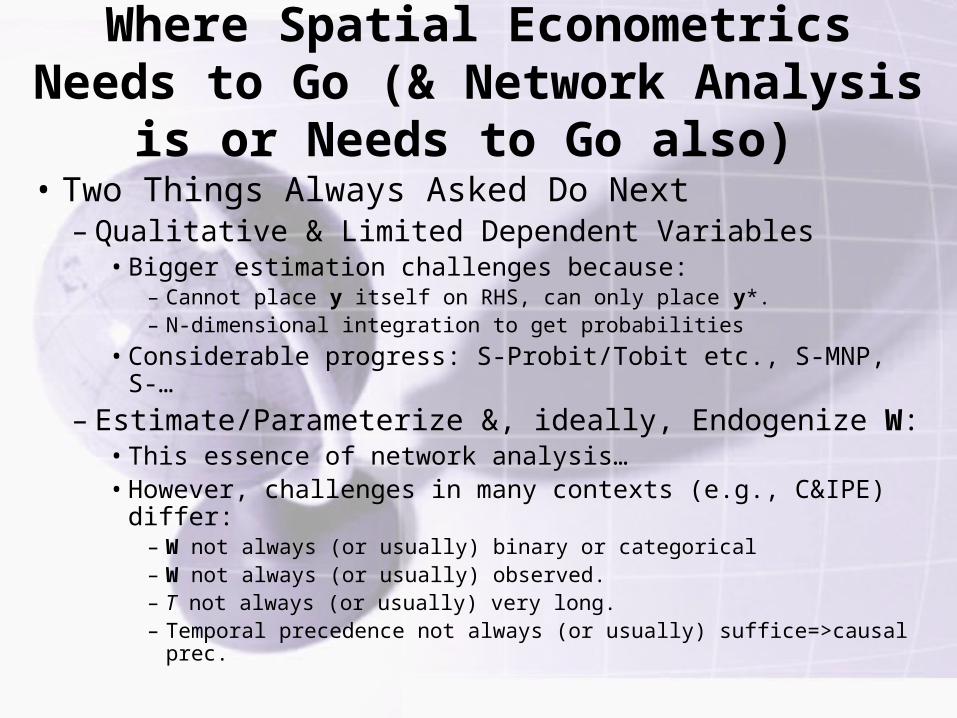
– Estimate/Parameterize &, ideally, Endogenize W:• This essence of network analysis…• However, challenges in many contexts (e.g., C&IPE) differ:

– W not always (or usually) binary or categorical– W not always (or usually) observed.– T not always (or usually) very long.– Temporal precedence not always (or usually) suffice=>causal prec.

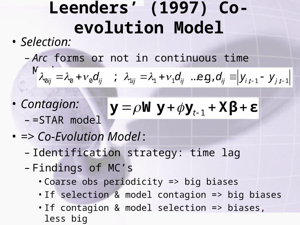
Leenders’ (1997) Co-evolution Model

• Selection:– Arc forms or not in continuous time Markov process:

• Contagion:– =STAR model

• => Co-Evolution Model:– Identification strategy: time lag– Findings of MC’s

• Coarse obs periodicity => big biases

• If selection & model contagion => big biases

• If contagion & model selection => biases, less big

0 0 0 1 1 1 , 1 , 1 ; ...e.g, ij ij ij ij ij i t j td d d y y

1t y Wy y Xβ ε

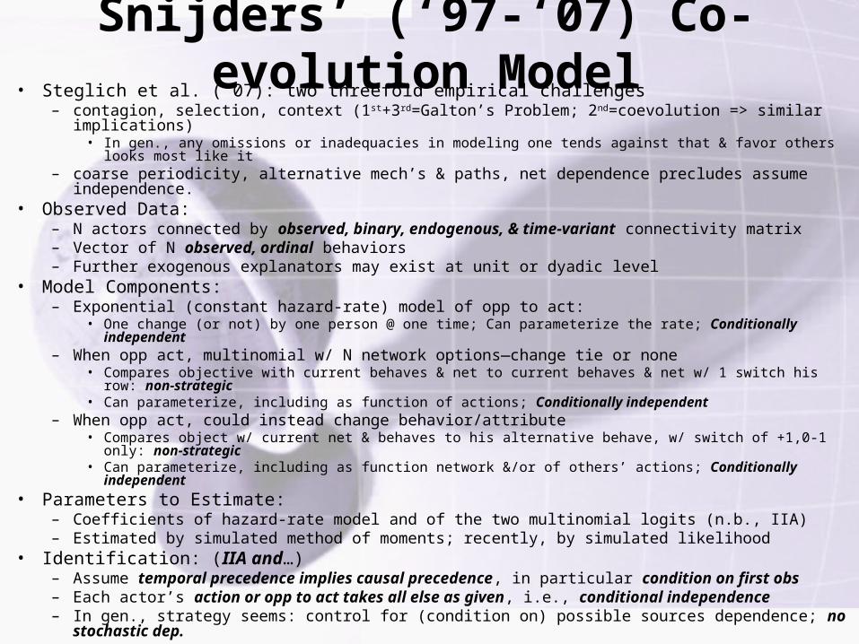
Snijders’ (‘97-‘07) Co-evolution Model• Steglich et al. (‘07): two threefold empirical challenges

– contagion, selection, context (1st+3rd=Galton’s Problem; 2nd=coevolution => similar implications)• In gen., any omissions or inadequacies in modeling one tends against that & favor others looks most like it

– coarse periodicity, alternative mech’s & paths, net dependence precludes assume independence.• Observed Data:

– N actors connected by observed, binary, endogenous, & time-variant connectivity matrix– Vector of N observed, ordinal behaviors– Further exogenous explanators may exist at unit or dyadic level

• Model Components:– Exponential (constant hazard-rate) model of opp to act:

• One change (or not) by one person @ one time; Can parameterize the rate; Conditionally independent– When opp act, multinomial w/ N network options—change tie or none

• Compares objective with current behaves & net to current behaves & net w/ 1 switch his row: non-strategic• Can parameterize, including as function of actions; Conditionally independent

– When opp act, could instead change behavior/attribute• Compares object w/ current net & behaves to his alternative behave, w/ switch of +1,0-1 only: non-

strategic• Can parameterize, including as function network &/or of others’ actions; Conditionally independent

• Parameters to Estimate:– Coefficients of hazard-rate model and of the two multinomial logits (n.b., IIA)– Estimated by simulated method of moments; recently, by simulated likelihood

• Identification: (IIA and…)– Assume temporal precedence implies causal precedence, in particular condition on first obs– Each actor’s action or opp to act takes all else as given, i.e., conditional independence– In gen., strategy seems: control for (condition on) possible sources dependence; no stochastic dep.

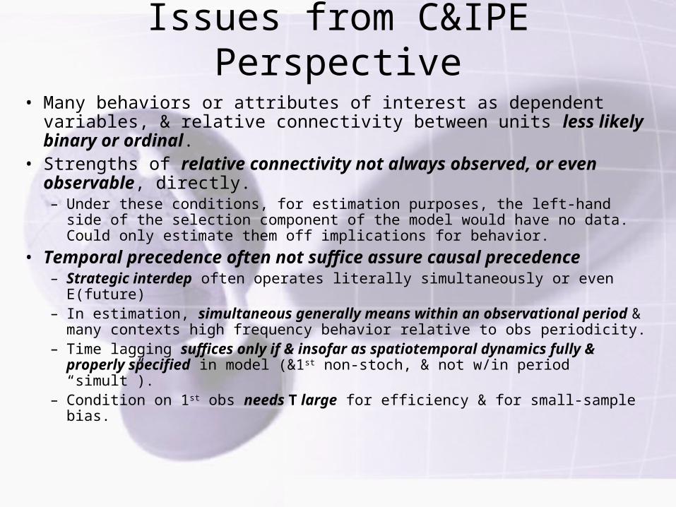
Issues from C&IPE Perspective

• Many behaviors or attributes of interest as dependent variables, & relative connectivity between units less likely binary or ordinal.

• Strengths of relative connectivity not always observed, or even observable, directly.– Under these conditions, for estimation purposes, the left-hand side of the

selection component of the model would have no data. Could only estimate them off implications for behavior.

• Temporal precedence often not suffice assure causal precedence– Strategic interdep often operates literally simultaneously or even E(future)– In estimation, simultaneous generally means within an observational

period & many contexts high frequency behavior relative to obs periodicity.

– Time lagging suffices only if & insofar as spatiotemporal dynamics fully & properly specified in model (&1st non-stoch, & not w/in period “simult”).

– Condition on 1st obs needs T large for efficiency & for small-sample bias.

Multi-Parametric Spatio-Temporal (AR) Lag Model

1

ˆ ˆR

r rr

W W

( , ) ( , ) ( , ) ( , ) ( , ) ( , ) ( , )ˆ1 2 1 2

ˆˆvar( ) ... ...i j i j i j i j i j i j i jR m

ρW W W W Ω W W W

2 /22

1ln ( , , , ; , ) ln(2 ) ln

2NTL e e

ρ β y X A

NT A I W e Ay My Xβ

1 1 2 2

1

...

, where

R R

R

r rr

y W y W y W y My Xβ ε

Wy My Xβ ε W W

1 21 2 , 1

1 21 2

...

...

R ii ij j ij j R ij j i t k k i

j j j k

R iij ij R ij j k k i

j k

R iR ij j k k i

j r k

y w y w y w y y x

w w w y x

w y x

Co-Evolution Models in m-STAR Format

• Wr = covariates expected explain network• Co-evolution models=models with W=f(y): larger challenges.

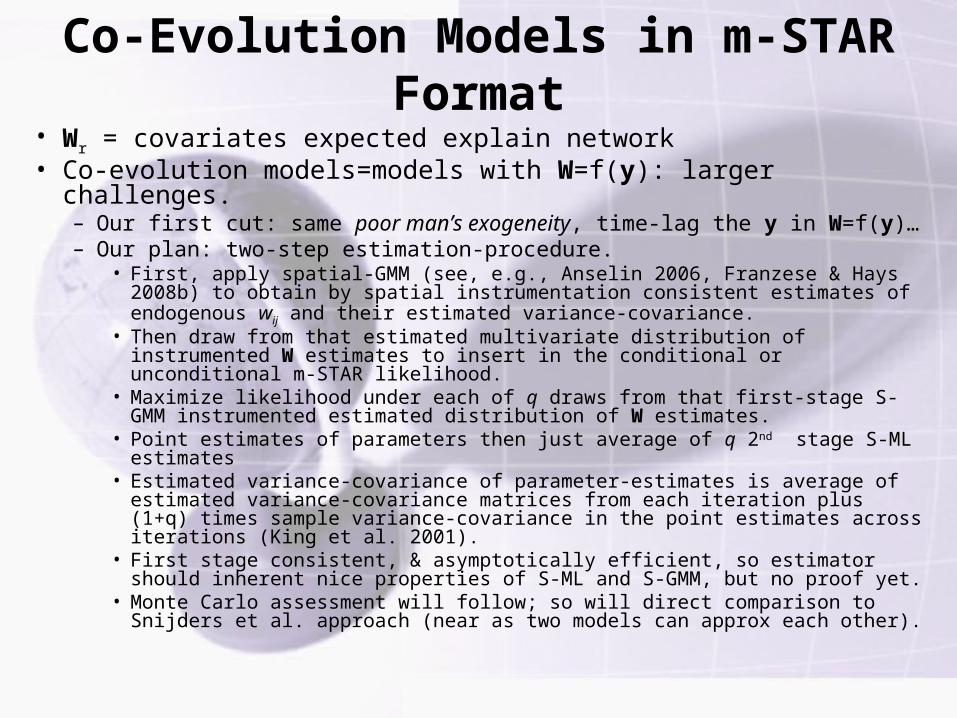
– Our first cut: same poor man’s exogeneity, time-lag the y in W=f(y)…– Our plan: two-step estimation-procedure.

• First, apply spatial-GMM (see, e.g., Anselin 2006, Franzese & Hays 2008b) to obtain by spatial instrumentation consistent estimates of endogenous wij and their estimated variance-covariance.

• Then draw from that estimated multivariate distribution of instrumented W estimates to insert in the conditional or unconditional m-STAR likelihood.

• Maximize likelihood under each of q draws from that first-stage S-GMM instrumented estimated distribution of W estimates.

• Point estimates of parameters then just average of q 2nd stage S-ML estimates• Estimated variance-covariance of parameter-estimates is average of estimated

variance-covariance matrices from each iteration plus (1+q) times sample variance-covariance in the point estimates across iterations (King et al. 2001).

• First stage consistent, & asymptotically efficient, so estimator should inherent nice properties of S-ML and S-GMM, but no proof yet.

• Monte Carlo assessment will follow; so will direct comparison to Snijders et al. approach (near as two models can approx each other).

Active Labor Market Program Expenditures in OECD Countries, 1981-2002Dependent variable

(1) (2) (3) (4) (5) (6) (7) (8) (9)Temporal Lag 0.875*** 0.880*** 0.892*** 0.872*** 0.873*** 0.865*** 0.830*** 0.833*** 0.822***

(0.028) (0.026) (0.026) (0.029) (0.028) (0.028) (0.035) (0.034) (0.034)Real GDP Growth Rate 1.365*** 1.339*** -0.032 0.269 0.312 -0.445 0.036 0.040 -0.890

(0.430) (0.423) (1.105) (0.210) (0.204) (0.640) (0.196) (0.189) (0.620)Standerdized Unem. Rate -0.070 -0.074 -0.338 0.361 0.412 0.452 -0.169 -0.187 -0.580

(0.826) (0.794) (0.867) (0.465) (0.445) (0.508) (0.457) (0.438) (0.491)Union Density 0.888*** 0.918*** 0.814*** 0.205 0.205 0.161 0.567*** 0.584*** 0.575***

(0.315) (0.303) (0.302) (0.174) (0.167) (0.171) (0.176) (0.168) (0.173)Deindustrialization 1.259 1.249 0.771 0.106 0.114 -0.220 1.4260*** 1.413*** 1.100**

(0.820) (0.783) (0.776) (0.469) (0.448) (0.454) (0.455) (0.437) (0.442)Trade Openness -0.522*** -0.484*** -0.307 -0.187 -0.168* -0.037 0.018 0.022 0.064

(0.176) (0.169) (0.196) (0.101) (0.097) (0.114) (0.108) (0.103) (0.120)Working Age Population 0.946 0.916 0.090 2.239** 2.210*** 1.819** -0.139 -0.140 -0.366

(1.561) (1.497) (1.571) (0.888) (0.861) (0.925) (0.866) (0.828) (0.885)Left Cabinet Seats -0.024 -0.016 -0.015 0.035 0.036 0.042* -0.049** -0.046** -0.040

(0.041) (0.039) (0.038) (0.023) (0.022) (0.022) (0.023) (0.022) (0.021)Christian Dem. Cabinet Seats -0.160 -0.173* -0.146 -0.070 -0.074 -0.056 -0.032 -0.036 -0.019

(0.099) (0.095) (0.092) (0.056) (0.054) (0.054) (0.055) (0.052) (0.052)Left Libertarian Vote -0.285 -0.293 -0.421 -0.316 -0.325 -0.399 -0.248 -0.241 -0.274

(0.650) (0.621) (0.603) (0.371) (0.354) (0.028) (0.361) (0.345) (0.342)

Spatial Weights:Borders -0.004 -0.006 -0.007 -0.008 0.001 -0.002

(0.007) (0.007) (0.007) (0.007) (0.007) (0.007)

European Union Membership -0.033*** -0.032*** -0.033*** -0.033*** -0.036*** -0.035***(0.012) (0.012) (0.012) (0.012) (0.013) (0.013)

Trade Shares 0.018 0.025 0.027 0.030* 0.004 0.013(0.017) (0.018) (0.017) (0.018) (0.017) (0.017)

ALM Program Expenditures 0.008 -0.004 -0.009 -0.015 0.019 0.005(0.016) (0.017) (0.015) (0.016) (0.015) (0.016)

22.176 21.184*** 19.960*** 12.604 12.028*** 11.664*** 12.324 11.765*** 11.328***(0.785) (0.739) (0.452) (0.436) (0.436) (0.419)

Log-Likelihood -1646.410 -1642.34 -1620.8 -1438.49 -1434.31 -1423.27 -1430.23 -1425.92 -1411.92

NoteAll regressions include fixed country effects. In addition to the country fixed effects, Model (3), (6) and (9) also include fixed year effects.All the spatial weights matrices are row-standardized.The parentheses contain standard errors.*** Significant at the .01 level; ** Significant at the .05 level; * Significant at the .10 level.

Total ALM LMT SEMP

Table 3: First-Period Spatial Effects of Union Density on Logged LMT per Capita (2000 PPP$) AUS AUT BEL CAN DNK FIN FRA GER GRC IRE ITA JPN NTH NWZ NOR PRT ESP SWE CHE GBR USA

AUS 58.4*** 0.03 0.21 0.02 0.05 0.09 0.11 0.1 0 0.13 0.07* 0.09 0.05* 0.08 0.01 0.02** 0.11 0.08 0.04* 0.02 0.06(16.83) (0.03) (0.17) (0.02) (0.04) (0.07) (0.08) (0.07) (0) (0.11) (0.04) (0.31) (0.03) (0.33) (0) (0.01) (0.09) (0.06) (0.03) (0.08) (0.25)

AUT 0.03 58.4*** 0.05 0.01 -0.1* -0.07 -0.04 0.05 -0.16** -0.03 -0.06 0.03 -0.11* 0.02 0.01 -0.14** -0.05 -0.08 0.07 -0.15** 0.02(0.02) (16.83) (0.14) (0.01) (0.06) (0.07) (0.06) (0.34) (0.07) (0.1) (0.09) (0.02) (0.06) (0.02) (0) (0.07) (0.08) (0.06) (0.1) (0.07) (0.05)

BEL 0.04 -0.12** 58.4** 0.01 -0.09 -0.05 0.02 0 -0.16** 0 -0.07 0.03 -0.06 0.02 0.01 -0.13 -0.03 -0.06 0.06 -0.12 0.02(0.03) (0.06) (16.83) (0.01) (0.07) (0.08) (0.09) (0.11) (0.07) (0.11) (0.06) (0.02) (0.09) (0.02) (0.01) (0.06) (0.08) (0.07) (0.04) (0.08) (0.07)

CAN 0.03 0.03 0.21 58.4** 0.05 0.09 0.11 0.09 0 0.13 0.06 0.03 0.04 0.02 0.01 0.02** 0.11 0.08 0.05 0.01 0.23(0.02) (0.03) (0.17) (16.83) (0.04) (0.07) (0.08) (0.06) (0) (0.11) (0.05) (0.05) (0.03) (0.02) (0.01) (0.01) (0.09) (0.06) (0.04) (0.03) (0.58)

DNK 0.03 -0.12 0.06 0.01 58.4** -0.06 -0.04 0.01 -0.16** -0.02 -0.09 0.03 -0.1 0.02 0.02 -0.14** -0.05 -0.03 0.05* -0.13 0.02(0.02) (0.06) (0.14) (0.01) (16.83) (0.06) (0.06) (0.12) (0.07) (0.1) (0.06) (0.03) (0.07) (0.02) (0.06) (0.07) (0.08) (0.13) (0.03) (0.12) (0.06)

FIN 0.04 -0.12** 0.06 0.01 -0.09 58.4** -0.03 -0.03 -0.16** -0.02 -0.08 0.03 -0.1* 0.02 0.04 -0.14** -0.04 -0.02 0.05* -0.13 0.03(0.02) (0.06) (0.14) (0.01) (0.06) (16.83) (0.07) (0.14) (0.07) (0.1) (0.06) (0.04) (0.06) (0.02) (0.16) (0.07) (0.08) (0.12) (0.03) (0.12) (0.09)

FRA 0.03** -0.12** 0.09 0.01 -0.1* -0.06 58.4** -0.01 -0.16** -0.02 -0.06 0.03 -0.1* 0.02 0.01 -0.14** -0.02 -0.07 0.06 -0.12 0.03(0.03) (0.06) (0.13) (0.01) (0.06) (0.08) (16.83) (0.12) (0.07) (0.1) (0.07) (0.03) (0.06) (0.02) (0.01) (0.06) (0.07) (0.07) (0.06) (0.08) (0.09)

GER 0.03 -0.1* 0.08 0.01 -0.09 -0.06 -0.01 58.4** -0.16** -0.02 -0.07 0.03 -0.08 0.02 0.01 -0.14** -0.04 -0.07 0.07 -0.13 0.03(0.02) (0.06) (0.14) (0.01) (0.09) (0.07) (0.07) (16.83) (0.07) (0.1) (0.08) (0.04) (0.06) (0.02) (0.02) (0.06) (0.07) (0.06) (0.05) (0.11) (0.1)

GRC 0.03 -0.12** 0.05 0.01 -0.1* -0.07 -0.03 -0.02 58.4** -0.03 -0.06 0.03 -0.1 0.02 0.01 -0.14** -0.05 -0.08 0.05* -0.14 0.02(0.02) (0.06) (0.13) (0.01) (0.06) (0.07) (0.07) (0.19) (16.83) (0.1) (0.06) (0.04) (0.07) (0.02) (0) (0.07) (0.07) (0.06) (0.03) (0.09) (0.06)

IRE 0.04 -0.12** 0.08 0.01 -0.1* -0.06 -0.03 -0.04 -0.16** 58.4** -0.08 0.03 -0.1* 0.02 0.01 -0.14** -0.04 -0.07 0.05 -0.03 0.04(0.03) (0.06) (0.14) (0.01) (0.06) (0.08) (0.07) (0.08) (0.07) (16.83) (0.06) (0.04) (0.06) (0.02) (0.01) (0.07) (0.08) (0.07) (0.04) (0.23) (0.160

ITA 0.03 -0.1 0.06 0.01 -0.1* -0.07 0 -0.02 -0.16** -0.02 58.4** 0.03 -0.1 0.02 0.01 -0.14** -0.04 -0.08 0.07 -0.14 0.03(0.02) (0.13) (0.13) (0.01) (0.06) (0.08) (0.08) (0.2) (0.07) (0.1) (16.83) (0.02) (0.06) (0.02) (0.01) (0.06) (0.06) (0.06) (0.11) (0.1) (0.09)

JPN 0.05 0.03 0.21 0.02 0.05 0.09 0.11 0.11 0 0.13 0.07* 58.4** 0.05* 0.02 0.01 0.02** 0.11 0.08 0.05* 0.01 0.12(0.06) (0.02) (0.17) (0.05) (0.04) (0.07) (0.08) (0.08) (0) (0.11) (0.04) (16.83) (0.03) (0.02) (0.01) (0.01) (0.09) (0.06) (0.03) (0.06) (0.53)

NTH 0.03 -0.12** 0.1 0.01 -0.1* -0.07 -0.03 0.01 -0.16** -0.02 -0.09 0.03 58.4** 0.02 0.01 -0.14** -0.04 -0.08 0.05* -0.12 0.02(0.02) (0.06) (0.13) (0.01) (0.06) (0.07) (0.08) (0.16) (0.07) (0.1) (0.06) (0.02) (16.83) (0.02) (0.01) (0.07) (0.07) (0.06) (0.03) (0.09) (0.07)

NWZ 0.14 0.03 0.21 0.02 0.05 0.09 0.11 0.1* 0 0.13 0.07* 0.07 0.04 58.4** 0.01 0.02** 0.11 0.08 0.05 0.02 0.05(0.24) (0.03) (0.17) (0.02) (0.04) (0.07) (0.08) (0.06) (0) (0.11) (0.04) (0.19) (0.03) (16.83) (0) (0.01) (0.09) (0.06) (0.04) (0.08) (0.21)

NOR 0.03 0.03 0.21 0.02 0.06 0.12 0.12 0.12 0 0.13 0.07* 0.03 0.06 0.02 58.4** 0.02** 0.11 0.13 0.05* 0.05 0.02(0.03) (0.02) (0.16) (0.03) (0.05) (0.2) (0.08) (0.13) (0) (0.1) (0.04) (0.03) (0.07) (0.02) (16.83) (0.01) (0.08) (0.13) (0.03) (0.2) (0.08)

PRT 0.03 -0.12** 0.05 0.01 -0.1* -0.07 -0.02 -0.03 -0.16** -0.03 -0.08 0.03 -0.11* 0.02 0.01 58.4** 0.04 -0.08 0.05* -0.13 0.02(0.02) (0.06) (0.13) (0.01) (0.06) (0.07) (0.1) (0.14) (0.07) (0.1) (0.06) (0.02) (0.06) (0.02) (0.01) (16.83) (0.27) (0.06) (0.03) (0.11) (0.05)

ESP 0.03 -0.12** 0.07 0.01 -0.1* -0.06 0.03 -0.03 -0.16** -0.02 -0.07 0.03 -0.1* 0.02 0.01 -0.1 58.4** -0.07 0.05 -0.13 0.02(0.03) (0.06) (0.14) (0.01) (0.06) (0.08) (0.11) (0.14) (0.07) (0.1) (0.09) (0.03) (0.06) (0.02) (0.01) (0.16) (16.83) (0.07) (0.03) (0.11) (0.08)

SWE 0.03 -0.12** 0.06 0.01 -0.07 -0.04 -0.04 -0.03 -0.16** -0.02 -0.09 0.03 -0.1 0.02 0.04 -0.14** -0.04 58.4** 0.05* -0.13 0.03(0.02) (0.06) (0.14) (0.01) (0.1) (0.12) (0.06) (0.14) (0.07) (0.1) (0.06) (0.03) (0.07) (0.02) (0.08) (0.07) (0.08) (16.83) (0.03) (0.12) (0.09)

CHE 0.03 0.05 0.22 0.01 0.06 0.09 0.15* 0.17 0 0.14 0.1 0.03 0.05 0.02 0.01 0.02** 0.11 0.08 58.4** 0.02 0.03(0.02) (0.08) (0.16) (0.01) (0.04) (0.07) (0.09) (0.22) (0.01) (0.11) (0.07) (0.04) (0.04) (0.02) (0) (0.01) (0.08) (0.06) (16.83) (0.07) (0.1)

GBR 0.03 -0.12** 0.07 0.01 -0.1* -0.07 -0.02 -0.04 -0.16** -0.01 -0.09 0.03 -0.09 0.02 0.01 -0.14** -0.05 -0.08 0.05* 58.4** 0.04(0.02) (0.06) (0.16) (0.02) (0.06) (0.07) (0.07) (0.13) (0.07) (0.11) (0.06) (0.04) (0.07) (0.01) (0.02) (0.07) (0.07) (0.06) (0.03) (16.83) (0.16)

USA 0.04** 0.03 0.21 0.13 0.05 0.09 0.11 0.1 0 0.13 0.07* 0.07 0.05* 0.02 0.01 0.02** 0.11 0.08 0.05* 0.02 58.4**(0.02) (0.02) (0.16) (0.24) (0.04) (0.07) (0.07) (0.08) (0) (0.1) (0.04) (0.21) (0.03) (0.02) (0.01) (0.01) (0.08) (0.06) (0.03) (0.08) (16.83)

Notes: The cells report the first-period spatial effect of a 1% increase in the column country’s union density on its own subsidized employment expenditures ( 100) and the expenditures ( 100) of its OECD counterparts (identified by the rows) based on the model (8) estimates.

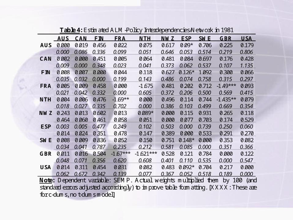
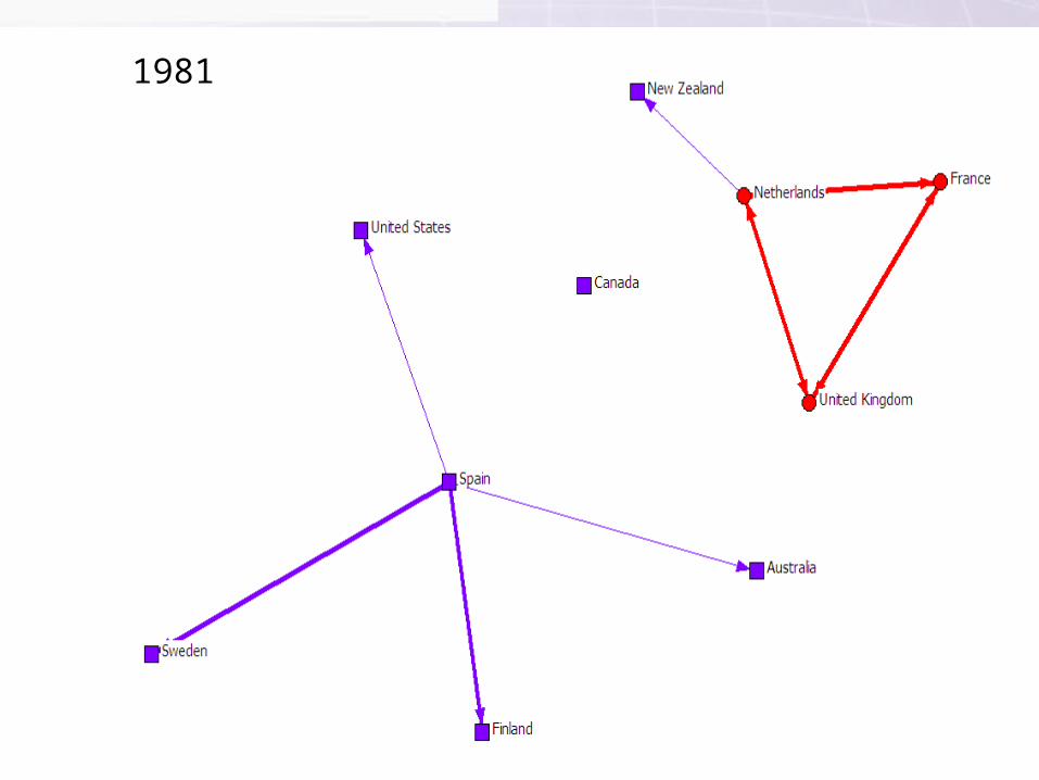
Table 4: Estimated ALM-Policy Interdependencies/Network in 1981 AUS CAN FIN FRA NTH NWZ ESP SWE GBR USA

AUS 0.000 0.019 0.456 0.022 0.075 0.617 0.09* 0.706 0.225 0.1790.000 0.086 0.336 0.099 0.051 0.646 0.053 0.514 0.219 0.806

CAN 0.002 0.000 0.451 0.005 0.064 0.481 0.084 0.697 0.176 0.4280.009 0.000 0.348 0.023 0.041 0.373 0.062 0.537 0.107 1.135

FIN 0.008 0.007 0.000 0.044 0.118 0.627 0.126* 1.092 0.300 0.0660.035 0.032 0.000 0.199 0.143 0.486 0.074 0.758 0.315 0.297

FRA 0.005 0.009 0.458 0.000 -1.675 0.481 0.202 0.712 -1.49*** 0.0930.021 0.042 0.332 0.000 0.605 0.372 0.206 0.500 0.569 0.415

NTH 0.004 0.006 0.476 -1.69** 0.000 0.496 0.114 0.744 -1.435** 0.0790.018 0.027 0.335 0.702 0.000 0.386 0.103 0.499 0.669 0.354

NWZ 0.243 0.013 0.602 0.013 0.089* 0.000 0.115 0.931 0.265 0.1180.464 0.060 0.461 0.058 0.051 0.000 0.077 0.703 0.174 0.529

ESP 0.003 0.005 0.477 0.249 0.102 0.503 0.000 0.739 0.250 0.0600.014 0.024 0.351 0.478 0.147 0.389 0.000 0.533 0.291 0.270

SWE 0.008 0.009 0.836 0.052 0.150 0.751 0.148* 0.000 0.353 0.0820.034 0.041 0.787 0.235 0.212 0.581 0.085 0.000 0.351 0.366

GBR 0.011 0.016 0.504 -1.67*** -1.621*** 0.528 0.121 0.784 0.000 0.1220.048 0.071 0.356 0.620 0.608 0.401 0.110 0.535 0.000 0.547

USA 0.014 0.311 0.454 0.031 0.082 0.483 0.092* 0.704 0.217 0.0000.062 0.672 0.342 0.139 0.077 0.367 0.052 0.518 0.189 0.000

Note: Dependent variable: SEMP. Actual weights multiplied them by 100 (and standard errors adjusted accordingly) to improve table formatting. [XXXX: These are for c-dums, no t-dums model]

1981

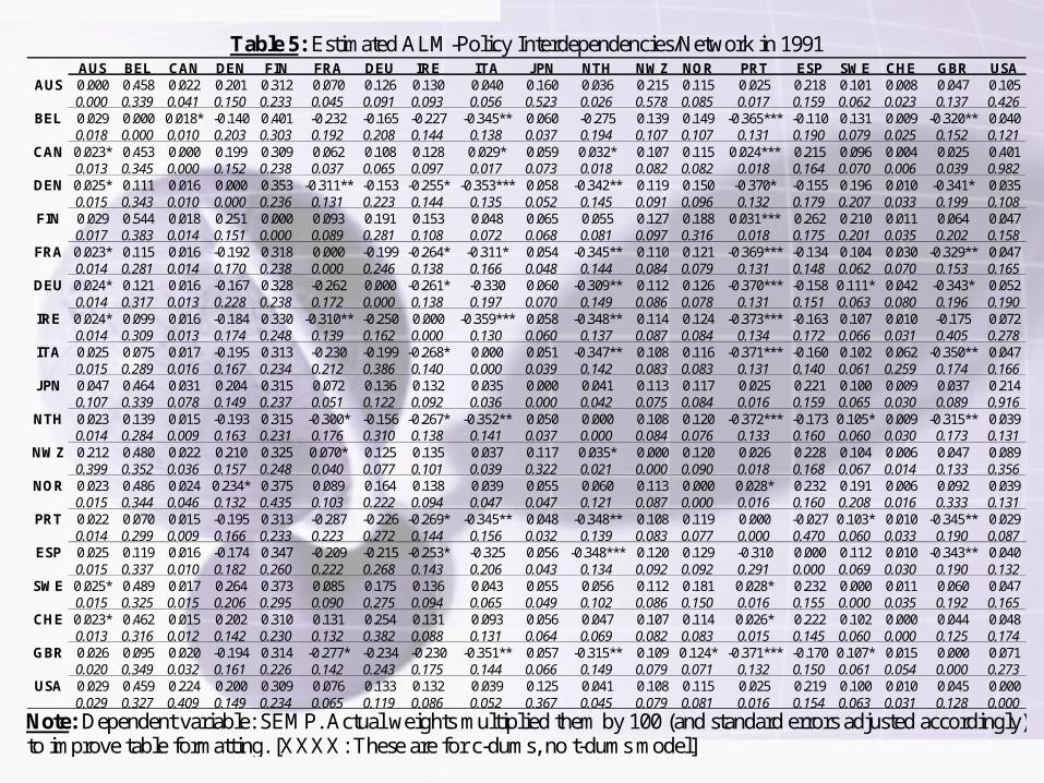
Table 5: Estimated ALM-Policy Interdependencies/Network in 1991 AUS BEL CAN DEN FIN FRA DEU IRE ITA JPN NTH NWZ NOR PRT ESP SWE CHE GBR USA

AUS 0.000 0.458 0.022 0.201 0.312 0.070 0.126 0.130 0.040 0.160 0.036 0.215 0.115 0.025 0.218 0.101 0.008 0.047 0.1050.000 0.339 0.041 0.150 0.233 0.045 0.091 0.093 0.056 0.523 0.026 0.578 0.085 0.017 0.159 0.062 0.023 0.137 0.426

BEL 0.029 0.000 0.018* -0.140 0.401 -0.232 -0.165 -0.227 -0.345** 0.060 -0.275 0.139 0.149 -0.365*** -0.110 0.131 0.009 -0.320** 0.0400.018 0.000 0.010 0.203 0.303 0.192 0.208 0.144 0.138 0.037 0.194 0.107 0.107 0.131 0.190 0.079 0.025 0.152 0.121

CAN 0.023* 0.453 0.000 0.199 0.309 0.062 0.108 0.128 0.029* 0.059 0.032* 0.107 0.115 0.024*** 0.215 0.096 0.004 0.025 0.4010.013 0.345 0.000 0.152 0.238 0.037 0.065 0.097 0.017 0.073 0.018 0.082 0.082 0.018 0.164 0.070 0.006 0.039 0.982

DEN 0.025* 0.111 0.016 0.000 0.353 -0.311** -0.153 -0.255* -0.353*** 0.058 -0.342** 0.119 0.150 -0.370* -0.155 0.196 0.010 -0.341* 0.0350.015 0.343 0.010 0.000 0.236 0.131 0.223 0.144 0.135 0.052 0.145 0.091 0.096 0.132 0.179 0.207 0.033 0.199 0.108

FIN 0.029 0.544 0.018 0.251 0.000 0.093 0.191 0.153 0.048 0.065 0.055 0.127 0.188 0.031*** 0.262 0.210 0.011 0.064 0.0470.017 0.383 0.014 0.151 0.000 0.089 0.281 0.108 0.072 0.068 0.081 0.097 0.316 0.018 0.175 0.201 0.035 0.202 0.158

FRA 0.023* 0.115 0.016 -0.192 0.318 0.000 -0.199 -0.264* -0.311* 0.054 -0.345** 0.110 0.121 -0.369*** -0.134 0.104 0.030 -0.329** 0.0470.014 0.281 0.014 0.170 0.238 0.000 0.246 0.138 0.166 0.048 0.144 0.084 0.079 0.131 0.148 0.062 0.070 0.153 0.165

DEU 0.024* 0.121 0.016 -0.167 0.328 -0.262 0.000 -0.261* -0.330 0.060 -0.309** 0.112 0.126 -0.370*** -0.158 0.111* 0.042 -0.343* 0.0520.014 0.317 0.013 0.228 0.238 0.172 0.000 0.138 0.197 0.070 0.149 0.086 0.078 0.131 0.151 0.063 0.080 0.196 0.190

IRE 0.024* 0.099 0.016 -0.184 0.330 -0.310** -0.250 0.000 -0.359*** 0.058 -0.348** 0.114 0.124 -0.373*** -0.163 0.107 0.010 -0.175 0.0720.014 0.309 0.013 0.174 0.248 0.139 0.162 0.000 0.130 0.060 0.137 0.087 0.084 0.134 0.172 0.066 0.031 0.405 0.278

ITA 0.025 0.075 0.017 -0.195 0.313 -0.230 -0.199 -0.268* 0.000 0.051 -0.347** 0.108 0.116 -0.371*** -0.160 0.102 0.062 -0.350** 0.0470.015 0.289 0.016 0.167 0.234 0.212 0.386 0.140 0.000 0.039 0.142 0.083 0.083 0.131 0.140 0.061 0.259 0.174 0.166

JPN 0.047 0.464 0.031 0.204 0.315 0.072 0.136 0.132 0.035 0.000 0.041 0.113 0.117 0.025 0.221 0.100 0.009 0.037 0.2140.107 0.339 0.078 0.149 0.237 0.051 0.122 0.092 0.036 0.000 0.042 0.075 0.084 0.016 0.159 0.065 0.030 0.089 0.916

NTH 0.023 0.139 0.015 -0.193 0.315 -0.300* -0.156 -0.267* -0.352** 0.050 0.000 0.108 0.120 -0.372*** -0.173 0.105* 0.009 -0.315** 0.0390.014 0.284 0.009 0.163 0.231 0.176 0.310 0.138 0.141 0.037 0.000 0.084 0.076 0.133 0.160 0.060 0.030 0.173 0.131

NWZ 0.212 0.480 0.022 0.210 0.325 0.070* 0.125 0.135 0.037 0.117 0.035* 0.000 0.120 0.026 0.228 0.104 0.006 0.047 0.0890.399 0.352 0.036 0.157 0.248 0.040 0.077 0.101 0.039 0.322 0.021 0.000 0.090 0.018 0.168 0.067 0.014 0.133 0.356

NOR 0.023 0.486 0.024 0.234* 0.375 0.089 0.164 0.138 0.039 0.055 0.060 0.113 0.000 0.028* 0.232 0.191 0.006 0.092 0.0390.015 0.344 0.046 0.132 0.435 0.103 0.222 0.094 0.047 0.047 0.121 0.087 0.000 0.016 0.160 0.208 0.016 0.333 0.131

PRT 0.022 0.070 0.015 -0.195 0.313 -0.287 -0.226 -0.269* -0.345** 0.048 -0.348** 0.108 0.119 0.000 -0.027 0.103* 0.010 -0.345** 0.0290.014 0.299 0.009 0.166 0.233 0.223 0.272 0.144 0.156 0.032 0.139 0.083 0.077 0.000 0.470 0.060 0.033 0.190 0.087

ESP 0.025 0.119 0.016 -0.174 0.347 -0.209 -0.215 -0.253* -0.325 0.056 -0.348*** 0.120 0.129 -0.310 0.000 0.112 0.010 -0.343** 0.0400.015 0.337 0.010 0.182 0.260 0.222 0.268 0.143 0.206 0.043 0.134 0.092 0.092 0.291 0.000 0.069 0.030 0.190 0.132

SWE 0.025* 0.489 0.017 0.264 0.373 0.085 0.175 0.136 0.043 0.055 0.056 0.112 0.181 0.028* 0.232 0.000 0.011 0.060 0.0470.015 0.325 0.015 0.206 0.295 0.090 0.275 0.094 0.065 0.049 0.102 0.086 0.150 0.016 0.155 0.000 0.035 0.192 0.165

CHE 0.023* 0.462 0.015 0.202 0.310 0.131 0.254 0.131 0.093 0.056 0.047 0.107 0.114 0.026* 0.222 0.102 0.000 0.044 0.0480.013 0.316 0.012 0.142 0.230 0.132 0.382 0.088 0.131 0.064 0.069 0.082 0.083 0.015 0.145 0.060 0.000 0.125 0.174

GBR 0.026 0.095 0.020 -0.194 0.314 -0.277* -0.234 -0.230 -0.351** 0.057 -0.315** 0.109 0.124* -0.371*** -0.170 0.107* 0.015 0.000 0.0710.020 0.349 0.032 0.161 0.226 0.142 0.243 0.175 0.144 0.066 0.149 0.079 0.071 0.132 0.150 0.061 0.054 0.000 0.273

USA 0.029 0.459 0.224 0.200 0.309 0.076 0.133 0.132 0.039 0.125 0.041 0.108 0.115 0.025 0.219 0.100 0.010 0.045 0.0000.029 0.327 0.409 0.149 0.234 0.065 0.119 0.086 0.052 0.367 0.045 0.079 0.081 0.016 0.154 0.063 0.031 0.128 0.000

Note: Dependent variable: SEMP. Actual weights multiplied them by 100 (and standard errors adjusted accordingly) to improve table formatting. [XXXX: These are for c-dums, no t-dums model]

1991

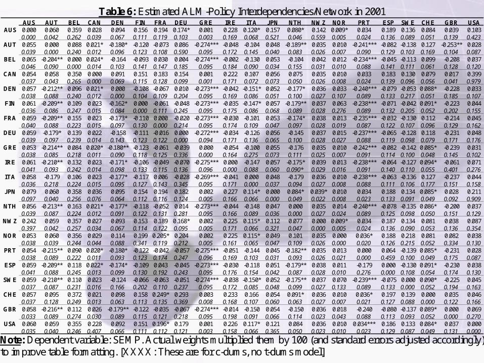
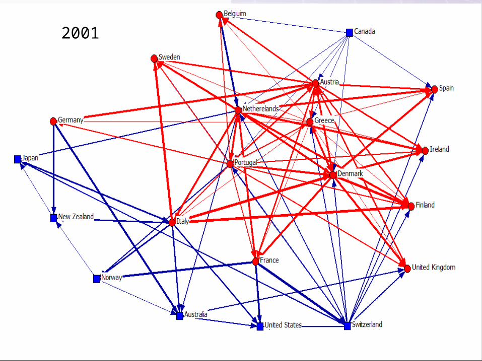
Table 6: Estimated ALM-Policy Interdependencies/Network in 2001 AUS AUT BEL CAN DEN FIN FRA DEU GRE IRE ITA JPN NTH NWZ NOR PRT ESP SWE CHE GBR USA

AUS 0.000 0.060 0.359 0.028 0.094 0.156 0.194 0.174* 0.001 0.228 0.120* 0.157 0.080* 0.142 0.009* 0.034 0.189 0.136 0.084 0.039 0.1030.000 0.042 0.262 0.039 0.067 0.111 0.119 0.103 0.003 0.169 0.068 0.521 0.046 0.559 0.005 0.024 0.136 0.089 0.051 0.139 0.423

AUT 0.055 0.000 0.088 0.021* -0.180* -0.120 -0.073 0.086 -0.274*** -0.048 -0.104 0.048 -0.189** 0.035 0.010 -0.241*** -0.082 -0.138 0.127 -0.253** 0.0280.039 0.000 0.240 0.012 0.096 0.123 0.108 0.590 0.095 0.172 0.145 0.040 0.083 0.026 0.007 0.090 0.129 0.103 0.169 0.104 0.087

BEL 0.065 -0.204** 0.000 0.024* -0.164 -0.093 0.030 0.004 -0.274*** -0.002 -0.130 0.053 -0.104 0.042 0.012 -0.234*** -0.045 -0.113 0.099 -0.208 0.0370.046 0.090 0.000 0.014 0.103 0.141 0.147 0.185 0.095 0.184 0.090 0.034 0.155 0.031 0.010 0.088 0.141 0.111 0.061 0.128 0.120

CAN 0.054 0.058 0.350 0.000 0.091 0.151 0.183 0.154 0.001 0.222 0.107 0.056 0.075 0.035 0.010 0.033 0.183 0.130 0.079 0.017 0.3990.037 0.043 0.265 0.000 0.069 0.115 0.128 0.099 0.001 0.171 0.072 0.073 0.050 0.026 0.008 0.024 0.139 0.096 0.056 0.041 0.979

DEN 0.057 -0.212** 0.096 0.021* 0.000 -0.108 -0.067 0.010 -0.273*** -0.042 -0.151* 0.052 -0.177* 0.036 0.033 -0.240*** -0.079 -0.053 0.088* -0.228 0.0330.038 0.088 0.240 0.012 0.000 0.104 0.109 0.204 0.095 0.169 0.086 0.051 0.100 0.027 0.107 0.089 0.133 0.217 0.051 0.185 0.107

FIN 0.061 -0.209** 0.109 0.023 -0.162* 0.000 -0.061 -0.048 -0.273*** -0.035 -0.147* 0.057 -0.179** 0.037 0.063 -0.238*** -0.071 -0.042 0.091* -0.223 0.0440.036 0.086 0.247 0.015 0.084 0.000 0.111 0.245 0.095 0.175 0.086 0.068 0.089 0.028 0.276 0.089 0.132 0.205 0.052 0.202 0.155

FRA 0.059 -0.209** 0.155 0.023 -0.173* -0.110 0.000 -0.020 -0.273*** -0.030 -0.101 0.053 -0.174* 0.038 0.013 -0.235*** -0.032 -0.130 0.112 -0.214 0.0450.040 0.088 0.223 0.015 0.097 0.130 0.000 0.214 0.095 0.174 0.109 0.047 0.097 0.028 0.019 0.087 0.122 0.107 0.096 0.129 0.162

DEU 0.059 -0.179* 0.139 0.022 -0.158 -0.111 -0.016 0.000 -0.272*** -0.034 -0.126 0.056 -0.145 0.037 0.015 -0.237*** -0.065 -0.128 0.118 -0.231 0.0480.039 0.097 0.239 0.014 0.143 0.123 0.122 0.000 0.094 0.171 0.136 0.065 0.100 0.028 0.027 0.088 0.119 0.098 0.079 0.171 0.176

GRE 0.053 -0.214** 0.084 0.020* -0.180** -0.123 -0.061 -0.039 0.000 -0.054 -0.100 0.055 -0.176 0.035 0.010 -0.242*** -0.082 -0.142 0.085* -0.239 0.0310.038 0.085 0.218 0.011 0.090 0.118 0.125 0.336 0.000 0.164 0.275 0.073 0.111 0.025 0.007 0.091 0.114 0.100 0.048 0.145 0.102

IRE 0.061 -0.210** 0.132 0.023 -0.171* -0.106 -0.049 -0.070 -0.275*** 0.000 -0.147 0.057 -0.175* 0.039 0.013 -0.238*** -0.064 -0.127 0.094* -0.061 0.0710.041 0.093 0.242 0.014 0.098 0.133 0.115 0.136 0.096 0.000 0.088 0.060 0.090* 0.029 0.016 0.091 0.140 0.110 0.055 0.401 0.276

ITA 0.058 -0.179 0.106 0.023 -0.177* -0.117 0.006 -0.028 -0.269*** -0.041 0.000 0.048 -0.179 0.036 0.010 -0.238*** -0.063 -0.136 0.127 -0.237 0.0440.036 0.218 0.224 0.015 0.095 0.127 0.143 0.345 0.095 0.171 0.000 0.037 0.094 0.027 0.008 0.088 0.111 0.106 0.177 0.151 0.158

JPN 0.079 0.060 0.358 0.036 0.095 0.154 0.194 0.182 0.002 0.227 0.114* 0.000 0.084* 0.039* 0.010 0.034 0.188 0.134 0.085* 0.028 0.2110.097 0.040 0.256 0.076 0.064 0.112 0.116 0.124 0.005 0.166 0.066 0.000 0.049 0.022 0.008 0.023 0.133 0.091 0.049 0.092 0.909

NTH 0.056 -0.213** 0.163 0.021* -0.177* -0.118 -0.052 0.014 -0.273*** -0.044 -0.148 0.047 0.000 0.035 0.014 -0.240*** -0.078 -0.135 0.086* -0.200 0.0370.039 0.087 0.224 0.012 0.091 0.122 0.131 0.281 0.095 0.166 0.089 0.036 0.000 0.027 0.024 0.089 0.125 0.098 0.050 0.151 0.129

NWZ 0.242 0.059 0.357 0.027 0.093 0.153 0.189 0.168* 0.002 0.225 0.115* 0.112 0.077 0.000 0.009* 0.034 0.187 0.134 0.081 0.038 0.0870.397 0.042 0.257 0.034 0.067 0.114 0.122 0.095 0.005 0.171 0.066 0.321 0.047 0.000 0.005 0.024 0.136 0.090 0.053 0.136 0.354

NOR 0.053 0.060 0.356 0.029 0.114 0.199 0.205* 0.204 0.002 0.225 0.115* 0.049 0.101 0.035 0.000 0.036* 0.188 0.218 0.081 0.082 0.0380.038 0.039 0.244 0.044 0.088 0.341 0.119 0.212 0.005 0.161 0.065 0.047 0.109 0.026 0.000 0.020 0.126 0.215 0.052 0.334 0.130

PRT 0.054 -0.215** 0.090 0.020* -0.180* -0.122 -0.042 -0.057 -0.275*** -0.051 -0.144 0.045 -0.182** 0.035 0.013 0.000 0.064 -0.139 0.085* -0.231 0.0280.038 0.089 0.222 0.011 0.093 0.123 0.174 0.247 0.096 0.169 0.103 0.031 0.093 0.026 0.021 0.000 0.459 0.100 0.049 0.175 0.087

ESP 0.059 -0.209** 0.118 0.022* -0.174* -0.109 0.043 -0.045 -0.273*** -0.030 -0.118 0.051 -0.179** 0.038 0.011 -0.179 0.000 -0.130 0.091* -0.230 0.0380.041 0.088 0.245 0.013 0.099 0.130 0.192 0.243 0.095 0.176 0.154 0.042 0.087 0.028 0.010 0.276 0.000 0.108 0.054 0.174 0.130

SWE 0.059 -0.210** 0.110 0.023 -0.124 -0.066 -0.063 -0.051 -0.274*** -0.038 -0.150* 0.052 -0.175** 0.037 0.070 -0.239*** -0.075 0.000 0.090* -0.225 0.0450.037 0.087 0.231 0.016 0.166 0.202 0.110 0.237 0.095 0.172 0.085 0.048 0.099 0.027 0.133 0.089 0.133 0.000 0.052 0.194 0.163

CHE 0.057 0.095 0.372 0.021 0.098 0.158 0.249* 0.293 0.003 0.233 0.166 0.054 0.091* 0.036 0.010 0.036* 0.197 0.139 0.000 0.035 0.0460.037 0.128 0.249 0.013 0.063 0.113 0.135 0.369 0.008 0.168 0.107 0.060 0.063 0.027 0.007 0.021 0.127 0.088 0.000 0.122 0.166

GBR 0.058 -0.216** 0.112 0.026 -0.179** -0.122 -0.035 -0.067 -0.274*** -0.014 -0.150 0.054 -0.150 0.036 0.018 -0.240 -0.080 -0.137 0.089* 0.000 0.0690.033 0.089 0.274 0.030 0.089 0.115 0.121 0.218 0.095 0.198 0.091 0.066 0.114 0.023 0.043 0.088 0.113 0.093 0.052 0.000 0.270

USA 0.060 0.059 0.355 0.228 0.092 0.151 0.196* 0.179 0.001 0.226 0.117* 0.121 0.084 0.036 0.010 0.034*** 0.186 0.133 0.084* 0.037 0.0000.035 0.040 0.246 0.407 0.066 0.111 0.112 0.121 0.003 0.158 0.066 0.365 0.050 0.023 0.010 0.023 0.129 0.087 0.049 0.131 0.000

Note: Dependent variable: SEMP. Actual weights multiplied them by 100 (and standard errors adjusted accordingly) to improve table formatting. [XXXX: These are for c-dums, no t-dums model]

2001

Conclusion• Spatial & Spatiotemporal Interdependence

– Important & Appreciable Substance (e.g., globalization & int’l cap-tax compete seems quite real & does constrain), not Nuisance.

• Therefore: Model them. Interpret them.

• How specify & estimate models?– If space-lag is time-lagged, maybe not problem; but if thry & substance says

immediate (w/in an observational period), can/should handle that too:– S-OLS not a bad strategy even then, if ρ not too big & smpl-dims right; S-ML,

&, in some regards, IV-based strategies seem effective

• Spatiotemporal Effects not directly read from coefficients: use graphs & response-plots & maps & grids

• Info-demands Galton’s Problem big, + Coevolution REALLY big– Standard errors of effects tend big. Suspect delta-method lin-approx. maybe part

problem; plan explore performance sim/boot/jack.– Max effort & care theory, measure, specification, to both C&IPE