Spatial Noise-Field Characteristics of a Three- Component Small Aperture TEST Array in Central Italy by Thomas Braun 1) and Johannes Schweitzer 2) 1) Istituto Nazionale di Geofisica e Vulcanologia Via U. della Faggiuola 3 I-52100 Arezzo Italy [email protected]2) NORSAR Post Box 53 N-2027 Kjeller Norway [email protected]
Transcript
Spatial Noise-Field Characteristics of a Three-
Component Small Aperture TEST Array in
Central Italy
by
Thomas Braun1) and Johannes Schweitzer2)
1) Istituto Nazionale di Geofisica e Vulcanologia Via U. della Faggiuola 3 I-52100 Arezzo Italy [email protected]
In order to evaluate detection and localization capabilities of a future array in the Upper Tiber
Valley (Northern Apennines – Italy), an irregularly configured test array was installed near Città di
Castello (CDC) for a period of two weeks, consisting of nine sites with inter-sensor distances
between 150 and 2200 m. This test-array installation is particular in its use of three component
sensors at all array sites, which allows the application of all array specific analyses techniques for
the full seismic wavefield, i.e., also for horizontal-component data. In this study we investigate the
inter-sensor coherence of the seismic noise field for the test-array area. In addition to the “classic”
noise analysis, where noise cross-correlation values are calculated at single vertical instruments
without relative time shifts between the traces, we extend the study by a “dynamic” approach,
which accounts for possible slowness characteristics of the noise field. Furthermore, we investigate
how the noise characteristics are dependent on the chosen component of the seismic sensors, by
analyzing the noise coherence not only between vertical components but also on the radial and the
transverse components.
The coherence found for noise observed by the different sensors of the test array shows strong
azimuthal variations on all components, which are most pronounced for noise within the frequency
passband of 1.5 - 4.0 Hz and an apparent velocity of 1.5 km/s (Rg waves).
The calculated correlation lengths of noise observed for the CDC array are about half of the values
found for the NORES array in Southern Norway. Therefore, a future permanent array installation
should be planned for minimum inter-sensor distances between 150 and 200 m.
Introduction
The merits of a seismic array for signal detection and event location are beyond question. The
superior signal detection capability of an array is obtained by beamforming (delay-and-sum), and
the estimation of backazimuth and slowness of the seismic wavefield by e.g., f-k analysis or plane-
wave fit provides the parameters for signal classification, phase association, and subsequent event
location.
High-resolution seismicity studies in the Central Apennines (Italy) revealed strong and formerly
unknown background seismicity with more than 2200 seismic events of ML < 3.2 reported within a
6 months period (Piccinini et al., 2003). The need to improve the present low spatial density of the
3
seismic network prompted the installation of a seismic array in Tuscany (Central Italy). A small
aperture array could lower the detection threshold for the above mentioned background seismicity
and improve the seismic monitoring system (Braun et al., 2004).
When designing a seismic array, the number of sensors, the respective inter-sensor distances, and
the array aperture must be adapted to the wavenumber characteristics of both the signals of interest
and the dominant local noise field. The array should be designed to optimize the signal-to-noise
ratio (SNR) gained by beamforming or other array processing techniques. For this purpose the
coherence of seismic signals and noise must be analyzed during a site survey by using a sensor
layout that represents as many as possible inter-sensor distances.
To achieve a measure of the coherence, cross-correlation values of signal and noise samples are
calculated for all sensor-pair combinations. We investigated the coherence of seismic signals, by
calculating cross-correlation values introducing small time shifts between the signals at the different
sites, as it is expected for transient signals crossing an array. Seismic noise is usually assumed to be
stationary without any dominant slowness characteristics. Therefore, it became a sort of “classic”
procedure to calculate the cross-correlation values for noise samples without relative time shifts
between the traces of the single vertical instruments, a procedure, which implies a vertical incidence
of the seismic wavefront. Applications of this method for small aperture array design are e.g., the
NORES (Mykkeltveit et al. 1983; 1990) or the GERES (Harjes, 1990) array. A simple recipe on
how to conduct such a study can be found in Schweitzer et al. (2002). However the calculation of
cross-correlation values between noise samples at single sensors without any time shifts, leads to
measures of noise coherence which corresponds to only one of the possible slowness values. The
real noise field is much more complex, as it had been also shown for the NORES array. In
particular temporal (Fyen, 1990; Kværna, 1990) and spatial (Ingate et al., 1985; Kværna, 1990)
variations of the noise characteristics have been observed and their source regions investigated.
To achieve a better understanding of the spatial noise field, we extended in this study the described
approach in two directions. Firstly, we compare the “classic” zero-lag approach, which measures
coherences by calculating the cross-correlation for noise samples with a “dynamic” approach,
which also accounts for possible slowness characteristics of the noise field. Secondly, we
investigate how these noise characteristics depend on the chosen component of the seismic sensors,
i.e., we analyze the noise coherence not only between vertical components but also on the radial and
the transverse components. The latter is in particular important for the sensitivity of the array for
detecting S waves.
4
Available Dataset
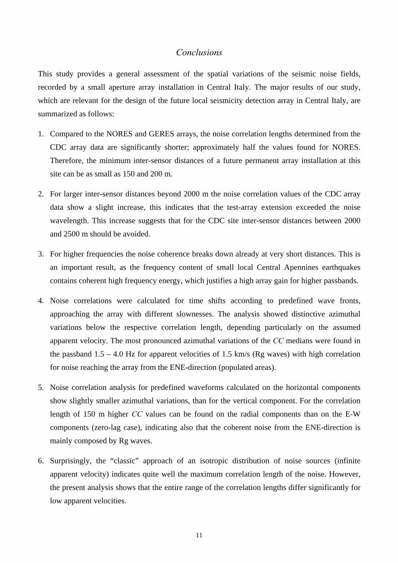
As test dataset, we use seismic data from a small aperture 9-element array, temporarily installed in
the Upper Tiber Valley, Italy near Città di Castello (CDC) during October 2000 (Braun et al., 2004). The instrumentation used during the experiment consisted of Lennartz 5800 digitizers (12 bit
gain ranged, sampling rate 125 sps) and LE 3D-5s seismometers. The installation of three
component sensors at all array sites allows the application of the array-analysis techniques to
horizontal-component data as well. Figure 1 shows the configuration of the CDC array with inter-
sensor distances varying between 150 and 2200 m.
Data acquisition of the array data was realized by a real-time acquisition system, based on a digital
data-transmission system (spread-spectrum). The technology of the mobile acquisition system
guaranteed a centralized timing, but it did neither allow continuous data acquisition nor the
possibility to change the preset sampling rate of 125 Hz (Braun et al., 2004). Therefore, as the CDC
array operated in an automatic amplitude-trigger mode, appropriate noise records necessary for the
present analysis had to be triggered manually. During the 13 days of operation, four noise samples
per day were recorded on average, with record lengths varying between 60 and 300 s. Although
noise samples are not available for all 24 hours, the dataset represents almost all relevant daytimes.
Special care had to be taken by excluding from the analysis all coherent 3 Hz “noise signals”, which
are known to be generated by industrial activities in the afternoon (see Figure 12 in Braun et al., 2004). These signals are characterized by monochromatic Rg-type ground movements with very
high coherence over the entire array (cross-correlation values > 0.9). The final selected set of noise
samples, observed over the whole array site, consists of 39 time windows with a total length of
8460 s.
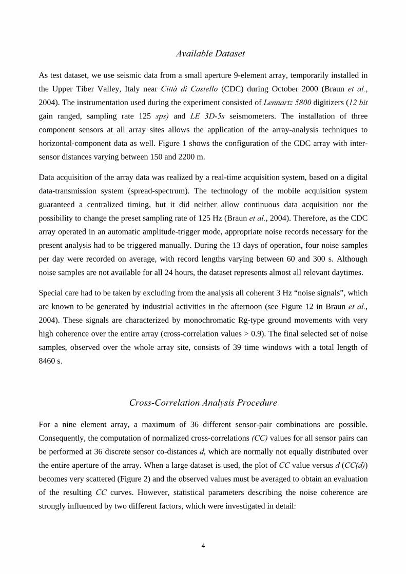
Cross-Correlation Analysis Procedure
For a nine element array, a maximum of 36 different sensor-pair combinations are possible.
Consequently, the computation of normalized cross-correlations (CC) values for all sensor pairs can
be performed at 36 discrete sensor co-distances d, which are normally not equally distributed over
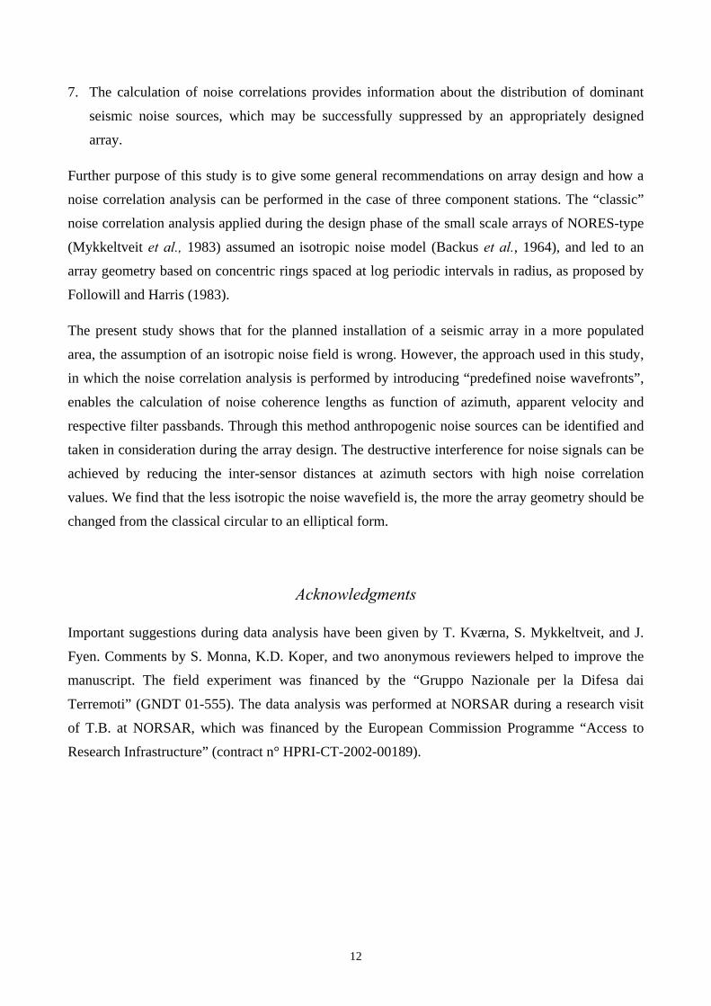
the entire aperture of the array. When a large dataset is used, the plot of CC value versus d (CC(d)) becomes very scattered (Figure 2) and the observed values must be averaged to obtain an evaluation
of the resulting CC curves. However, statistical parameters describing the noise coherence are
strongly influenced by two different factors, which were investigated in detail:
5
a) The time-window length of the noise sample, for a given distance, influences the spread of the
CC values around a mean value.
b) The choice of the binning intervals influences the actual CC value, calculated as representative
for a specific inter-sensor distance.
A first test concerned the influence of the length of the chosen noise window on the CC values. We
divided all noise records in contiguous and equally spaced time windows and calculated the
corresponding zero-lag CC values as function of the distance d between the sensors CC(d) for all
sensor-pair combinations. We performed four tests by choosing noise-window lengths of 5, 10, 20,
and 30 s, respectively. Since the statistical distribution of the CC values is non-Gaussian, average
CC values for each binning interval are defined by calculating the median and its ±1 quartile. While
on one hand the medians of the CC(d) values are nearly identical for the different windows, on the
other hand we observe a reduction of the respective interquartile ranges as the window length
increased. A window length of 20 s was found to be a reasonable choice for our analysis. In this
case, the influence of the extreme values on the median value defining CC(d) was less relevant, as it
resulted in narrower interquartile ranges.
The subdivision of the total 8460 s noise records into segments of 20 s leads to 423 time windows,
for which CC values are determined. CC calculations between all 36 inter-sensor combinations
provide 15,228 CC values as function of the respective inter-sensor distances. Figure 2 shows these
15,228 CC values as function of the Inter-sensor Distance (CID) for the 0.8 – 2.0 Hz frequency
band.
Since the observed CC values at one distance, or for a range of distances, are not equally
distributed, we show on all CID plots both the median and the +/-1 quartile range of the CC values.
The bin intervals for the inter-sensor distances were chosen to be 100 m long.
Amplitudes and shape of any seismic wave traversing an array will be more or less influenced by
scattering due to lateral heterogeneities and by attenuation of the seismic energy. Therefore, the
inter-sensor coherence of seismic signals is frequency dependent and all CC values have to be
investigated in different frequency bands. In this study, four filter bands were chosen to investigate
the noise behavior. Initially the noise coherence was investigated in seven filter bands, but it soon
turned out that for three high frequency filter bands (4 – 8 Hz, 5 – 10 Hz, and 6 – 12 Hz) the
observed correlation length at the CDC array was less than the minimum inter-sensor distance of
the array itself (130 m), i.e., the noise coherence in this frequency bands was practically zero. The
four remaining 3rd order Butterworth bandpass filters used in this study are listed in Table 1.
6
In the following sections, we compare the results of two different algorithms used to obtain the CC
values for data recorded with vertical components and filtered between 0.8 to 2.0 Hz:
• Zero-lag noise correlation (classic approach): without time shifts between the single traces, as in
the “classic” approach (e.g., Mykkeltveit et al., 1983; Mykkeltveit and Bungum, 1984; Kværna,
1989; Mykkeltveit et al., 1990; Harjes, 1990; Schweitzer et al., 2002).
• Noise correlation with predefined time lags for wavefront characteristics of the noise: applying
relative time shifts between the single traces that correspond to seismic signals approaching the
array with certain apparent velocities and backazimuth values (discretization of the slowness space).
The results for the three remaining filter bands of Table 1 and for the horizontal components are
presented and discussed after elucidating the two different algorithms.
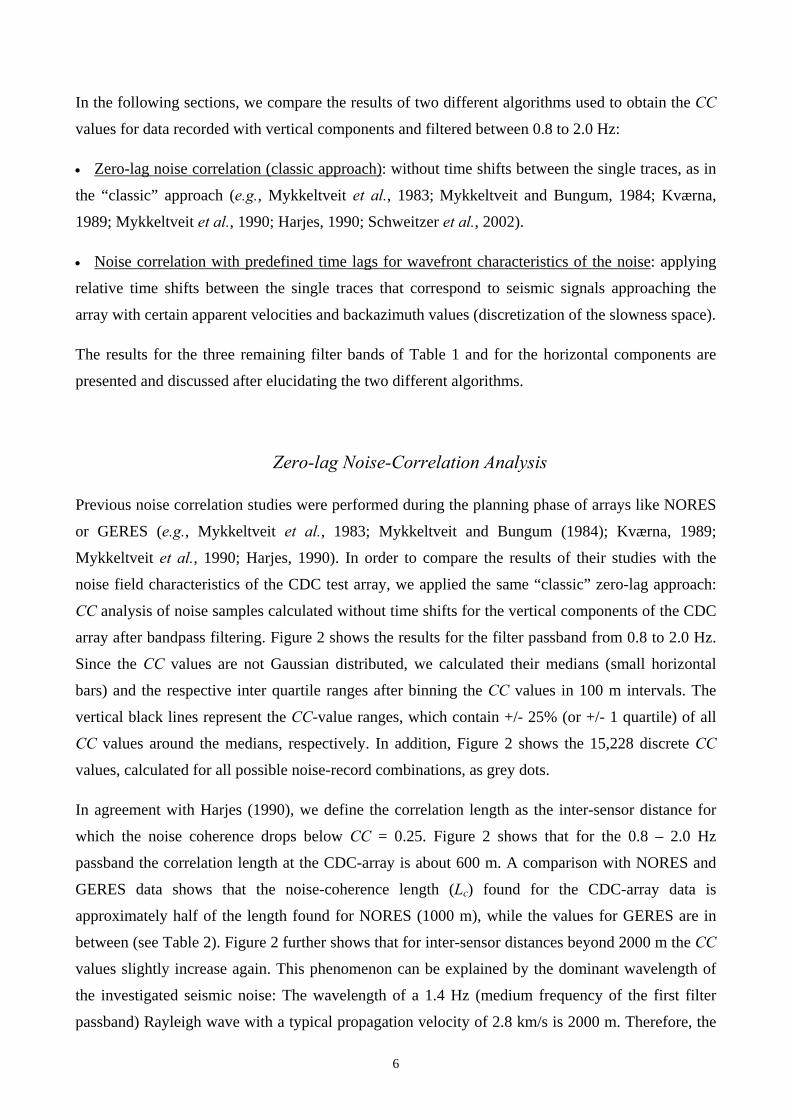
Zero-lag Noise-Correlation Analysis
Previous noise correlation studies were performed during the planning phase of arrays like NORES
or GERES (e.g., Mykkeltveit et al., 1983; Mykkeltveit and Bungum (1984); Kværna, 1989;
Mykkeltveit et al., 1990; Harjes, 1990). In order to compare the results of their studies with the
noise field characteristics of the CDC test array, we applied the same “classic” zero-lag approach:
CC analysis of noise samples calculated without time shifts for the vertical components of the CDC
array after bandpass filtering. Figure 2 shows the results for the filter passband from 0.8 to 2.0 Hz.
Since the CC values are not Gaussian distributed, we calculated their medians (small horizontal
bars) and the respective inter quartile ranges after binning the CC values in 100 m intervals. The
vertical black lines represent the CC-value ranges, which contain +/- 25% (or +/- 1 quartile) of all
CC values around the medians, respectively. In addition, Figure 2 shows the 15,228 discrete CC
values, calculated for all possible noise-record combinations, as grey dots.
In agreement with Harjes (1990), we define the correlation length as the inter-sensor distance for
which the noise coherence drops below CC = 0.25. Figure 2 shows that for the 0.8 – 2.0 Hz
passband the correlation length at the CDC-array is about 600 m. A comparison with NORES and
GERES data shows that the noise-coherence length (Lc) found for the CDC-array data is
approximately half of the length found for NORES (1000 m), while the values for GERES are in
between (see Table 2). Figure 2 further shows that for inter-sensor distances beyond 2000 m the CC
values slightly increase again. This phenomenon can be explained by the dominant wavelength of
the investigated seismic noise: The wavelength of a 1.4 Hz (medium frequency of the first filter
passband) Rayleigh wave with a typical propagation velocity of 2.8 km/s is 2000 m. Therefore, the
7
increase of the CC values can be explained by the similarity between two propagating noise waves,
only separated by one wavelength. Both, the smaller coherence length as well as the increase of the
CC values beyond 2000 m led to the conclusion that an array at the CDC location should have a
geometry with dominant inter-sensor distances between about 200 and 2000 m, at least when using
data between 0.8 and 2.0 Hz.
Mykkeltveit et al. (1983) found that the mean noise-correlation curves for NORES have a negative
minimum before tending to zero. In the case of azimuthal symmetry in the noise field or in inter-
sensor distances, the cross-spectral density C(ω,d) for propagating noise can be written as function
of the inter-sensor distance d:
dkkkdJkPdC ⋅⋅⋅= ∫∞
)(),(21),(
00ω
πω (1)
with P(ω,k) = frequency-wavenumber spectrum of the noise and J0(kd) = 0th order Bessel function
(see Mykkeltveit et al., 1983).
However, Harjes (1990) showed that noise-correlation curves at GERES smoothly decay without a
significant minimum. Starting from this observation he pointed out that the assumption of an
isotropic noise model – originally proposed by Backus et al., (1964) – might not be applicable to
arrays located in an azimuthally heterogeneous region. Also, the noise-correlation analysis of the
CDC data with the “classic” approach on the vertical components shows no significant negative
minimum and resembles the results of Harjes (1990). However, some CC values are negative and
may indicate that the original approach of azimuthal symmetry of the noise field by Mykkeltveit et al. (1983) may be applicable for some of our noise examples.
Noise-Correlation Analysis for Predefined Wavefront Characteristics
In the second approach, we search for coherent noise by evaluating the whole possible range of
positive and negative noise interference between the CDC sites. Since beamforming and other array
signal processing methods do not work with random time delays when using signals from different
array sites, we investigated possible dependencies of the noise correlation on wavefront propagation
characteristics, which are realistic for seismic signals. Therefore, we calculated relative time shifts
between the single traces, which corresponded to predefined (noise) wavefronts approaching the
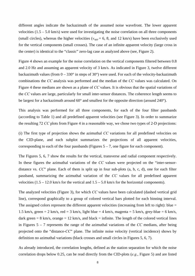
array under certain apparent velocities and backazimuth values. Figure 3 gives an overview of the
used wavefront parameters: The radius of the concentric circles represent the applied apparent
velocities, which span from typical values for regional P-type onsets to local Rg waves. The
8
different angles indicate the backazimuth of the assumed noise wavefront. The lower apparent
velocities (1.5 – 5.0 km/s) were used for investigating the noise correlation on all three components
(small circles), whereas the higher velocities (vapp = 6, 8, and 12 km/s) have been exclusively used
for the vertical components (small crosses). The case of an infinite apparent velocity (large cross in
the center) is identical to the “classic” zero-lag case as analyzed above (see, Figure 2).
Figure 4 shows an example for the noise correlation on the vertical components filtered between 0.8
and 2.0 Hz and assuming an apparent velocity of 3 km/s. As indicated in Figure 3, twelve different
backazimuth values (from 0 – 330° in steps of 30°) were used. For each of the velocity-backazimuth
combinations the CC analysis was performed and the median of the CC values was calculated. On
Figure 4 these medians are shown as a plane of CC values. It is obvious that the spatial variations of
the CC values are large, particularly for small inter-sensor distances. The coherence length seems to
be largest for a backazimuth around 60° and smallest for the opposite direction (around 240°).
This analysis was performed for all three components, for each of the four filter passbands
(according to Table 1) and all predefined apparent velocities (see Figure 3). In order to summarize
the resulting 72 CC plots from Figure 4 in a reasonable way, we chose two types of 2-D projections:
(i) The first type of projection shows the azimuthal CC variations for all predefined velocities on
the CID-plane, and each subplot summarizes the projections of all apparent velocities,
corresponding to each of the four passbands (Figures 5 – 7, one figure for each component).
The Figures 5, 6, 7 show the results for the vertical, transverse and radial component respectively.
In these figures the azimuthal variations of the CC values were projected on the “inter-sensor-
distance vs. CC” plane. Each of them is split up in four sub-plots (a, b, c, d), one for each filter
passband, summarizing the azimuthal variation of the CC values for all predefined apparent
velocities (1.5 – 12.0 km/s for the vertical and 1.5 – 5.0 km/s for the horizontal components).
The analyzed velocities (Figure 3), for which CC values have been calculated (dashed vertical grid
line), correspond graphically to a group of colored vertical bars plotted for each binning interval.
The assigned colors represent the different apparent velocities (increasing from left to right): blue =
1.5 km/s, green = 2 km/s, red = 3 km/s, light blue = 4 km/s, magenta = 5 km/s, grey-blue = 6 km/s,
dark green = 8 km/s, orange = 12 km/s, and black = infinite. The length of the colored vertical lines
in Figures 5 – 7 represents the range of the azimuthal variations of the CC medians, after being
projected onto the “distance-CC” plane. The infinite noise velocity (vertical incidence) shows by
definition no azimuthal variations (black crosses and small circles in Figures 5, 6, 7).
As already introduced, the correlation lengths, defined as the station separation for which the noise
correlation drops below 0.25, can be read directly from the CID-plots (e.g., Figure 5) and are listed
9
in Table 2 for the four different bandpass filters. Compared to NORES and GERES, the correlation
lengths determined from the CDC array data are shorter (approximately 50 – 60 % of the values
found for NORES). This observation suggests that an array installation in the Central Apennines
can reduce the inter-sensor distances without loosing its capability for reducing noise by destructive
interference.
Below the respective coherence lengths, distinct azimuthal variations of the noise correlation values
can be observed, especially for predefined wavefronts with low apparent velocities. The strongest
azimuthal variations among all three components can be found for vapp = 1.5 km/s, in the 2nd and 3rd
filter passband, between 1.5 – 4.0 Hz (e.g., at the binning interval around an inter-sensor distance of
150 m in Figure 5b). The azimuthal variations of the CC medians are smaller for the 3 – 4 Hz
passband, probably because the inter-sensor distance of 150 m is greater than the noise correlation
length. The azimuthal variations of the CC medians become smaller also as the apparent velocities
increases, converging towards a constant value for infinite velocity (zero-lag noise correlation).
At inter-sensor distances beyond the respective correlation length, the velocity-dependent variations
of the CC medians become less evident. In the 1.5 – 3 Hz passband of the vertical component
(Figure 5b), where the correlation length is about Lc = 300 m (Table 2), we observed that for inter-
sensor distances dis > Lc the variations of the CC medians become generally smaller. For other
values of inter-sensor distances (1150 m, 1250 m, 1750 m, 2250 m) the different color bars show
the same length, signifying that the (small) azimuthal variations of the CC medians do not depend
on the apparent velocity of the predefined noise wavefront.
The corresponding results for the transversal and radial components are shown in the Figures 6 and
7. Compared to Figure 5, the CC medians calculated for the transversal and the radial components
show slightly smaller variations. Figures 6 and 7 additionally show the CC medians for the zero-lag
noise correlations (infinite velocity). The zero-lag values are plotted with crosses (+) for the N-S
and with circles (o) for the E-W components. It is worth mentioning that in the bandpass filter 0.8 –
2 Hz (figures 6a, 7a) the CC medians for the inter-sensor distance dis = 150 m show higher values
on the E-W component, than on the N-S component, indicating that seismic noise reaching the array
from the ENE–direction (Figure 4), seems to be composed mainly by Rg-energy.
As shown in Figure 4, the correlation lengths are largest for the ENE-direction (60°) and shortest in
the opposite direction. Similar azimuthal characteristics are found for the CID-plots of the
remaining filter passbands of all three components (Figures 5, 6, 7). The reason for the strong
azimuthal variations of the correlation lengths may be caused by the distribution of the settlement
areas. The array was installed in a hilly zone in the western part of the sediment-filled Upper Tiber
Valley-plain. With respect to the array site, the urban areas (Città di Castello) are situated in the
10
ENE sector, whereas the western direction is characterized by an uninhabited hilly area, devoid of
potential men-made noise sources. The maximum correlation lengths observed in the ENE direction
(60°) may be caused by more monochromatic anthropogenic noise, generated in vicinity of the
small cities located inside the sediment-filled Tiber Valley.
(ii) The second type of projection summarizes in each subplot the azimuthal CC variations of the
correlation lengths as defined by a correlation coefficient of CC = 0.25 (see e.g., Harjes, 1990),
calculated for the four passbands from Table 1 (Figure 8). In this case the azimuthal variations of
the noise correlation lengths were read from CC curves as shown in Figure 4. This procedure allows
us to determine the azimuthal variations of the characteristic noise correlation length.
Figure 8 summarizes in each of the 18 subplots, the correlation length versus azimuth relation
calculated for the four passbands from Table 1. Different components can be distinguished by
different background colors: the first row (light grey) and the second row (white) show the results
for the radial and the transversal component, plotted for the S-velocity range from 1.5 to 5.0 km/s
and the two lower rows (dark grey) show results for the vertical component calculated for apparent
velocities between 1.5 and 12.0 km/s.
As already evidenced in Figure 4, distinct azimuthal variations of the noise correlation length can be
observed for all seismic components, filter bands and apparent velocities. The maximum/minimum
values are found at around 60° and 180° respectively, which were already explained to be caused by
nearby anthropogenic noise sources in the ENE sector. Also, the previously mentioned frequency-
and velocity dependence of the noise can be clearly observed in Figure 8 for all three components.
For the three higher passbands 1.5 – 3.0 Hz (x), 2.0 – 4.0 Hz (+), 3.0 – 6.0 Hz (*) the correlation
length decreases drastically with increasing apparent velocities. Whereas the amplitude of the
azimuthal variations of the correlation lengths for the passband 0.8 – 2.0 Hz (o) decreases, its mean
values remain stable at around 425 m, independently from the chosen apparent velocity.
Our study shows how an array should be designed for the Central Apennines in order to achieve
destructive interference for noise and account for azimuth dependent correlation lengths, by
arranging the sensors asymmetrically at reduced inter-sensor distances.
11
Conclusions
This study provides a general assessment of the spatial variations of the seismic noise fields,
recorded by a small aperture array installation in Central Italy. The major results of our study,
which are relevant for the design of the future local seismicity detection array in Central Italy, are
summarized as follows:
1. Compared to the NORES and GERES arrays, the noise correlation lengths determined from the
CDC array data are significantly shorter; approximately half the values found for NORES.
Therefore, the minimum inter-sensor distances of a future permanent array installation at this
site can be as small as 150 and 200 m.
2. For larger inter-sensor distances beyond 2000 m the noise correlation values of the CDC array
data show a slight increase, this indicates that the test-array extension exceeded the noise
wavelength. This increase suggests that for the CDC site inter-sensor distances between 2000
and 2500 m should be avoided.
3. For higher frequencies the noise coherence breaks down already at very short distances. This is
an important result, as the frequency content of small local Central Apennines earthquakes
contains coherent high frequency energy, which justifies a high array gain for higher passbands.
4. Noise correlations were calculated for time shifts according to predefined wave fronts,
approaching the array with different slownesses. The analysis showed distinctive azimuthal
variations below the respective correlation length, depending particularly on the assumed
apparent velocity. The most pronounced azimuthal variations of the CC medians were found in
the passband 1.5 – 4.0 Hz for apparent velocities of 1.5 km/s (Rg waves) with high correlation
for noise reaching the array from the ENE-direction (populated areas).
5. Noise correlation analysis for predefined waveforms calculated on the horizontal components
show slightly smaller azimuthal variations, than for the vertical component. For the correlation
length of 150 m higher CC values can be found on the radial components than on the E-W
components (zero-lag case), indicating also that the coherent noise from the ENE-direction is
mainly composed by Rg waves.
6. Surprisingly, the “classic” approach of an isotropic distribution of noise sources (infinite
apparent velocity) indicates quite well the maximum correlation length of the noise. However,
the present analysis shows that the entire range of the correlation lengths differ significantly for
low apparent velocities.
12
7. The calculation of noise correlations provides information about the distribution of dominant
seismic noise sources, which may be successfully suppressed by an appropriately designed
array.
Further purpose of this study is to give some general recommendations on array design and how a
noise correlation analysis can be performed in the case of three component stations. The “classic”
noise correlation analysis applied during the design phase of the small scale arrays of NORES-type
(Mykkeltveit et al., 1983) assumed an isotropic noise model (Backus et al., 1964), and led to an
array geometry based on concentric rings spaced at log periodic intervals in radius, as proposed by
Followill and Harris (1983).
The present study shows that for the planned installation of a seismic array in a more populated
area, the assumption of an isotropic noise field is wrong. However, the approach used in this study,
in which the noise correlation analysis is performed by introducing “predefined noise wavefronts”,
enables the calculation of noise coherence lengths as function of azimuth, apparent velocity and
respective filter passbands. Through this method anthropogenic noise sources can be identified and
taken in consideration during the array design. The destructive interference for noise signals can be
achieved by reducing the inter-sensor distances at azimuth sectors with high noise correlation
values. We find that the less isotropic the noise wavefield is, the more the array geometry should be
changed from the classical circular to an elliptical form.
Acknowledgments
Important suggestions during data analysis have been given by T. Kværna, S. Mykkeltveit, and J.
Fyen. Comments by S. Monna, K.D. Koper, and two anonymous reviewers helped to improve the
manuscript. The field experiment was financed by the “Gruppo Nazionale per la Difesa dai
Terremoti” (GNDT 01-555). The data analysis was performed at NORSAR during a research visit
of T.B. at NORSAR, which was financed by the European Commission Programme “Access to
Research Infrastructure” (contract n° HPRI-CT-2002-00189).
13
References
Backus, M. M., J. P. Burg, R. Baldwin, and E. Bryan (1964). Wide-band extraction of mantle P waves from ambient noise, Geophysics 29, 672-692.
Braun, T., J. Schweitzer, R. M. Azzara, D. Piccinini, M. Cocco, and E. Boschi (2004). Results from the temporary installation of a small aperture seismic array in the Central Apennines and its merits for the local event detection and location capabilities, Ann. Geophys. 47 (5), 1557-1568.
Followill F. and D. B. Harris (1983): Comments on Small aperture Array Design. Internal Report, Lawrence Livermore National Laboratory.
Fyen, J. (1990). Diurnal and seasonal variations in the microseismic noise level observed at the NORESS array, Phys. Earth Planet. Inter. 63, 252-268.
Harjes, H.-P. (1990). Design and siting of a new regional seismic array in Central Europe, Bull. Seism. Soc. Am. 80, 1801-1817.
Ingate S. F., E. S. Husebye, and A. Christofferson (1985). Regional Arrays and optimum data processing schemes, Bull. Seism. Soc. Am. 75, 1155-1177.
Kværna, T. (1989). On exploitation of small-aperture NORESS type arrays for enhanced P-wave detectability, Bull. Seism. Soc. Am. 79, 888-900.
Kværna, T. (1990). Sources of short-term fluctuations in the seismic noise level at NORESS, Phys. Earth Planet. Inter. 63, 269-276.
Mykkeltveit, S., K. Åstebøl, D. J. Dornboos, and E. S. Husebye (1983). Seismic array configuration optimization, Bull. Seism. Soc. Am. 73, 173-186.
Mykkeltveit, S., and H. Bungum (1984). Processing of regional seismic events using data from small-aperture arrays, Bull. Seism. Soc. Am. 74, 2313-2333.
Mykkeltveit, S. J. Fyen, F. Ringdal, and T. Kværna (1990). Spatial characteristics of the NORESS noise field and implications for array detection processing, Phys. Earth Planet. Int. 63, 277-283.
Piccinini, D., M. Cattaneo, C. Chiarabba, L. Chiaraluce, M. De Martin, M. Di Bona, M. Moretti, G. Selvaggi, P. Augliera, D. Spallarossa, G. Ferretti, A. Michelini, A. Govoni, P. Di Bartolomeo, M. Romanelli & J. Fabbri (2003): A microseismic study in a low seismicity area of Italy. The Città di Castello 2000 – 2001 experiment. Ann. Geophys., 46/6, 1315-1324.
Schweitzer, J., J. Fyen, S. Mykkeltveit, and T. Kværna (2002). Seismic Arrays, in IASPEI New Manual of Seismological Observatory Practice (NMSOP), P. Bormann (editor). GeoForschungsZentrum Potsdam, Vol. 1, Chapter 9, 52 pp.
14
Figure Captions
Figure 1. Location and configuration of the nine element test array, temporarily installed in the
Upper Tiber Valley near Città di Castello during October 2000. Each site (CA1 – CA9)
was equipped with a three component 5s-seismometer.
Figure 2. Normalized noise correlation values versus inter-sensor distances calculated for the
vertical components in the frequency band between 0.8 and 2.0 Hz as observed at the
CDC array.
Figure 3. Plot of the discrete slowness values simulating wavefronts of coherent noise. The radius
of the concentric rings represent the apparent velocities, and the angle the 12 different
backazimuth values (in steps of 30°). Small circles represent the velocities, for which this
study was performed for all three components (1.5 – 5.0 km/s); the velocities (12, 8, and
6 km/s) represented by small crosses have been exclusively used for noise-correlation
measurements on the vertical components.
Figure 4. Azimuthal variations of noise CC curves calculated for the vertical component of noise
records and assuming an apparent velocity of vapp = 3.0 km/s.
Figure 5. CC values (vertical component) for the data filtered with four different passbands (see
Table 1): (a) 0.8 – 2.0 Hz, (b) 1.5 – 3.0 Hz, (c) 2.0 – 4.0 Hz, (d) 3.0 – 6.0 Hz. At each
binning distance a group of colored vertical bars is plotted, representing the range of
medians found for all 12 azimuths at the 8 different beam velocities. Each group of bars
shows from left to right increasing apparent velocities, as defined in Figure 4. The crosses
show the infinite velocity results, which are not azimuth dependent.
Figure 6. Same as Figure 5 for the transverse component. The crosses and circles indicate the CC
medians found for the zero-lag noise correlations (infinite velocity) on the N-S
component (+) and the E-W component (o), respectively.
Figure 7. Same as Figure 6 for the radial component.
Figure 8. Correlation length at the CDC site as defined by a CC value of 0.25 plotted as function of
azimuth. Each of the 18 subplots shows the azimuthal variation of the correlation length
determined for the three components (R, T, Z) and the discrete apparent velocities shown
in Figure 3, calculated for the four passbands 0.8 – 2.0 Hz (o); 1.5 – 3.0 Hz (x); 2.0 – 4.0
Hz (+); and 3.0 – 6.0 Hz (*).
15
Table 1
Bandpass filters used for the presented CC analyses
Filter Frequency Passband
I 0.8 – 2.0 Hz
II 1.5 – 3.0 Hz
III 2.0 – 4.0 Hz
IV 3.0 – 6.0 Hz
Table 2
Noise-correlation lengths as measured for the vertical components of the CDC array (see Figures 2 and 5), the GERES array (Harjes, 1990), and the NORES array
(Mykkeltveit et al., 1983, Mykkeltveit et al., 1990)