Spatial variability of sensitive Champlain sea clay and anapplication of stochastic slope stability analysis of a cut
Paul Chiasson∗Faculté d’ingénierie, Université de Moncton, Moncton, NB, Canada
Yu-Jie WangDept of Geotechnical Eng., China Institute of Water Resources and Hydropower Research, Beijing, China
ABSTRACT: A stochastic slope stability analysis method is proposed to investigate short-term stabilityof unsupported excavation works in a soft clay deposit having spatially variable properties. Spatialvariability of undrained shear strength is modelled by a stochastic model that is the sum of a trendcomponent and a fluctuation component. The undrained shear strength trend, which is also spatiallyvariable, is modelled by a random function. Slope stability analyses are performed on the stochasticsoft clay model to investigate the contribution of spatial variability of undrained shear strength to adisagreement between high factors of safety computed from deterministic methods for slopes that havefailed. Probabilities of failure as computed from the stochastic analyses give a better assessment of failurepotential. Probability of failure values also correlate with time delay before failure. This phenomenonmay be related to progressive failure or creep and to pore-pressure dissipation with time.
1 INTRODUCTION
Short-term stability of unsupported excavation works is of great interest in geotechnical practice. Anaccurate evaluation of this type of stability is intimately dependent upon the applied analysis methodsand the representation of soil shear strength given as an input. Undrained shear strength as measured byfield vane testing is commonly used as an input for soil shear strength in total stress analyses. However,field undrained shear strengths, especially on sites involving soft, sensitive clay deposits, often presentstrong spatial variability (Soulié et al. 1990, Chiasson et al. 1995). In addition, estimates of undrainedshear strengths at locations where no measurements are available pose many questions. These two factorscannot be considered effectively in traditional deterministic total stress analyses, except, maybe, by theexperience of the designer.
Through detailed back analyses of a number of field embankments, Bjerrum (1972) found that directuse of undrained shear strength in total stress analyses overestimated the level of stability of embank-ments. Cases of cut slope failures were reported where a prior stability analysis gave factors of safetythat were greater than 1.0 (Bjerrum 1972, Lafleur et al. 1988). Many explanations for the disagree-ment between site observation and stability analysis have been postulated such as “time effect” and“anisotropy” (Bjerrum 1972) or “progressive failure” (Dascal & Tournier 1975). “Spatial variability”(Soulié et al. 1990, Chiasson et al. 1995) and uncertainty involved in estimation of undrained shearstrength could be other factors that are responsible for this disagreement.
As an attempt to model uncertainty and variability of soil shear strength, reliability analyses considershear strength as a random variable. A probability of failure or reliability index is obtained as a supplementto the deterministic factor of safety (Duncan 2000). Spatial variability of soil shear strength is, however,not considered in a reliability analysis, except by ad hoc approaches (El-Ramly et al. 2002). Using astochastic model for spatial variability of undrained shear strength (Chiasson et al. 1995), Chiasson &
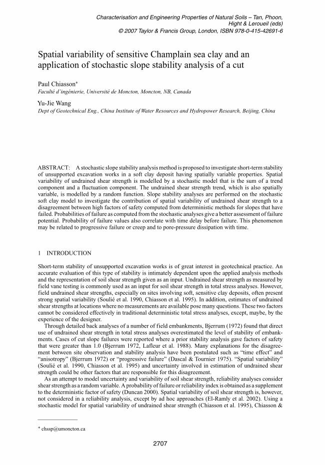
Figure 1. Site plan of St-Hilaire test excavation showing locations of vane profiles and slope failure scars (capitalletters A through F). Scale in metres.
Chiasson (2000) suggested a stochastic slope stability method to evaluate the failure risk rather than thedeterministic factor of safety. Undrained shear strength values were modeled as outcomes of a stochasticprocess.
Based on a well recorded test excavation work in spatially variable soft clay, this paper presents amodel for the spatial variability of undrained shear strength that combines a trend component with astochastic fluctuation (or residual) component. A random trend model for vane strength is also developed.The stochastic slope stability method is applied to investigate: (1) how spatial variability and uncertaintyof shear strength of a soil may be modeled and (2) how spatial variability of shear strength can explainthe disagreement between high deterministic factors of safety computed from a total stress analysis andthe fact that slope failures were observed at the site.
2 SUBSOIL AND SITE DESCRIPTION
To investigate short-term stability of unsupported cuts in soft sensitive clay deposits of eastern Canada,a test cut was excavated at a site near Sanit-Hilaire, approximately 50 kilometres to the east of Montréal,Canada (Lafleur et al. 1988). The crest of the excavation formed a 60 m by 60 m square in plan. It hadfour slopes: 18◦ (south slope), 27◦ (north slope), 34◦ (east slope), and 45◦ (west slope). Excavationdepth was of 6 m on the 45◦ west slope side and 8 m for the three other slopes (Figure 1). The site isunderlain by three distinctive soil layers (Figure 2). From the top, a thin 0.6 m layer of fine uniformbeach sand overlies a 2.0 to 3.0 m layer of weathered and fissured clay. Below, lies 30 m of sensitive andlightly overconsolidated Champlain Sea clay. A borehole 50 m to the north-east of the cut was haltedwhen a confined aquifer composed of a permeable glacial till (silty sand with some gravel) was reached.Installation of an open piezometer permitted to observe the presence of a small downward gradientthrough the clay and drained towards Richelieu River by the underlying confined aquifer.
An extensive subsoil exploration including vane tests (27 vane profiles as shown in Figure 1) wascarried out to determine the undrained shear strength of the clay deposit. Vane profiles extend up to 15.5 min depth with readings spaced each 0.50 m. Horizontal spacing between profiles is typically 10.0 m.
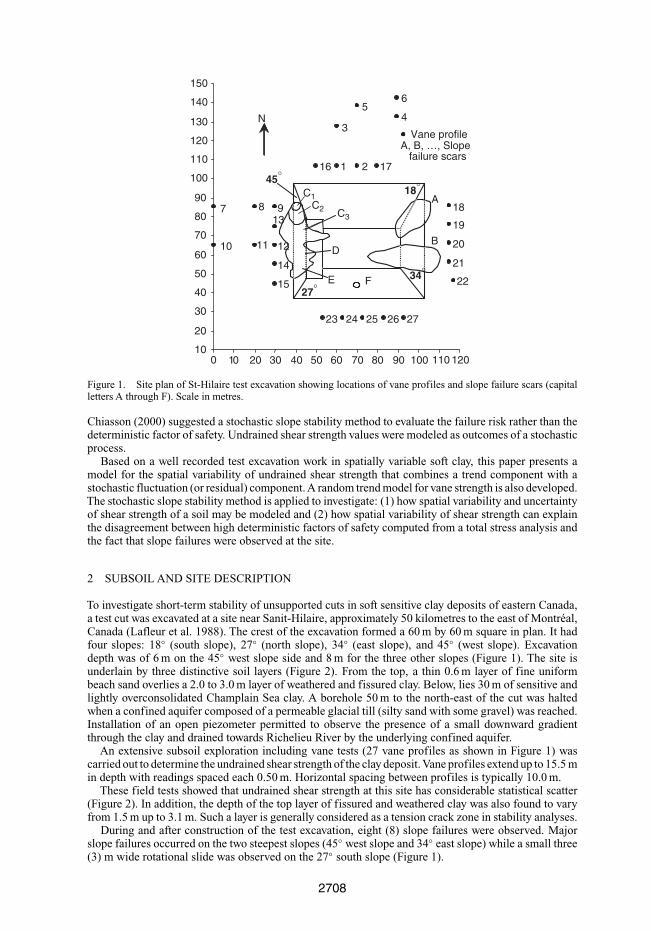
These field tests showed that undrained shear strength at this site has considerable statistical scatter(Figure 2). In addition, the depth of the top layer of fissured and weathered clay was also found to varyfrom 1.5 m up to 3.1 m. Such a layer is generally considered as a tension crack zone in stability analyses.
During and after construction of the test excavation, eight (8) slope failures were observed. Majorslope failures occurred on the two steepest slopes (45◦ west slope and 34◦ east slope) while a small three(3) m wide rotational slide was observed on the 27◦ south slope (Figure 1).
2708
40 80 120
Vane shear strength (kPa)
1 2 3
IL
0.00
4.00
8.00
12.00
16.00
0 50 100
Limits and water contents (%)D
epth
(m
)
wn
wP
wL
Figure 2. Typical geotechnical profile; wn, wP,wL and IL are respectively the natural water content, plasticity limit,liquidity limit and liquidity index.
3 MODELING SPATIAL VARIABILITY
Stationary processes can be modelled with the help of classical geostatistics. These processes have valuesthat fluctuate around a constant mathematical expectation. When considering a trend, a more generaltheory must be used. Matheron (1973) defined this theory as Intrinsic Random Functions of order k(IRF-k). Delfiner (1976) gives a more practical description, and his paper is recommended for thosereaders who wish more detailed explanations. Since the object of this paper is not to discuss this theoryin depth, a general description will be made using classical geostatistics as a working basis.
3.1 Stochastic modelling theory
In classical geostatistics, in situ parameters are considered as Regionalized Variables (RV) where region-alized indicates that the variable is intrinsically related to its spatial location. Since this variable cannotbe known everywhere, and it cannot be easily represented by a mathematical function, it is convenient toimagine the soil deposit as an outcome of a random process. This random process must take into accountthe regionalized character of the variable. Therefore not any type of random process is acceptable. Sta-tionary Random Functions (SRF) takes into account the regionalized character of a soil deposit. Let usthen represent an in situ parameter V (s) by the following:
where M (s) is the mathematical expectation at a given location vector s in space (a constant in a stationaryprocess), ε(s) is a zero mean stationary random function modelling fluctuations in function of locationvector s in space. When two outcomes ε(s) and ε(s + h) are close neighbours in space (small lag h), bothtake similar values, indicating high interdependency. When values (viewed as outcomes of the stochasticprocess) are far apart (large lag h), they tend to be independent of one another. Lag h where two valuesstart to be linearly independent is called the autocorrelation distance “a” or range of the spatial covarianceC(h). This covariance is defined as:
In a natural process, such as a soil deposit, this spatial covariance is a priori unknown. It has to beestimated. To do so, the preferred tool is the variogram 2γ (h), since by definition, it filters constants,and in stationary processes, the mean M of Equations 1 and 2 is a constant. Filtering the mathematicalexpectation implies that fluctuation variances are estimated without bias. The variogram is defined as:
2709
When the process is stationary, that is when M (s) is a constant mean whatever s, then the variogramsimplifies to:
When a finite variance exists, that is the stochastic process can be modelled as a SRF of order 2, thefollowing relation links the variogram to the spatial covariance C(h) at lag h:
where C(0) is the covariance at zero lag and corresponds to the variance of the SRF of order 2 of therandom function that is modelling the natural process fluctuations.
When a process is non stationary, the mean value M (s) (Equations 1 and 2) is no more a constant.This mean can be expressed, at least locally, by polynomials of degree k with unknown coefficients. Tocharacterize intrinsically V (s), that is to estimate C(h) of Equation (2), expressions of V (s) need to bemanipulated, and these expressions need to be independent of the polynomial coefficients.
In stationary processes, it was sufficient to use increments of order 0, [V (s + h) − V (s)], since theseincrements filter out the unknown constant mean. For polynomials of higher order k , increments oforder k need to be used to filter out the unknown polynomial trend. If this is an Intrinsic RandomFunction of order k (IRF-k), the variance of these increments exists and it can be expressed by acombination of generalized covariances (Matheron, 1973). In a stationary phenomenon IRF-k = 0, thesemi-variogram −γ (h) (half the variogram or semi-variogram) is a generalized covariance of order 0.
A regionalized variable can be modelled as the sum of a stationary random function of order 2 with adeterministic trend when the generalized covariance displays a sill (i.e. a horizontal threshold). In sucha case the relationship between the generalized covariance K(h) and the covariance C(h) is as followed:
where K(∞) represents the sill value of the generalized covariance. As a consequence, the relationshipbetween the generalized covariance and the variance C(0) is:
If K(0) = 0, then the variance is simply the amplitude of the generalized covariance sill.
3.2 A spatial variability model for vane strength, the fluctuation component
Vane strength shows a clear tendency to increase with depth (Figure 2). Computations of the followingmean first-order increment permits to evaluate how the variable should be modeled, that is as a stationaryor non stationary random function. The latter case implies a model for the trend, be it linear or of a higherorder.
where d(h) is the mean first-order increment for data spaced following a vertical axis by lag h and v(z)is the measured variable of interest at depth z. Measurements v(z) are in this case vane strengths cu.
By definition, the mean first-order increment filters constants. If random function V (z) is defined asV (z) = µ + ε(z), where µ is a constant mean and ε(z) is a random fluctuation with zero mean and setspatial covariance, then:
Thus, if the variable of interest fluctuates around a constant average value, that is it can be modeled as astationary random function, average increments will tend toward zero, regardless of lag h. On the otherhand, if the variable follows a trend, i.e. is it is non stationary, mean first-order increments will tend toincrease with lag h.
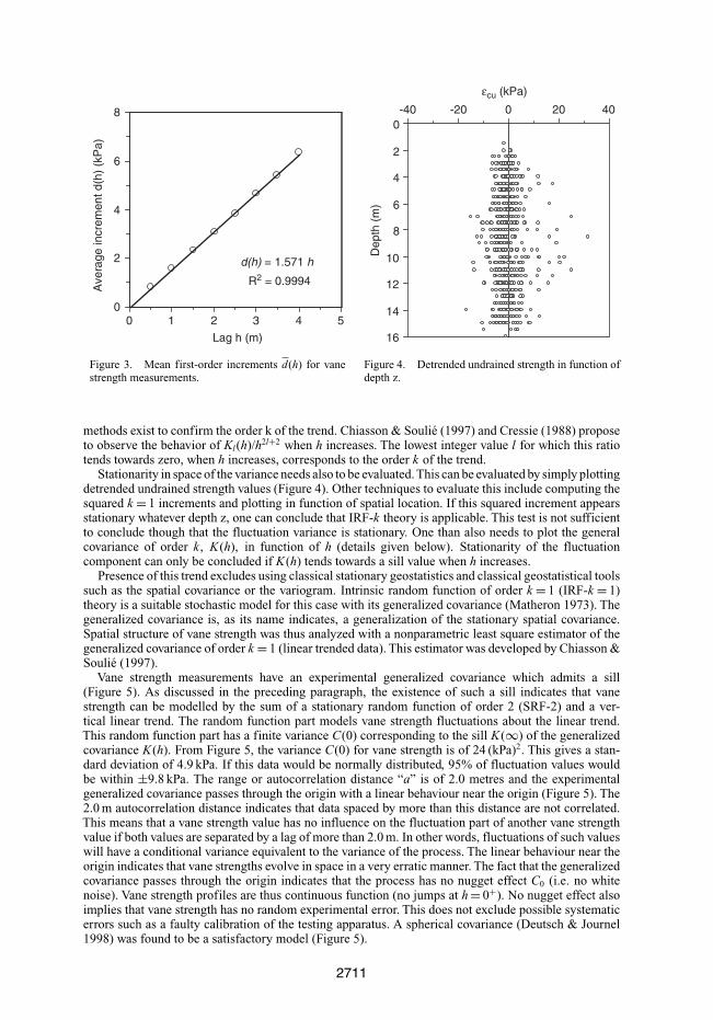
Mean-first order increments for vane strength and piezocone measurements are not zero at St-Hilaire.They increase linearly with lag h (Figure 3). Thus, vane strength values at St-Hilaire are not stationary.Similar results are found for piezocone data (Chiasson et al. 1995). The strong linearity of the first-orderincrements indicates that these measurements can be modeled as in Equation 1. Other more rigorous
2710
d(h) = 1.571 h
R2 = 0.9994
0
2
4
6
8
0 1 2 3 4 5
Lag h (m)
Ave
rage
incr
emen
t d(h
) (k
Pa)
Figure 3. Mean first-order increments d(h) for vanestrength measurements.
0
2
4
6
8
10
12
14
16
-40 -20 0 20 40
εcu (kPa)
Dep
th (
m)
Figure 4. Detrended undrained strength in function ofdepth z.
methods exist to confirm the order k of the trend. Chiasson & Soulié (1997) and Cressie (1988) proposeto observe the behavior of Kl(h)/h2l+2 when h increases. The lowest integer value l for which this ratiotends towards zero, when h increases, corresponds to the order k of the trend.
Stationarity in space of the variance needs also to be evaluated. This can be evaluated by simply plottingdetrended undrained strength values (Figure 4). Other techniques to evaluate this include computing thesquared k = 1 increments and plotting in function of spatial location. If this squared increment appearsstationary whatever depth z, one can conclude that IRF-k theory is applicable. This test is not sufficientto conclude though that the fluctuation variance is stationary. One than also needs to plot the generalcovariance of order k , K(h), in function of h (details given below). Stationarity of the fluctuationcomponent can only be concluded if K(h) tends towards a sill value when h increases.
Presence of this trend excludes using classical stationary geostatistics and classical geostatistical toolssuch as the spatial covariance or the variogram. Intrinsic random function of order k = 1 (IRF-k = 1)theory is a suitable stochastic model for this case with its generalized covariance (Matheron 1973). Thegeneralized covariance is, as its name indicates, a generalization of the stationary spatial covariance.Spatial structure of vane strength was thus analyzed with a nonparametric least square estimator of thegeneralized covariance of order k = 1 (linear trended data). This estimator was developed by Chiasson &Soulié (1997).
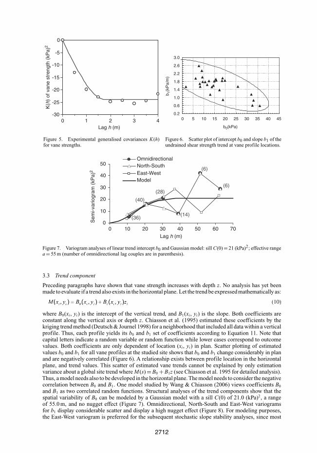
Vane strength measurements have an experimental generalized covariance which admits a sill(Figure 5). As discussed in the preceding paragraph, the existence of such a sill indicates that vanestrength can be modelled by the sum of a stationary random function of order 2 (SRF-2) and a ver-tical linear trend. The random function part models vane strength fluctuations about the linear trend.This random function part has a finite variance C(0) corresponding to the sill K(∞) of the generalizedcovariance K(h). From Figure 5, the variance C(0) for vane strength is of 24 (kPa)2. This gives a stan-dard deviation of 4.9 kPa. If this data would be normally distributed, 95% of fluctuation values wouldbe within ±9.8 kPa. The range or autocorrelation distance “a” is of 2.0 metres and the experimentalgeneralized covariance passes through the origin with a linear behaviour near the origin (Figure 5). The2.0 m autocorrelation distance indicates that data spaced by more than this distance are not correlated.This means that a vane strength value has no influence on the fluctuation part of another vane strengthvalue if both values are separated by a lag of more than 2.0 m. In other words, fluctuations of such valueswill have a conditional variance equivalent to the variance of the process. The linear behaviour near theorigin indicates that vane strengths evolve in space in a very erratic manner. The fact that the generalizedcovariance passes through the origin indicates that the process has no nugget effect C0 (i.e. no whitenoise). Vane strength profiles are thus continuous function (no jumps at h = 0+). No nugget effect alsoimplies that vane strength has no random experimental error. This does not exclude possible systematicerrors such as a faulty calibration of the testing apparatus. A spherical covariance (Deutsch & Journel1998) was found to be a satisfactory model (Figure 5).
Figure 6. Scatter plot of intercept b0 and slope b1 of theundrained shear strength trend at vane profile locations.
0
10
20
30
40
50
0 10 20 30 40 50 60 70Lag h (m)
Sem
i-var
iogr
am (
kPa)
2
OmnidirectionalNorth-SouthEast-WestModel
(36)
(40)
(28)
(14)
(6)
(6)
Figure 7. Variogram analyses of linear trend intercept b0 and Gaussian model: sill C(0) = 21 (kPa)2; effective rangea = 55 m (number of omnidirectional lag couples are in parenthesis).
3.3 Trend component
Preceding paragraphs have shown that vane strength increases with depth z. No analysis has yet beenmade to evaluate if a trend also exists in the horizontal plane. Let the trend be expressed mathematically as:
where B0(xi, yi) is the intercept of the vertical trend, and B1(xi, yi) is the slope. Both coefficients areconstant along the vertical axis or depth z. Chiasson et al. (1995) estimated these coefficients by thekriging trend method (Deutsch & Journel 1998) for a neighborhood that included all data within a verticalprofile. Thus, each profile yields its b0 and b1 set of coefficients according to Equation 11. Note thatcapital letters indicate a random variable or random function while lower cases correspond to outcomevalues. Both coefficients are only dependent of location (xi, yi) in plan. Scatter plotting of estimatedvalues b0 and b1 for all vane profiles at the studied site shows that b0 and b1 change considerably in planand are negatively correlated (Figure 6). A relationship exists between profile location in the horizontalplane, and trend values. This scatter of estimated vane trends cannot be explained by only estimationvariance about a global site trend where M (s) = B0 + B1z (see Chiasson et al. 1995 for detailed analysis).Thus, a model needs also to be developed in the horizontal plane. The model needs to consider the negativecorrelation between B0 and B1. One model studied by Wang & Chiasson (2006) views coefficients B0
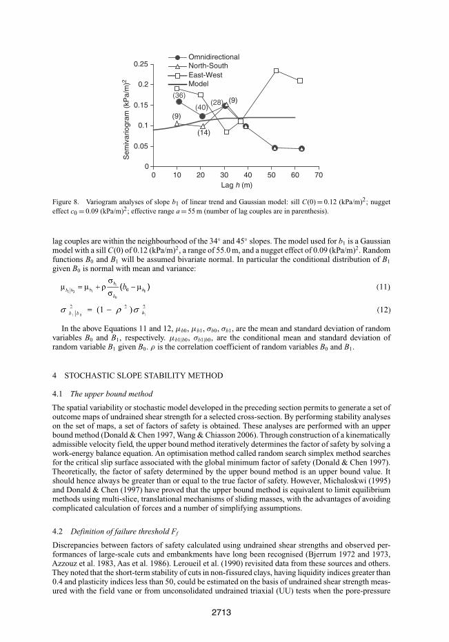
and B1 as two correlated random functions. Structural analyses of the trend components show that thespatial variability of B0 can be modeled by a Gaussian model with a sill C(0) of 21.0 (kPa)2, a rangeof 55.0 m, and no nugget effect (Figure 7). Omnidirectional, North-South and East-West variogramsfor b1 display considerable scatter and display a high nugget effect (Figure 8). For modeling purposes,the East-West variogram is preferred for the subsequent stochastic slope stability analyses, since most
2712
0
0.05
0.1
0.15
0.2
0.25
0 10 20 30 40 50 60 70Lag h (m)
Sem
ivar
iogr
am (
kPa/
m)2
OmnidirectionalNorth-SouthEast-WestModel
(36)
(9)
(14)
(9)(40)
(28)
Figure 8. Variogram analyses of slope b1 of linear trend and Gaussian model: sill C(0) = 0.12 (kPa/m)2; nuggeteffect c0 = 0.09 (kPa/m)2; effective range a = 55 m (number of lag couples are in parenthesis).
lag couples are within the neighbourhood of the 34◦ and 45◦ slopes. The model used for b1 is a Gaussianmodel with a sill C(0) of 0.12 (kPa/m)2, a range of 55.0 m, and a nugget effect of 0.09 (kPa/m)2. Randomfunctions B0 and B1 will be assumed bivariate normal. In particular the conditional distribution of B1
given B0 is normal with mean and variance:
In the above Equations 11 and 12, µb0, µb1, σb0, σb1, are the mean and standard deviation of randomvariables B0 and B1, respectively. µb1|b0, σb1|b0, are the conditional mean and standard deviation ofrandom variable B1 given B0. ρ is the correlation coefficient of random variables B0 and B1.
4 STOCHASTIC SLOPE STABILITY METHOD
4.1 The upper bound method
The spatial variability or stochastic model developed in the preceding section permits to generate a set ofoutcome maps of undrained shear strength for a selected cross-section. By performing stability analyseson the set of maps, a set of factors of safety is obtained. These analyses are performed with an upperbound method (Donald & Chen 1997, Wang & Chiasson 2006). Through construction of a kinematicallyadmissible velocity field, the upper bound method iteratively determines the factor of safety by solving awork-energy balance equation. An optimisation method called random search simplex method searchesfor the critical slip surface associated with the global minimum factor of safety (Donald & Chen 1997).Theoretically, the factor of safety determined by the upper bound method is an upper bound value. Itshould hence always be greater than or equal to the true factor of safety. However, Michaloskwi (1995)and Donald & Chen (1997) have proved that the upper bound method is equivalent to limit equilibriummethods using multi-slice, translational mechanisms of sliding masses, with the advantages of avoidingcomplicated calculation of forces and a number of simplifying assumptions.
4.2 Definition of failure threshold Ff
Discrepancies between factors of safety calculated using undrained shear strengths and observed per-formances of large-scale cuts and embankments have long been recognised (Bjerrum 1972 and 1973,Azzouz et al. 1983, Aas et al. 1986). Leroueil et al. (1990) revisited data from these sources and others.They noted that the short-term stability of cuts in non-fissured clays, having liquidity indices greater than0.4 and plasticity indices less than 50, could be estimated on the basis of undrained shear strength meas-ured with the field vane or from unconsolidated undrained triaxial (UU) tests when the pore-pressure
Figure 9. Factors of safety obtained by total stress analyses of short-term failures (Ff ST ) versus the plasticity index.Case where IL > 0.4 and IP < 50 (adapted from Leroueil et al. 1990).
redistribution is not significant. A least square line obtained from their data is plotted at Figure 9. Itsequation is:
This line is close to the trend first proposed by Bjerrum (1972, 1973). At St-Hilaire, the averageplasticity index for a depth range of 2.5 to 8.0 m is 29.7 ± 1.8%. Thus, based on the above equation,slopes that have a computed, short term, total stress factor of safety of 1.087 will on average fail atSt-Hilaire (Figure 9). In this paper, this value is defined as the factor of safety at failure threshold (Ff ).If the computed factor of safety Fos is equal or less than Ff , the slope is in a state of failure.
4.3 Definition of probability of failure
For N cross-sectional outcome maps of undrained shear strength, there are accordingly N factors ofsafety that are obtained. If there are M factors of safety less than the failure threshold Ff , a “CalculatedProbability of Failure” is defined as Pfc = M/N. If there are no factors of safety less than the failurethreshold Ff , or not enough for a reliable statistical prediction within the N outcomes, a statisticaldistribution of the factor of safety needs to be estimated first. A “Nominal Probability of Failure” Pfn
is then defined as the probability of the event of Fos ≤ Ff based on the approximate distribution. Forexample, if the factor of safety is assumed to be normally distributed, the nominal probability of failurewould be determined by:
In this paper, all values of probability of failure are of the calculated type.
4.4 Results from stochastic analyses
As shown in Figure 1, eight (8) slides occurred along 45◦, 34◦, and 27◦ slopes during and after excavation.In order to explore the excavation behaviour in terms of cut depth, 2-D stochastic slope stability analysesare performed for a number of cross-sections passing through vane profiles Su9, Su13, Su12, Su14 andSu15 for the 45◦ slope, Su19, Su20, Su21 for the 34◦ slope, and Su25 for the 27◦ slope. These cross-sections are relatively well centred with observed failure scars. Water contents for the top fissured clayand the underlying intact clay deposit are assumed to be 40% and 50% respectively. These are averagesite values. Water content for the studied site ranges between 34% and 99%, with a standard deviation of7%. Average water contents of 40% (top fissured clay) and 50% (intact clay) correspond to unit weights
2714
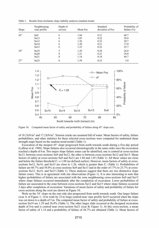
Table 1. Results from stochastic slope stability analyses (random trend).
Neighbouring Depth of Standard Probability ofSlope vane profile cut (m) Mean Fos deviation of Fos failure (%)
Figure 10. Computed mean factor of safety and probability of failure along 45◦ slope axis.
of 18.2 kN/m3 and 17.2 kN/m3. Tension cracks are assumed full of water. Mean factors of safety, failureprobabilities, and other statistics for these selected cross-sections were computed for undrained shearstrength maps based on the random trend model (Table 1).
Excavation of the steepest 45◦ slope progressed from north towards south during a five-day period(Lafleur et al. 1988). Slope failures also occurred chronologically in the same order once the excavationreached a depth of 6 m. Two major slope failure zones can be identified; one is centred at cross-sectionSu13, between cross-sections Su9 and Su12, the other is between cross-sections Su12 and Su15. Meanfactors of safety at cross-sections Su9 and Su13 are 1.04 and 1.05 (Table 1). All these values are closeand below the failure threshold Ff = 1.09 (as defined earlier). However, mean factors of safety at cross-sections Su12, Su14, and Su15 are close to 1.26, which is greater than Ff (Table 1). Probabilities offailure are 60.7% and 58.0% at cross-sections Su9 and Su13 and in the order of 17% to 25.7% at cross-sections Su12, Su14, and Su15 (Table 1). These analyses suggest that there are two distinctive slopefailure zones. This is in agreement with site observations (Figure 1). It is also interesting to note thathigher probabilities of failure are associated with the zone neighbouring cross-sections Su9 and Su13where slope failures occurred immediately after the completion of excavation. Lower probabilities offailure are associated to the zone between cross-sections Su12 and Su15 where slope failures occurred3 days after completion of excavation. Variations of mean factor of safety and probability of failure forcross-sections along the crest are shown in Figure 10.
Work on the 34◦ slope on the east side also progressed from north towards south. One larger failure(scar A of Figure 1; 14 m wide by 23 m long) centred near vane profile Su19 occurred when the slopewas cut down to a depth of 5 m. The computed mean factor of safety and probability of failure at cross-section Su19 are 1.29 and 26.0% (Table 1). The other larger slide occurred at the designed excavationdepth of 8 m and is centred near cross-section Su21 (scar B, Figure 1). At this cross-section, a meanfactor of safety of 1.14 and a probability of failure of 44.7% are obtained (Table 1). Mean factors of
2715
0.4
0.5
0.6
0.7
0.8
0.9
1
1.1
1.2
1.3
1.4
40 50 60 70 80 90
South towards north transect (m)
Mea
n F
os
0%
20%
40%
60%
80%
100%
Pro
babi
lity
of fa
ilure
Mean Fos
pf
Su21 Su20 Su19
Ff = 1.09
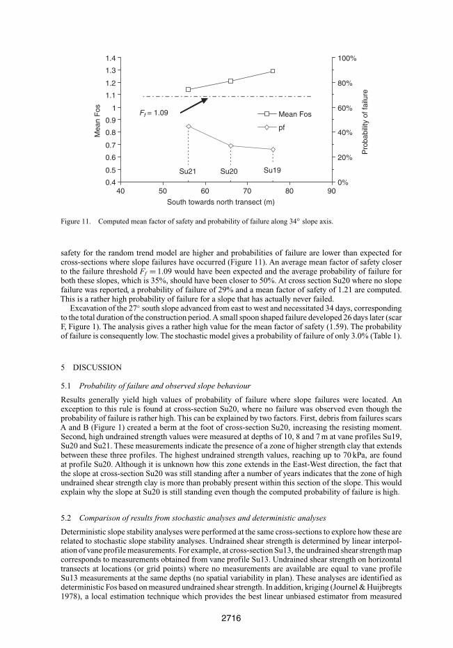
Figure 11. Computed mean factor of safety and probability of failure along 34◦ slope axis.
safety for the random trend model are higher and probabilities of failure are lower than expected forcross-sections where slope failures have occurred (Figure 11). An average mean factor of safety closerto the failure threshold Ff = 1.09 would have been expected and the average probability of failure forboth these slopes, which is 35%, should have been closer to 50%. At cross section Su20 where no slopefailure was reported, a probability of failure of 29% and a mean factor of safety of 1.21 are computed.This is a rather high probability of failure for a slope that has actually never failed.
Excavation of the 27◦ south slope advanced from east to west and necessitated 34 days, correspondingto the total duration of the construction period. A small spoon shaped failure developed 26 days later (scarF, Figure 1). The analysis gives a rather high value for the mean factor of safety (1.59). The probabilityof failure is consequently low. The stochastic model gives a probability of failure of only 3.0% (Table 1).
5 DISCUSSION
5.1 Probability of failure and observed slope behaviour
Results generally yield high values of probability of failure where slope failures were located. Anexception to this rule is found at cross-section Su20, where no failure was observed even though theprobability of failure is rather high. This can be explained by two factors. First, debris from failures scarsA and B (Figure 1) created a berm at the foot of cross-section Su20, increasing the resisting moment.Second, high undrained strength values were measured at depths of 10, 8 and 7 m at vane profiles Su19,Su20 and Su21. These measurements indicate the presence of a zone of higher strength clay that extendsbetween these three profiles. The highest undrained strength values, reaching up to 70 kPa, are foundat profile Su20. Although it is unknown how this zone extends in the East-West direction, the fact thatthe slope at cross-section Su20 was still standing after a number of years indicates that the zone of highundrained shear strength clay is more than probably present within this section of the slope. This wouldexplain why the slope at Su20 is still standing even though the computed probability of failure is high.
5.2 Comparison of results from stochastic analyses and deterministic analyses
Deterministic slope stability analyses were performed at the same cross-sections to explore how these arerelated to stochastic slope stability analyses. Undrained shear strength is determined by linear interpol-ation of vane profile measurements. For example, at cross-section Su13, the undrained shear strength mapcorresponds to measurements obtained from vane profile Su13. Undrained shear strength on horizontaltransects at locations (or grid points) where no measurements are available are equal to vane profileSu13 measurements at the same depths (no spatial variability in plan). These analyses are identified asdeterministic Fos based on measured undrained shear strength. In addition, kriging (Journel & Huijbregts1978), a local estimation technique which provides the best linear unbiased estimator from measured
2716
Table 2. Comparison of factors of safety between stochastic and deterministic methods.
Deterministic FosNeighbouring Stochastic
Slope vane profile Depth (m) mean Fos Measured Cu Kriged Cu
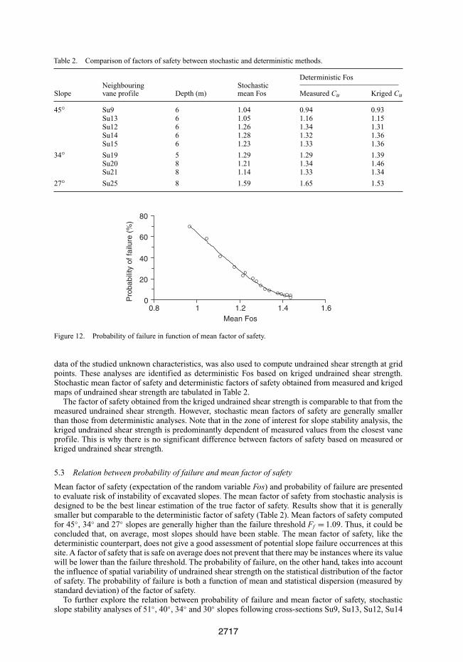
Figure 12. Probability of failure in function of mean factor of safety.
data of the studied unknown characteristics, was also used to compute undrained shear strength at gridpoints. These analyses are identified as deterministic Fos based on kriged undrained shear strength.Stochastic mean factor of safety and deterministic factors of safety obtained from measured and krigedmaps of undrained shear strength are tabulated in Table 2.
The factor of safety obtained from the kriged undrained shear strength is comparable to that from themeasured undrained shear strength. However, stochastic mean factors of safety are generally smallerthan those from deterministic analyses. Note that in the zone of interest for slope stability analysis, thekriged undrained shear strength is predominantly dependent of measured values from the closest vaneprofile. This is why there is no significant difference between factors of safety based on measured orkriged undrained shear strength.
5.3 Relation between probability of failure and mean factor of safety
Mean factor of safety (expectation of the random variable Fos) and probability of failure are presentedto evaluate risk of instability of excavated slopes. The mean factor of safety from stochastic analysis isdesigned to be the best linear estimation of the true factor of safety. Results show that it is generallysmaller but comparable to the deterministic factor of safety (Table 2). Mean factors of safety computedfor 45◦, 34◦ and 27◦ slopes are generally higher than the failure threshold Ff = 1.09. Thus, it could beconcluded that, on average, most slopes should have been stable. The mean factor of safety, like thedeterministic counterpart, does not give a good assessment of potential slope failure occurrences at thissite. A factor of safety that is safe on average does not prevent that there may be instances where its valuewill be lower than the failure threshold. The probability of failure, on the other hand, takes into accountthe influence of spatial variability of undrained shear strength on the statistical distribution of the factorof safety. The probability of failure is both a function of mean and statistical dispersion (measured bystandard deviation) of the factor of safety.
To further explore the relation between probability of failure and mean factor of safety, stochasticslope stability analyses of 51◦, 40◦, 34◦ and 30◦ slopes following cross-sections Su9, Su13, Su12, Su14
2717
0.2 0.4 0.6 0.8 1.0 1.2 1.4 1.6 1.8
Fos
-4
-3
-2
-1
0
1
2
3
4
Exp
ecte
d N
orm
al V
alue
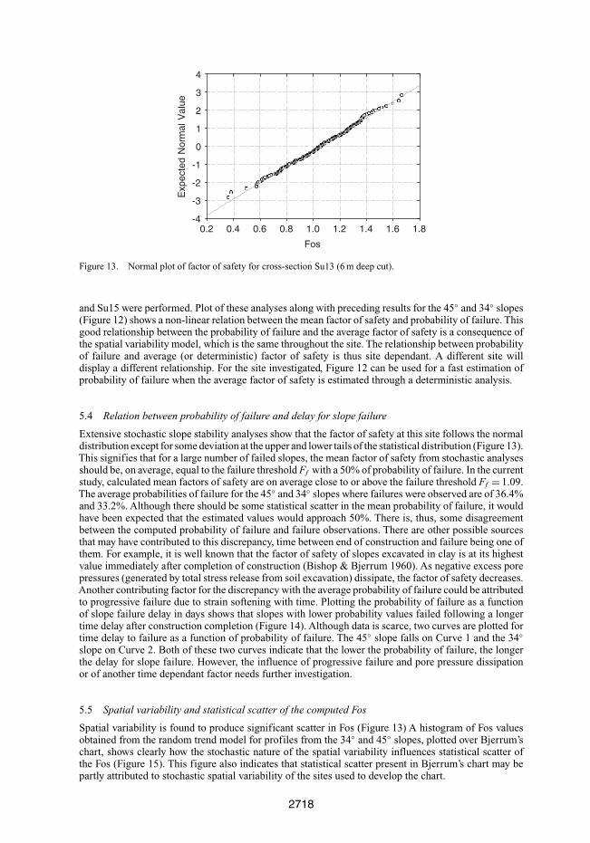
Figure 13. Normal plot of factor of safety for cross-section Su13 (6 m deep cut).
and Su15 were performed. Plot of these analyses along with preceding results for the 45◦ and 34◦ slopes(Figure 12) shows a non-linear relation between the mean factor of safety and probability of failure. Thisgood relationship between the probability of failure and the average factor of safety is a consequence ofthe spatial variability model, which is the same throughout the site. The relationship between probabilityof failure and average (or deterministic) factor of safety is thus site dependant. A different site willdisplay a different relationship. For the site investigated, Figure 12 can be used for a fast estimation ofprobability of failure when the average factor of safety is estimated through a deterministic analysis.
5.4 Relation between probability of failure and delay for slope failure
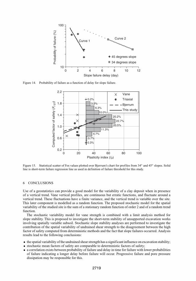
Extensive stochastic slope stability analyses show that the factor of safety at this site follows the normaldistribution except for some deviation at the upper and lower tails of the statistical distribution (Figure 13).This signifies that for a large number of failed slopes, the mean factor of safety from stochastic analysesshould be, on average, equal to the failure threshold Ff with a 50% of probability of failure. In the currentstudy, calculated mean factors of safety are on average close to or above the failure threshold Ff = 1.09.The average probabilities of failure for the 45◦ and 34◦ slopes where failures were observed are of 36.4%and 33.2%. Although there should be some statistical scatter in the mean probability of failure, it wouldhave been expected that the estimated values would approach 50%. There is, thus, some disagreementbetween the computed probability of failure and failure observations. There are other possible sourcesthat may have contributed to this discrepancy, time between end of construction and failure being one ofthem. For example, it is well known that the factor of safety of slopes excavated in clay is at its highestvalue immediately after completion of construction (Bishop & Bjerrum 1960). As negative excess porepressures (generated by total stress release from soil excavation) dissipate, the factor of safety decreases.Another contributing factor for the discrepancy with the average probability of failure could be attributedto progressive failure due to strain softening with time. Plotting the probability of failure as a functionof slope failure delay in days shows that slopes with lower probability values failed following a longertime delay after construction completion (Figure 14). Although data is scarce, two curves are plotted fortime delay to failure as a function of probability of failure. The 45◦ slope falls on Curve 1 and the 34◦slope on Curve 2. Both of these two curves indicate that the lower the probability of failure, the longerthe delay for slope failure. However, the influence of progressive failure and pore pressure dissipationor of another time dependant factor needs further investigation.
5.5 Spatial variability and statistical scatter of the computed Fos
Spatial variability is found to produce significant scatter in Fos (Figure 13) A histogram of Fos valuesobtained from the random trend model for profiles from the 34◦ and 45◦ slopes, plotted over Bjerrum’schart, shows clearly how the stochastic nature of the spatial variability influences statistical scatter ofthe Fos (Figure 15). This figure also indicates that statistical scatter present in Bjerrum’s chart may bepartly attributed to stochastic spatial variability of the sites used to develop the chart.
2718
10
100
0 2 4 6 8 10 12
Slope failure delay (day)
Pro
babi
lity
of fa
ilure
(%
)45 degrees slope
34 degrees slope
Curve 1Curve 2
Figure 14. Probability of failure as a function of delay for slope failure.
0.3%
0.7%
4.7%
11.3%
20.5%
22.7%
20.2%
10.0%
6.3%
3.2%
0.2%
0.20 20 40 60 80 100
0.6
1.0
1.4
1.8
2.2
Plasticity index (IP)
Com
pute
d fa
ctor
of s
afet
y (F
f ST)
Vane
Triaxial
Bjerrum
This study
Figure 15. Statistical scatter of Fos values plotted over Bjerrum’s chart for profiles from 34◦ and 45◦ slopes. Solidline is short-term failure regression line as used in definition of failure threshold for this study.
6 CONCLUSIONS
Use of a geostatistics can provide a good model for the variability of a clay deposit when in presenceof a vertical trend. Vane vertical profiles, are continuous but erratic functions, and fluctuate around avertical trend. These fluctuations have a finite variance, and the vertical trend is variable over the site.This later component is modelled as a random function. The proposed stochastic model for the spatialvariability of the studied site is the sum of a stationary random function of order 2 and of a random trendfunction.
The stochastic variability model for vane strength is combined with a limit analysis method forslope stability. This is proposed to investigate the short-term stability of unsupported excavation worksinvolving spatially variable subsoil. Stochastic slope stability analyses are performed to investigate thecontribution of the spatial variability of undrained shear strength to the disagreement between the highfactor of safety computed from deterministic methods and the fact that slope failures occurred. Analysisresults lead to the following conclusions:
• the spatial variability of the undrained shear strength has a significant influence on excavation stability;• stochastic mean factors of safety are comparable to deterministic factors of safety;• a correlation exists between probability of failure and delay in time for failure with lower probabilities
of failure indicating a longer delay before failure will occur. Progressive failure and pore pressuredissipation may be responsible for this.
2719
ACKNOWLEDGEMENTS
Funding for this research work was provided by grant OGP013720 of the National Science and Engin-eering Research Council of Canada (NSERC) and by the China National Natural Science Foundation,grant No. 50539100 and No. 50509027. The authors are also grateful to the Université de Monctonfor its financial and technical support and to the China Institute of Water Resources and HydropowerResearch (IWHR).
REFERENCES
Aas, Gunnar, Lacasse, Suzanne, Lunne, Tom, & Hoeg, Kaare. 1986. Use of in situ tests for foundation designon clay. In Samuel P Clemence (ed.), Use of in situ tests in geotechnical engineering : Proc. of In Situ ’86, aspecialty conference,VirginiaTech, Blacksburg,Virginia, 23–25 June 1986, Geotechnical Special Publ No. 6: 1–30.New York: ASCE.
Azzouz, Amr S., Baligh, Mohsen M. & Ladd, Charles C. 1983. Corrected field vane strength for embankment design.Journal of Geotechnical Engineering 109(5): 730–734.
Bishop, A.W. & Bjerrum, L. 1960. The relevance of the triaxial test to the solution of stability problems. In ResearchConference on Shear Strength of Cohesive soils. Boulder, Co.: 437–501. New York: ASCE.
Bjerrum, L. 1972. Embankments on soft ground. In Performance of Earth Supported Structures, Proceedings of theSpeciality Conference, Lafayette, IN, 11–14 June 1972: 2: 1–54. New York: ASCE.
Bjerrum, L. 1973. Problems of soil mechanics and construction on soft clays, State-of-the-Art report to Session 4. In8th International Conference on Soil Mechanics and Foundation Engineering, Proc., Moscow: 3: 111–159.
Chiasson, B. & Chiasson P. 2000. Slope stability by limit analysis and stochastic conditioning. In Proceedings ofGeoEng 2000: An International Conference on Geotechnical & Geological Engineering, Melbourne, Australia,19–24 November 2000, CD-ROM, 5p. Lancaster, PA, USA: Technomic Publishing Co.
Chiasson, P., Lafleur, J., Soulié, M. & Law, K.T. 1995. Characterizing spatial variability of a clay by geostatistics.Canadian Geotechnical Journal 32(1): 1–10.
Chiasson, P. & Souié, M. 1997. Nonparametric estimation of generalized covariances by modeling on-line data.Mathematical Geology 29(1): 153–172.
Cressie, N.A. 1988. A graphical procedure for determining nonstationarity in time series. Jour. Am. Stat. Assoc.19(5):425–449.
Dascal, O. & Tournier, J.-P. 1975. Embankments on soft and sensitive clay foundation. Journal of the GeotechnicalEngineering Division, ASCE 101(3): 297–314.
Delfiner, P. 1976. Linear Estimation of Non Stationary Spatial Phenomena. In Advanced Geostatistics in the MiningIndustry, Proc. of NATO-ASI, Rome: 49–68. Dordrecht, Netherlands: D. Reidel Pub.
Deutsch, C.V. & Journel, A.G. 1998. GSLIB: Geostatistical software library and user’s guide. New York: OxfordUniversity Press.
Djebbari, Z. 1996. Simulation géostatistique et calcul de stabilité de pente par programmation dynamique, M.Sc.A.Thesis, Moncton, NB, Canada : Université de Moncton, Faculté d’ingénierie.
Donald, I.B. & Chen, Z. 1997. Slope stability analysis by the upper bound approach: fundamentals and methods.Canadian Geotechnical Journal 34(6): 853–862.
Duncan, J.M. 2000. Factors of safety and reliability in geotechnical engineering. Journal of Geotechnical andGeoenvironmental Engineering, ASCE 126(4): 307–316.
El-Ramly, H., Morgenstern, N.R. & Cruden, D.M. 2003. Probabilistic slope stability analysis of a tailings dyke onpresheared clay-shale. Canadian Geotechnical Journal 40(1): 192–208.
Journel, A.G. & Huijbregts, C.J. 1978. Mining geostatistics. London: Academic press.Lafleur, J., Silvestri, V., Asselin, R. & Soulié, M. 1988. Behaviour of a test excavation in soft Champlain Sea clay.
Canadian Geotechnical Journal 25(4): 705–715.Leroueil, S., La Rochelle, P., Tavenas, F. & Roy, M. 1990. Remarks on the stability of temporary cuts. Canadian
Geotechnical Journal 27(5): 687–692.Lunne, T., Robertson, P.K. & Powell J.J.M. 1997. Cone Penetration testing in geotechnical practice. New York:
Blackie Academic & Professional.Matheron, G. 1973. The Intrinsic Random Functions and their Applications. Advances in Applied Probability, 5:
439–469.Michalowski, R.L. 1995. Slope stability analysis: a kinematical approach. Geotéchnique 45: 283–293.Soulié, M., Montès, P. & Silverstri, V. 1990. Modelling spatial variability of soil parameters. Canadian Geotechnical
Journal 27(5): 617–630.Wang, Y.-J. 2001. Stability Analysis of Slopes and Footings Considering Different Dilation Angles of Geomaterial.
Ph.D. thesis, Hong Kong: Department of Civil and Structural Engineering, Hong Kong Polytechnic University.Wang, Y.-J. & Chiasson, P. 2006 (Accepted). Stochastic Stability Analysis of a Test Excavation Involving Spatially