On the local odds ratio between points andmarks in marked point processesTonglin Zhang a,∗, Qianlai Zhuang b,c
a Department of Statistics, Purdue University, 250 North University Street, West Lafayette, IN 47907-2066,USAb Department of Earth, Atmospheric, and Planetary Sciences, Purdue University, West Lafayette, IN, 47907,USAc Department of Agronomy, Purdue University, West Lafayette, IN, 47907, USA
a r t i c l e i n f o
Article history:Received 26 August 2013Accepted 9 December 2013Available online 24 December 2013
Keywords:ConsistencyContingency tableIntensity functionsLocal odds ratiosMarked point processesRelative risks
a b s t r a c t
Marked point processes are widely used stochastic models for rep-resenting a finite number of natural hazard events located in spaceand time and their data often associate event measurements (i.e.marks) with event locations (i.e. points). An interesting statisti-cal problem of marked point processes is to measure and estimatethe localized dependence between points and marks. To solve thisproblem, an approach of local odds ratio is proposed, where the lo-cal odds ratio is defined by the localized ratio of the relative riskfor an event to have a small mark to the relative risk to have a largemark. To establish the approach, the article presents definition, es-timation, and statistical properties. To justify the usefulness of theapproach, the article presents two particular examples in naturalhazards: a forest wildfire study and an earthquake study. It findsthat values of local odds ratios are mostly likely low in one subareabut high in another subarea, which indicates that events with largemark values are mostly likely to appear in the former subarea butless likely to appear in the latter subarea. It is expected that the pro-posed approachwill bewidely applicable in natural hazard studies.
Marked point processes (MPPs) are commonly used stochastic models, which have been widelyapplied to data involved both the spatial (including spatiotemporal) coordinates of events and theircorresponding measurements. Methods of MPPs are often used to model a number of natural hazards
located in space and time. There are many successful applications of MPPs in literature. These includeMPP modeling and prediction of earthquakes (Holden et al., 2003; Ogata, 1988; Ogata and Katsura,1993; Vere-Jones, 1995), where each earthquake is represented by a magnitude and a space–timecoordinate. The three-dimensional space coordinate contains the longitude, latitude and depth ofearthquake occurrences. MPPs for forest wildfires have been discussed by Peng et al. (2005), whereeachwildfire is represented by its area burned and space–time coordinate. The two-dimensional spacecoordinate contains the longitude and latitude of wildfire occurrences.
The approach of the localized dependence between points and marks relies on a strict mathemat-ical definition of MPPs, which will be introduced in the next section. In a simplified version, one candescribe an MPP with an artificial order such that data can be represented by N = (Si,Mi) : i =
1, . . . , n, where n is the total number of events, Si are the locations of points, and Mi are the corre-sponding marks. Specific geostatistical methods including variogram analysis, various kinds of krig-ing, and geostatistical simulation techniques may be used to model an MPP (Cressie, 1993), but thesemethods rely on the fundamental assumption that point locations appear independently of marksbecause the definition of correlation functions used in a geostatistical method often ignores pointdistributions (Diggle et al., 2003). Since the independence assumption between points and marks isoften unrealistic in applications, these methods may not be used if points andmarks are highly corre-lated. For instance, the relative positions of trees in a forest have repercussions on their size owing totheir competition for light or nutrient (Schlather et al., 2004), indicating that tree sizes and locationsof trees may not be independent. Forest wildfire activities exhibit power-law relationships betweenfrequency and burned area (Malamud et al., 2005), indicating that the burned area and the locationsof forest wildfires may not be independent either.
It is especially convenient inmodeling, estimation, and prediction in anMPP ifmarks and points areindependent. Many commonly used Hawkesmodels, such as the epidemic-type aftershock sequences(EATS) model (Ogata, 1998), may exhibit the independence between marks and points (Schoenberg,2004). In the spatstat (Baddeley and Turner, 2005) and PtProcess (Harte, 2010) packages in R severaluseful methods based on MPPs under the assumption of independence are available (McElroy andPolitis, 2007; Poliltis and Sherman, 2001). If the independence assumption is violated, then intensity-dependent models may also be useful (Ho and Stoyan, 2008; Malinowski et al., 2012; Myllymäkiand Penttinen, 2009). However, these methods cannot be used to describe the localized dependencebetween points and marks because the relationship between points and marks is often modeledglobally. For example, the mark (magnitude) distribution in earthquake activities locally depends ontheir geographical locations which cannot be accounted for by an intensity-dependent model. Themark (area burned) distribution in forest wildfire activities locally depends on forest densities whichcannot either be accounted for by an intensity-dependentmodel. Therefore, it is important to developa statistical approach to modeling the local dependence between points and marks.
To account for the dependence between marks and points, we modify the approach of the oddsratio for contingency tables (Agresti, 2002) to an approach of local dependence between points andmarks of MPPs. We call it the approach of the local odds ratio, where the local odds ratio is a measureof the strength of the local dependence between points and marks. In the approach, we note thatthe odds ratio is one of the most important measures of row–column dependence in a contingencytable and it is also an important index in binomial or Poisson regression. Unlike other measures ofdependence in the contingency table (such as the relative risk), the odds ratio treats rows and columnssymmetrically. Its value does not change when the orientation of the table reverses so that the rowsbecome the columns and the columns become the rows. Therefore, the odds ratio is invariant underthe transpose transformation. To define the localized odds ratio, we modify the classical definition ofthe odds ratio. We expect that the modified local odds ratio can be theoretically derived at any givenlocation in the whole study area. Based on values of the local odds ratio, one can compare the localrisks with the global risks for large mark events. In addition, one can compare local risks betweentwo specific locations. Values of local odds ratio are useful to identify a subarea with high risks oflarge events. Examples include a method to identify a subarea of high risk of large earthquakes inearthquake studies or a subarea of high risks of large fires in forest wildfire studies. Because largeevents are more important than small events in the natural hazard studies, the local odds ratio maybe used as a standard measure for the risk analysis of large events in these studies.
Thepaper is organized as follows. Section 2 reviews the concept ofMPPs andprovides the statisticaldefinition of the local odds ratio. Section 3 provides estimation of the local odds ratio aswell as a proofof the consistency of the estimator. Section 4 provides a simulation study to evaluate the performanceof the estimator. Section 5 applies the approach to a forest wildfire dataset and an earthquake dataset.Section 6 provides a discussion.
2. Method
To establish the approach, we briefly review the definition of MPPs in spatial statistics and thedefinition of odds ratio in contingency tables. Based on the reviews, we provide the definition ofthe local odds ratio. Existence and uniqueness of the local odds ratio in the definition as well as itsstatistical properties are examined.
2.1. Definitions of MPPs
The definition of MPPs is well-established and can be found in many textbooks (e.g. in Daley andVere-Jones (2003) and Karr (1991)). Overall, an MPP is a pure point process defined on the productspace of points and marks, but the concept has its own life in applications. Let S and M be completeseparable metric spaces. Let S and M be the collections of Borel sets in S and M, respectively. AnMPP N with points in S and marks in M is a point process on S × M with the additional propertythat the underlying point process Ns is itself a point process and for any bounded A ∈ S there isNs(A) = N(A × M) < ∞, where N(A × B) is the number of points in A × B for A ∈ S and B ∈ M ,respectively. Denote n = N(S × M) and assume n is finite. Then, n is a discrete random variable.In modeling the occurrence of ecological or geological events when depth is not involved, we mayhave S = Rd with d = 2 if time is not considered or d = 3 if time is considered. In addition, three-dimensional point patterns may also occur in space (Stein et al., 2011) and in this case we have d = 3if time is not considered or d = 4 if time is considered. It has been pointed out that the distributionof N can be uniquely determined by the joint distribution of N(Ai × Bj) : i = 1, . . . , I; j = 1, . . . , Jfor any partition A1, . . . , AI ∈ S of S and B1, . . . , BJ ∈ M of M. Based on the distribution of N ,we can define the kth order intensity function of N (if it exists) as
where (si,mi) are distinct pairs of points and marks in S × M, dsi × dmi is an infinitesimal regioncontaining (si,mi) ∈ S × M, and |dsi × dmi| is the Lebesgue measure of dsi × dmi.
For convenience, we denote λ(s,m) = λ1[(s,m)] and always assume that the k-th order intensityfunctions of N exists for k ≤ 4 in the rest of the paper. With this assumption, the moments up to fourof N(A × B) exists. The formulae of the moments of MPPs can be easily derived by formulae of purespatial point process, which are available in many articles (e.g. in Moller andWaagepetersen (2007)).Here, we only display some of those that are useful in the paper.
In order to characterize the dependence betweenpoints andmarks in the product space after adjustingthe effect of the first-order intensity function, it is useful to consider the pair correlation function
g[(s1,m1), (s2,m2)] =λ2[(s1,m1), (s2,m2)]
λ(s1,m1)λ(s2,m2)(4)
if λ(s1,m1) and λ(s2,m2) are positive. If N is a marked Poisson process, then g[(s1,m1), (s2,m2)] isalways equal to one at any s1, s2 ∈ S and m1,m2 ∈ M. Otherwise, N either contains attractionsor repulsions among events. Based on the pair correlation function, the covariance structure of Nbecomes
The classical definition of odds ratio can be found inmany textbooks (e.g. page 44 inAgresti (2002)).The definition is usually based on a 2 × 2 contingency table. Suppose the 2 × 2 contingency table isexpressed by rows and columns as the one displayed in Table 1,whereπij is the probability for an eventto fall in cell (i, j), πi+ is the probability for an event to fall in the ith row, and π+j is the probabilityfor an event to fall in the jth column, where i, j = 1, 2. Note that π1|1 = π11/π1+ is the conditionalprobability for an event to fall in the first column conditioning on the event to fall in the first row, andπ1|2 = π21/π2+ is the conditional probability for an event to fall in the first column conditioning onthe event to fall in the second row. The relative risk is defined as
r1 =π1|1
π1|2=π11(π21 + π22)
π21(π11 + π12). (6)
Similarly, the relative risk for the second column is r2 = [π12(π21 + π22)]/[π22(π11 + π12)].In Table 1, the odds for the first row is defined asΩ1 = π11/π12 and the odds for the second row
is defined asΩ2 = π21/π22. The odds ratio is defined by the ratios ofΩ1 andΩ2 as
θ =Ω1
Ω2=π11π22
π12π21=
r1r2. (7)
The odds ratio can equal any nonnegative number. The condition θ = 1 corresponds to indepen-dence of rows and columns. If 1 < θ < ∞, the first column in row one is more likely to occur than
the first column in row two; otherwise the first column in row one is less likely to occur than the firstcolumn in row two. Values of θ farther from 1.0 in a direction represent stronger dependence. If onevalue is the reverse of the other, then they represent the same strength of dependence but in oppositedirections.
Because the probability table is not available in practice, the sample odds ratio is used to describethe dependence between rows and columns in Table 1. Let nij be the observed count in cell (i, j). Then,the sample odds ratio is
θ =n11n22
n12n21.
The sample odds ratio is an estimator of odds ratio, which goes to θ in probability as the sample sizegoes to infinity.
2.3. Definition of local odds ratio
We use the idea of the odds ratio to define the local dependence between points and marks. Toconstruct a 2 × 2 contingency table, we compare mark values greater than or equal to m0 with markvalues less than m0, where m0 is a pre-selected threshold which relies on the particular interest inapplications. For example, an earthquake with magnitude greater than or equal to 6.0 is consideredas a large earthquake and a forest wildfire with area burned greater than 2 km2 is considered as alarge fire. We may choose m0 = 6 in earthquake studies and m0 = 2 km2 in forest wildfire studies,which indicates that the relative risk of large earthquakes or large forest wildfires is compared withthe relative risks of small earthquakes or small forest wildfires.
Suppose the domain of marks is an open sub-interval of real numbers, which is denoted byM = (m,m). Let Us be a neighborhood of s ∈ S and U s be its complementary set. Denote d(Us)as the diameter of Us, which is defined by d(Us) = maxρ(s, s′) : s, s′ ∈ Us for a distance ρ.For a pre-selected m0 ∈ (m,m), let n11 = N(s ∈ Us,m < m0), n12 = N(s ∈ Us,m ≥ m0),n21 = N(s ∈ Us,m < m0), and n22 = N(s ∈ Us,m ≥ m0). Then, E(n11) =
Us
m0m λ(s,m)dmds,
E(n12) =Us
mm0λ(s,m)dmds, E(n21) =
Us
m0m λ(s,m)dmds, and E(n22) =
Us
mm0λ(s,m)dmds.
Denote πij = E(nij)/E(n). Then, π11, π12, π21, and π22 can be used to define an contingency table aswe have displayed in Table 1. An odds ratio is derived as
θm0(Us) =π11π22
π12π21=
E(n11)E(n22)
E(n21)E(n12)
=
Us
m0m λ(s,m)dmds
Us
mm0λ(s,m)dmds
Us
mm0λ(s,m)dmds
Us
m0m λ(s,m)dmds
. (8)
The local odds ratio between marks below and abovem0 at s is defined as
θm0(s) = limd(Us)→0
θm0(Us) =ψ11(s,m0)ψ22(m0)
ψ12(s,m0)ψ21(m0), (9)
where ψ11(s,m0) = m0m λ(s,m)dm, ψ12(s,m0) =
mm0λ(s,m)dm, ψ21(m0) =
S
m0m λ(s,m)dmds,
and ψ22(m0) =
S
mm0λ(s,m)dmds. It is clear that the value of θm0(s) depends on both m0 and s.
Theorem 1. The local odds ratio θm0(s) is well-defined and is positive and continuous in all s ∈ S andm0 ∈ M if λ(s,m) satisfies all of the following conditions:
(A1) λ(s,m) > 0 for all s ∈ S and m ∈ M;(A2) λ(s,m) is continuous in all s ∈ S and m ∈ M;(A3)
Proof. Conclusion can be directly drawn because under the assumption of the theorem we have
limd(Us)→0
1|Us|
Us
Bλ(s,m)dmds =
Bλ(s,m)dm
and
limd(Us)→0
Us
Bλ(s,m)dmds =
S
Bλ(s,m)dmds
and both are positive, finite, and continuous in s and m0. Choosing B = (m,m0) and B = [m0,m)above and applying them to Eq. (8), we have the conclusion of the theorem.
The local odds ratio has good interpretations. According to the definition given by (9), it is clearthat
ψ21(m0)
ψ22(m0)=
S
m0m λ(s,m)dmds
S
mm0λ(s,m)dmds
represents the odds between small marks and large marks in the whole study area. The ratio
ψ11(s,m0)
ψ12(s,m0)=
m0m λ(s,m)dm mm0λ(s,m)dm
represents the localized odds between small marks and large marks at s. The ratio
ψ11(s,m0)
ψ21(m0)=
m0m λ(s,m)dm
S
m0m λ(s,m)dmds
represents the relative risk between s and the global average for small marks. The ratio
ψ12(s,m0)
ψ22(m0)=
mm0λ(s,m)dm
S
mm0λ(s,m)dmds
represents the relative risk between s and the global average for largemarks. Thus, θm0(s) is either theratio of local odds to the global odds or the ratio of the relative risks between small events and largeevents. If θm0(s) is small, then large events are more likely to occur around s. The value of θs(m0) > 1for a particular s corresponds to the case that small events are more likely to appear around s thanthe global level. The value of θs(m0) < 1 corresponds to the case that large events are more likely toappear around s than the global level. In addition, the value of θm0(s)/θm0(s
′) can be used to comparethe relative risks for large events between two specific locations. If the value is less than one, largeevents are more likely to occur around s than s′; otherwise, small events are more likely to occur.Therefore, values of θm0(s) in the whole study area S can be used to describe how likely to see a small(or a large) event at the local level conditioning on the occurrence of an event at that site.
Theorem 2. Assume Conditions (A1)–(A3) in Theorem 1 hold. A necessary condition for points andmarksto be independent is θm0(s) = 1 for all s ∈ S and m0 ∈ M. If N is a marked Poisson process, then thecondition is also sufficient.
Proof. According to Schoenberg (2004), there exists f1(s) and f2(m) such that λ(s,m) = f1(s)f2(m) ifpoints and marks are independent. Therefore, the condition that θm0(s) = 1 for all s ∈ S andm0 ∈ Mis a necessary condition for points and marks to be independent. Now consider the case that N is amarked Poisson process with θm0(s) = 1 for all s ∈ S and m0 ∈ M. Let
Then h1(m0) is only a function ofm0 and h2(s) is only a function of s. Therefore mm0λ(s,m)dm m0
m λ(s,m)dm=
S
mm0λ(s,m)dmds
S
m0m λ(s,m)dmds
⇒
mm0λ(s,m)dm m0
m λ(s,m)dm+ 1 =
S
mm0λ(s,m)dmds
S
m0m λ(s,m)dmds
+ 1
⇒
mm λ(s,m)dm m0m λ(s,m)dm
=
S
mm λ(s,m)dmds
S
m0m λ(s,m)dmds
⇒
m0
mλ(s,m)dm = h1(m0)h2(s).
Differentiate the above equation on both sides with respect tom0. Then, we have
λ(s,m0) = h′
1(m0)h2(s),
which implies that points and marks are independent if N is a marked Poisson process (Schoenberg,2004).
Remark. Because λ(s,m) = f1(s)f2(m) is only a necessary condition of independence, we cannotconclude points and marks are independent if θm0(s) = 1 for all s ∈ S and m0 ∈ M in a generalMPP. However, if one can show λ(s,m) cannot always be written into f1(s)f2(m), then it is enoughto conclude points and marks are not independent. Recently, a few methods have been proposed toassess the independence between points and marks. These include tests for stationarity and isotropyof MPPs using variograms (Schlather et al., 2004), a nonparametric kernel-based test to assess theseparability of the first-order intensity function (Schoenberg, 2004), and a χ2-based test to assess theinteraction between points and marks in N when Ns is stationary and isotropic (Guan and Afshartous,2007). Using these methods, we are able to test whether θm0(s) = 1 for all s ∈ S and m0 ∈ M.
3. Estimation
We propose a nonparametric method to estimate θc(s). It is modified from the well-known kerneldensity estimation method which has been extensively used in nonparametric statistics. To apply thekernel method, we have to choose a kernel function K(s) on Rd and a pre-selected bandwidth h > 0,where the kernel function satisfies
RdK(s)ds = 1.
As long as K(s) and h are decided, we need to estimateψ11(s,m0),ψ12(s,m0),ψ21(m0), andψ22(m0)in Eq. (9). We propose a two-step method to estimate these functions. In the first step, we estimateψ11(s,m0) and ψ12(s,m0). We note that they represent intensity functions for points at s accordingtom < m0 andm ≥ m0, respectively. Therefore, we have the estimator of ψ11(s,m0) as
ψ11(s,m0) =1hd
ni=1
Ks − si
h
I(mi < m0)
and the estimator of ψ12(s,m0) as
ψ12(s,m0) =1hd
ni=1
Ks − si
h
I(mi ≥ m0).
In the second step, we estimate ψ21(m0) and ψ22(m0). We note that ψ21(m0) and ψ22(m0) representcumulative measures for points in the whole study area according to m < m0 and m ≥ m0,
respectively. Although they do not depend on s, we consider the impact of ψ11(s,m0) and ψ12(s,m0)on estimation of θm0(s) and propose the estimator of ψ21(m0) as
ψ21(m0) =
ni=1
I(mi < m0)−
ni=1
Ks − si
h
I(mi < m0) (10)
and the estimator of ψ22(m0) as
ψ22(m0) =
ni=1
I(mi ≥ m0)−
ni=1
Ks − si
h
I(mi ≥ m0). (11)
We adopt the above two estimators because the second term on the right side of (10) or (11) is usedin estimation of ψ11(s,m0) or ψ12(s,m0), which should be adjusted in estimation of ψ21(m0) andψ22(m0). As the second term approaches to 0 in probability according to Theorem 3 given below, suchan adjustment does not affect the large-sample property of an estimator of θm0(s), which is given by
θm0(s) =ψ11(s,m0)ψ22(m0)
ψ21(m0)ψ12(s,m0). (12)
The consistency of θm0(s) is considered under the condition that κ → ∞, where
κ =
S
M
λ(s,m)dmds
is the expected number of events in thewhole study area.We denoteP
→ as convergence in probabilityas κ → ∞. We say θm0(s) is a consistent estimator of θm0(s) if θm0(s)
P→ θm0(s) at everym0 ∈ M and
s ∈ S.As the consistency of θm0(s) is derived under the condition that κ → ∞, we need to assume
that the intensity functions of N depends on κ . For convenience, we write λ as λκ for the first-orderintensity function, λk as λk,κ for the kth-order intensity function, and g as gκ for pair correlationfunction. To simplify our proof, we write λk(s,m) = 0 if s ∈ S. To prove the consistency of θm0(s), weneed the following regularity conditions:(C1) The kernel function K(s) is nonnegative in an open neighborhood of origin. It is continuous at
any s if K(s) > 0, and decreasing in any direction as smoves away from the origin.(C2) The bandwidth satisfies h → 0 and κhd
→ ∞ as κ → ∞.(C3) S is an open bounded measurable subset of Rd and M is an open finite sub-interval of R.(C4) λ0(s,m) = limκ→∞ κ
−1λκ(s,m) positively exists and is continuous in s and m.(C5) There exists an H1(s,m) such that κ−1λκ(s,m) ≤ H1(s,m)with
S
M
H1(s,m)dmds < ∞
for every s ∈ S and m ∈ M.(C6) limκ→∞ gκ [(s1,m1), (s2,m2)] = 1 if (s1,m1) = (s2,m2).(C7) There is an H2[(s1,m1), (s2,m2)] such that |gκ [(s1,m1), (s2,m2)] − 1| ≤ H2[(s1,m1), (s2,m2)]
Proof. Condition (C2) implies that |Us| goes to s as κ → ∞. Condition (C5) implies the DominatedConvergence Theorem. Then, we have
limκ→∞
1κ|Us|
E(n11) = limκ→∞
1κ|Us|
m0
m
Us
λκ(s′,m)ds′dm
=
m0
mlimκ→∞
1|Us|
Us
λκ(s′,m)κ
ds′dm
=
m0
mλ0(s,m)dm.
Using the same method for n12, n21, and n22, we have
limκ→∞
1κ|Us|
E(n12) =
m
m0
λ0(s,m)dm,
limκ→∞
1κE(n21) =
S
m0
mλ0(s,m)dm
and
limκ→∞
1κE(n22) =
S
m
m0
λ0(s,m)dm,
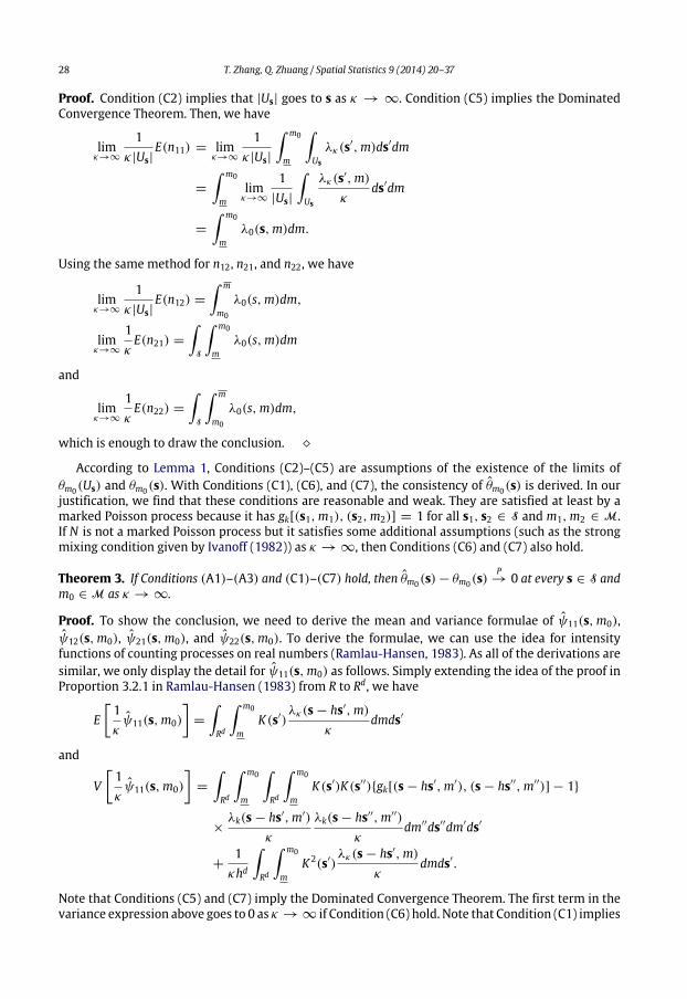
which is enough to draw the conclusion.
According to Lemma 1, Conditions (C2)–(C5) are assumptions of the existence of the limits ofθm0(Us) and θm0(s). With Conditions (C1), (C6), and (C7), the consistency of θm0(s) is derived. In ourjustification, we find that these conditions are reasonable and weak. They are satisfied at least by amarked Poisson process because it has gk[(s1,m1), (s2,m2)] = 1 for all s1, s2 ∈ S and m1,m2 ∈ M.If N is not a marked Poisson process but it satisfies some additional assumptions (such as the strongmixing condition given by Ivanoff (1982)) as κ → ∞, then Conditions (C6) and (C7) also hold.
Theorem 3. If Conditions (A1)–(A3) and (C1)–(C7) hold, then θm0(s)− θm0(s)P
→ 0 at every s ∈ S andm0 ∈ M as κ → ∞.
Proof. To show the conclusion, we need to derive the mean and variance formulae of ψ11(s,m0),ψ12(s,m0), ψ21(s,m0), and ψ22(s,m0). To derive the formulae, we can use the idea for intensityfunctions of counting processes on real numbers (Ramlau-Hansen, 1983). As all of the derivations aresimilar, we only display the detail for ψ11(s,m0) as follows. Simply extending the idea of the proof inProportion 3.2.1 in Ramlau-Hansen (1983) from R to Rd, we have
E1κψ11(s,m0)
=
Rd
m0
mK(s′)
λκ(s − hs′,m)κ
dmds′
and
V1κψ11(s,m0)
=
Rd
m0
m
Rd
m0
mK(s′)K(s′′)gk[(s − hs′,m′), (s − hs′′,m′′)] − 1
×λk(s − hs′,m′)
κ
λk(s − hs′′,m′′)
κdm′′ds′′dm′ds′
+1κhd
Rd
m0
mK 2(s′)
λκ(s − hs′,m)κ
dmds′.
Note that Conditions (C5) and (C7) imply the Dominated Convergence Theorem. The first term in thevariance expression above goes to 0 as κ → ∞ if Condition (C6) hold. Note that Condition (C1) implies
K(s′) is bounded. The second term goes to 0 as κ → ∞ if Conditions (C1) and (C5) hold. Note thatCondition (C1) also implies the integrand in mean expression above goes to λ0(s,m) for any fixeds′ ∈ S. With Conditions (C4) and (C5), we have
1κψ11(s,m0)
P→
Rd
m0
mK(s′)λ0(s,m)dmds′ =
m0
mλ0(s,m)dm.
Similarly, we can show
1κψ12(s,m0)
P→
m
m0
λ0(s,m)dm.
These two equations also imply the second term in (10) or (11) goes to zero in probability. Therefore,it is enough to focus on the first term in (10) or (11). Using the same method, we have
1κψ21(m0)
P→
Rd
m0
mλ0(s,m)dmds
and
1κψ22(m0)
P→
Rd
m
m0
λ0(s,m)dmds.
Using the Continuous Mapping Theorem, we have θm0(s)− θm0(s)P
→ 0 at everym0 and s.
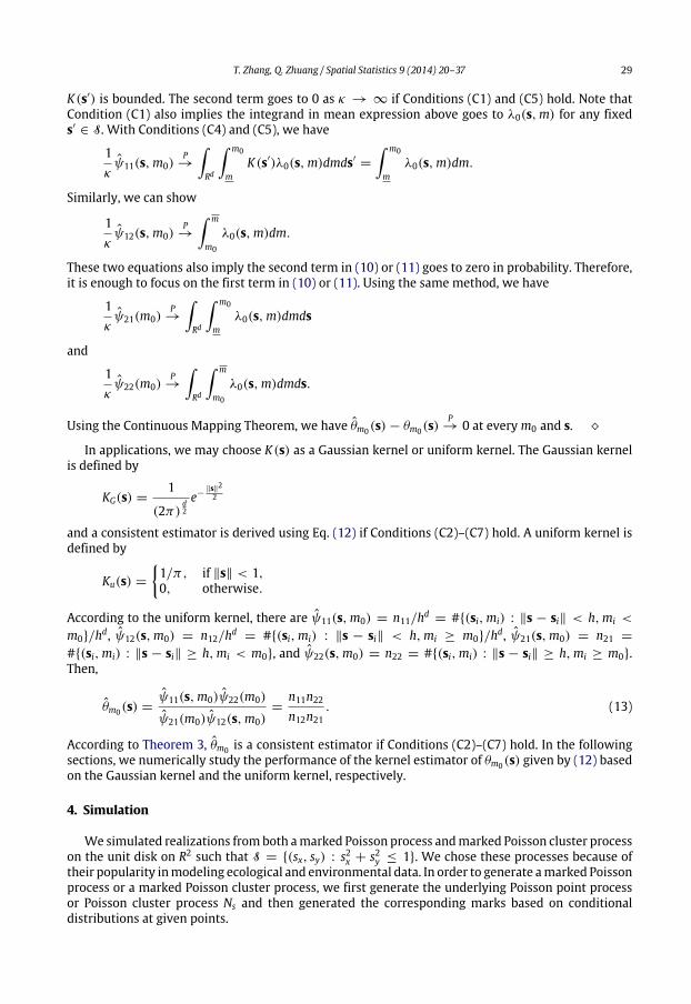
In applications, we may choose K(s) as a Gaussian kernel or uniform kernel. The Gaussian kernelis defined by
KG(s) =1
(2π)d2e−
∥s∥22
and a consistent estimator is derived using Eq. (12) if Conditions (C2)–(C7) hold. A uniform kernel isdefined by
Ku(s) =
1/π, if ∥s∥ < 1,0, otherwise.
According to the uniform kernel, there are ψ11(s,m0) = n11/hd= #(si,mi) : ∥s − si∥ < h,mi <
According to Theorem 3, θm0 is a consistent estimator if Conditions (C2)–(C7) hold. In the followingsections, we numerically study the performance of the kernel estimator of θm0(s) given by (12) basedon the Gaussian kernel and the uniform kernel, respectively.
4. Simulation
We simulated realizations fromboth amarked Poisson process andmarked Poisson cluster processon the unit disk on R2 such that S = (sx, sy) : s2x + s2y ≤ 1. We chose these processes because oftheir popularity inmodeling ecological and environmental data. In order to generate amarked Poissonprocess or a marked Poisson cluster process, we first generate the underlying Poisson point processor Poisson cluster process Ns and then generated the corresponding marks based on conditionaldistributions at given points.
For both processes, the first-order intensity function of Ns was defined as
λa(s) =
κae−a∥s∥2/[π(1 − e−a)], if a > 0,κ/π, if a = 0,
(14)
provided ∥s∥ ≤ 1, where κ was pre-selected constant. We chose the above model because it yieldedE[Ns(S)] = κ , which made the point density as
fa(s) = λa(s)/κ.To successfully generate the underlying Ns, for marked Poisson process, we generated homogeneousPoisson process on S with the intensity function equal to λa(s) = λa(s)a/(1 − e−a). As long aspoints were derived, each point was then thinned with the retained probability equal to e−a∥s∥ whichproduced a Poisson point Ns with intensity λa(s). For the marked Poisson cluster process, we firstgenerated homogeneous parent processwith intensity function equal to λa(s)/k. As long as the parentprocess was derived, we generated the offspring process according to the rule of Poisson clusterprocess (Diggle et al., 2003): the number of offspring points corresponding to each parent pointfollowed a Poisson distribution with mean k and the position of each offspring relative to its parentwas defined as a radial symmetric Gaussian random variable with standard deviation σ . We choseσ = 0.02. After that, each offspring was then thinned according to the samemethod that we used forthe marked Poisson process. Therefore in both cases, we had the first-order intensity function of Nsequal to λa(s) given by Eq. (14). As long as points were derived, we generated marks independentlyfrom N(ν, 1) distribution with
ν = ν(s) = η(1 − ∥s∥), η ≥ 0. (15)It was clear that both stationary and nonstationary Ns could be generated respectively according toEqs. (14) and (15): a stationary Ns was derived if a = 0 and a nonstationary Ns was derived if a = 0.As long as points were derived, we had θm0(s) = 1 for anym0 and s if and only if η = 0.
According to the statisticalmodel in our simulation,we hadψ11(s,m0) = Φ[m0−η(1−∥s∥)]λa(s),ψ12(s,m0) = 1 − Φ[m0 − η(1 − ∥s∥)]λa(s). If a = 0, then
1κψ21(m0) =
11 − e−a
[Φ(m0 − η)− e−aΦ(m0)]
+ηe
−a(m0−η)2
η2+2a
(1 − e−a)η2 + 2a
Φ
η2 + 2a
1 +
η(m0 − η)
η2 + 2a
− Φ
η(m0 − η)η2 + 2a
and
1κψ22(m0) =
11 − e−a
[(1 − e−a)+ Φ(m0)e−a− Φ(m0 − η)]
−ηe
−a(m0−η)2
η2+2a
(1 − e−a)η2 + 2a
Φ
η2 + 2a
1 +
η(m0 − η)
η2 + 2a
− Φ
η(m0 − η)η2 + 2a
.
If a = 0, then1κψ21(m0) = Φ(m0)−
1η2
[1 + (η − m0)
2][Φ(m0)− Φ(m0 − η)]
+η − m0√2π
e−(m0−η)2
2 +m0 − 2η
√2π
e−m202
and
1κψ22(m0) = [1 − Φ(m0)] +
1η2
[1 + (η − m0)
2][Φ(m0)− Φ(m0 − η)]
+η − m0√2π
e−(m0−η)2
2 +m0 − 2η
√2π
e−m202
.
Therefore, the value of θm0(s) could be analytically derived.
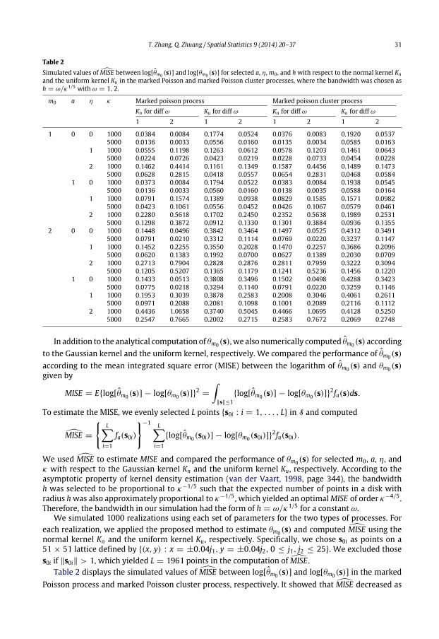
Table 2Simulated values of MISE between log[θm0 (s)] and log[θm0 (s)] for selected a, η,m0 , and hwith respect to the normal kernel Knand the uniform kernel Ku in the marked Poisson and marked Poisson cluster processes, where the bandwidth was chosen ash = ω/κ1/5 with ω = 1, 2.
m0 a η κ Marked poisson process Marked poisson cluster processKn for diff ω Ku for diff ω Kn for diff ω Ku for diff ω1 2 1 2 1 2 1 2
In addition to the analytical computation of θm0(s), we also numerically computed θm0(s) accordingto the Gaussian kernel and the uniform kernel, respectively. We compared the performance of θm0(s)according to the mean integrated square error (MISE) between the logarithm of θm0(s) and θm0(s)given by
MISE = Elog[θm0(s)] − log[θm0(s)]2
=
∥s∥≤1
log[θm0(s)] − log[θm0(s)]2fa(s)ds.
To estimate the MISE, we evenly selected L points s0i : i = 1, . . . , L in S and computed
MISE =
L
i=1
fa(s0i)
−1 Li=1
log[θm0(s0i)] − log[θm0(s0i)]2fa(s0i).
We used MISE to estimate MISE and compared the performance of θm0(s) for selected m0, a, η, andκ with respect to the Gaussian kernel Kn and the uniform kernel Ku, respectively. According to theasymptotic property of kernel density estimation (van der Vaart, 1998, page 344), the bandwidthh was selected to be proportional to κ−1/5 such that the expected number of points in a disk withradius hwas also approximately proportional to κ−1/5, which yielded an optimalMISE of order κ−4/5.Therefore, the bandwidth in our simulation had the form of h = ω/κ1/5 for a constant ω.
We simulated 1000 realizations using each set of parameters for the two types of processes. Foreach realization, we applied the proposed method to estimate θm0(s) and computed MISE using thenormal kernel Kn and the uniform kernel Ku, respectively. Specifically, we chose s0i as points on a51 × 51 lattice defined by (x, y) : x = ±0.04j1, y = ±0.04j2, 0 ≤ j1, j2 ≤ 25. We excluded thoses0i if ∥s0i∥ > 1, which yielded L = 1961 points in the computation of MISE.
Table 2 displays the simulated values of MISE between log[θm0(s)] and log[θm0(s)] in the markedPoisson process and marked Poisson cluster process, respectively. It showed that MISE decreased as
κ increased. This was expected because a larger κ value indicated a more precise estimate of θm0(s).The values of MISE were significantly affected bym0, η and ω. We compared the performance of MISEbetween marked Poisson process and marked Poisson cluster process as well as the values of a andfound that values of MISE were close. Therefore, we concluded that the performance of θm0(s) wassignificantly affected by the first-order property but not by the second-order property of Ns. In thecomparison between kernel functions, we found that the performance of Gaussian kernel was betterif ηwas small (i.e. η = 0) butworse if ηwas large (i.e. η = 2). Althoughwe could not general concludewhich kernel function should be better used in applications, wemight conclude that the performanceof uniform kernel was better if point patterns were inhomogeneous. Overall, we concluded that theinfluence of m0, η, κ , bandwidth, and kernel functions was substantial but the dependence betweenpoints in Ns was not.
5. Case study
We applied our approach to the Alberta Forest Wildfire data and the Japan Earthquake data. Usingthe method proposed by Schoenberg (2004) for testing independence between points and marks, wefound that the independence between points andmarks was rejected in both datasets. The result wasnot displayed in this article as it was not the interest in our data analysis. In the Alberta Forest Wildfiredata, we chose m0 = 2 km2 as a forest wildfire is called large if the area burned is greater than orequal to 2 km2. In the Japan Earthquake data, we chose m0 = 6 because an earthquake is often calledlarge if the magnitude is greater than or equal to 6. As long as m0 was decided, we used the Gaussiankernel Kn and the uniform kernel Ku to compute θm0(s). As long as θm0(s)was derived, we used θm0(s)to interpret the relationship between points and marks. According to the definition of θm0(s), it isrecommended to pay much attention to subregions with low values of θm0(s).
5.1. Alberta forest wildfire data
The Alberta Forest Wildfire data consisted of forest wildfire activities in Alberta, Canada, from 1931to 2012. The Canadian Alberta Forest Service initiated the modern era of wildfire record keeping in1931. Over the years, this fire information has been recorded, stored and made available in differentformats. Beginning in 1996, paper copies of wildfire historical information were no longer retained.Thewildfire historical data were entered at the field level on the Fire Information Resource EvaluationSystem (FIRES), which are available at http://www.srd.alberta.ca/Wildfire.
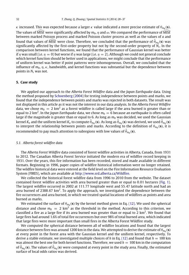
We collected the historical forest wildfire data from 1996 to 2010 from the website. The datasetcontained forest wildfire activities with area burned greater than or equal to 0.01 hectares (Fig. 1).The largest wildfire occurred in 2002 at 111.77 longitude west and 55.47 latitude north and had anarea burned of 2388.67 km2. To apply the approach, we investigated the dependence between thefire occurrences and area burned, in which we treated spatial locations of wildfires as points and areaburned as marks.
We estimated the surface of θm0(s) by the kernel method given in Eq. (12). We used the sphericaldistance and chose m0 = 2 km2 as the threshold in the method. According to this criterion, weclassified a fire as a large fire if its area burned was greater than or equal to 2 km2. We found thatlarge fires had around 1.6% of total fire occurrences but over 98% of total burned area, which indicatedthat large fires were more important than small fires in the Alberta Forest Wildfire study.
We computed the spherical distance between all of wildfire locations and found that the largestdistance between fireswas around 1200 km in the data.We attempted to derive the estimate of θm0(s)at every point in the forest area with the Gaussian kernel and the uniform kernel, respectively. Toderive a stable estimate, we investigated multiple choices of h in Eq. (12) and found that h = 100 kmwas almost the best one for both kernel functions. Therefore, we used h = 100 km in the computationof θm0(s). The values of θm0(s)were computed at every point in the study area. Finally, the estimatedsurface of local odds ratios was derived.
Fig. 1. Wildfire locations in Alberta forest wildfire data.
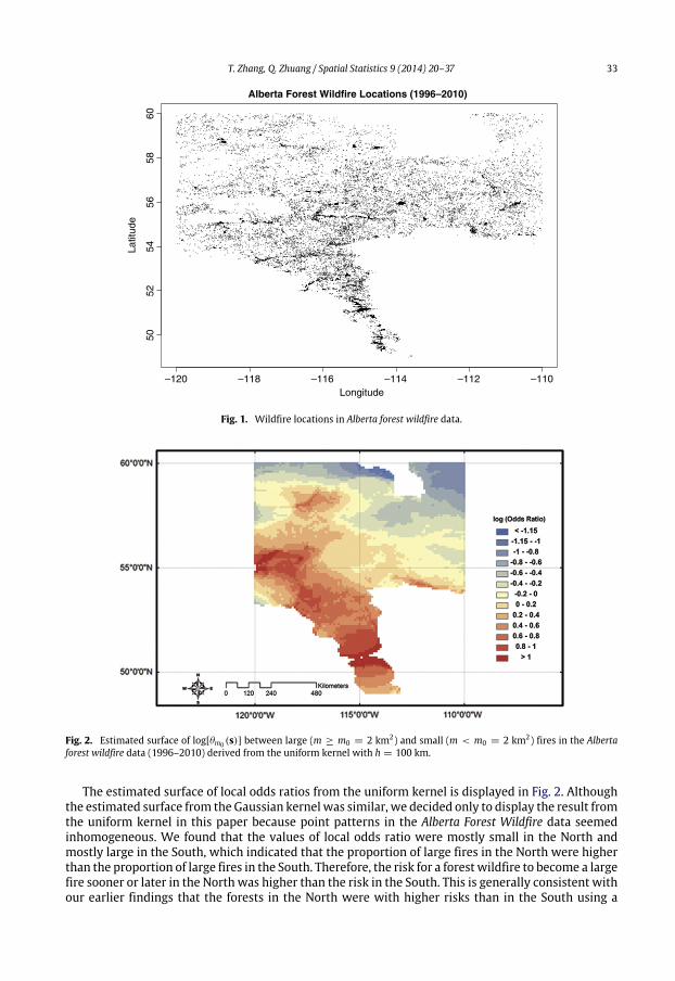
Fig. 2. Estimated surface of log[θm0 (s)] between large (m ≥ m0 = 2 km2) and small (m < m0 = 2 km2) fires in the Albertaforest wildfire data (1996–2010) derived from the uniform kernel with h = 100 km.
The estimated surface of local odds ratios from the uniform kernel is displayed in Fig. 2. Althoughthe estimated surface from the Gaussian kernelwas similar, we decided only to display the result fromthe uniform kernel in this paper because point patterns in the Alberta Forest Wildfire data seemedinhomogeneous. We found that the values of local odds ratio were mostly small in the North andmostly large in the South, which indicated that the proportion of large fires in the North were higherthan the proportion of large fires in the South. Therefore, the risk for a forest wildfire to become a largefire sooner or later in the North was higher than the risk in the South. This is generally consistent withour earlier findings that the forests in the North were with higher risks than in the South using a
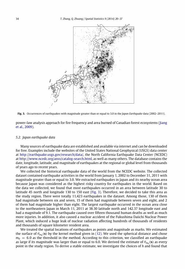
Fig. 3. Occurrences of earthquakes with magnitude greater than or equal to 3.0 in the Japan Earthquake data (2002–2011).
power-law analysis approach for fire frequency and area burned of Canadian forest ecosystems (Jianget al., 2009).
5.2. Japan earthquake data
Many sources of earthquake data are established and available via internet and can be downloadedfor free. Examples include the websites of the United States National Geophysical (USGS) data centerat http://earthquake.usgs.gov/research/data/, the North California Earthquake Data Center (NCEDC)at http://www.ncedc.org/anss/catalog-search.html, as well as many others. The database contains thedate, longitude, latitude, andmagnitude of earthquakes at the regional or global level from thousandsof years ago to recent years.
We collected the historical earthquake data of the world from the NCEDC website. The collecteddataset contained earthquake activities in the world from January 1, 2002 to December 31, 2011 withmagnitude greater than or equal to 3.0. We extracted earthquakes in Japan and its nearby ocean areabecause Japan was considered as the highest risky country for earthquakes in the world. Based onthe data we collected, we found that most earthquakes occurred in an area between latitude 30 tolatitude 45 north and longitude 130 to 150 east (Fig. 3). Therefore, we decided to take this area asthe study region. There were totally 11,423 earthquakes in the dataset. Among those, 130 of themhad magnitude between six and seven, 15 of them had magnitude between seven and eight, and 2of them had magnitude higher than eight. The largest earthquake occurred in the ocean area closeto the northeastern Japan in March 11, 2011 at 38.30 latitude north and 142.37 longitude east andhad a magnitude of 9.1. The earthquake caused over fifteen thousand human deaths as well as muchmore injuries. In addition, it also caused a nuclear accident of the Fukushima Daiichi Nuclear PowerPlant, which induced a huge leak of nuclear radiation affecting hundreds of thousands of residentsand thousands of square kilometer resident area.
We treated the spatial locations of earthquakes as points and magnitude as marks. We estimatedthe surface of θm0(s) by the kernel method given in (12). We used the spherical distance and chosem0 = 6.0 as the threshold in the method. According to this criterion, we classified an earthquakeas large if its magnitude was larger than or equal to 6.0. We derived the estimate of θm0(s) as everypoint in the study region. To derive a stable estimate, we investigate the choices of h and found that
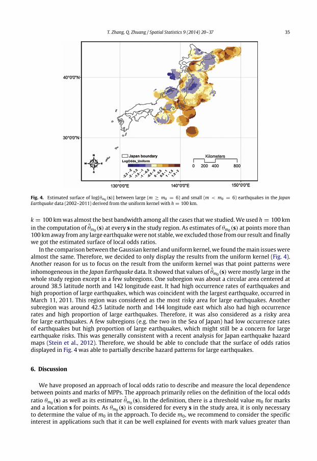
Fig. 4. Estimated surface of log[θm0 (s)] between large (m ≥ m0 = 6) and small (m < m0 = 6) earthquakes in the JapanEarthquake data (2002–2011) derived from the uniform kernel with h = 100 km.
k = 100 kmwas almost the best bandwidth among all the cases thatwe studied.We used h = 100 kmin the computation of θm0(s) at every s in the study region. As estimates of θm0(s) at points more than100 kmaway fromany large earthquakewere not stable,we excluded those fromour result and finallywe got the estimated surface of local odds ratios.
In the comparison between theGaussian kernel and uniformkernel,we found themain issueswerealmost the same. Therefore, we decided to only display the results from the uniform kernel (Fig. 4).Another reason for us to focus on the result from the uniform kernel was that point patterns wereinhomogeneous in the Japan Earthquake data. It showed that values of θm0(s)were mostly large in thewhole study region except in a few subregions. One subregion was about a circular area centered ataround 38.5 latitude north and 142 longitude east. It had high occurrence rates of earthquakes andhigh proportion of large earthquakes, which was coincident with the largest earthquake, occurred inMarch 11, 2011. This region was considered as the most risky area for large earthquakes. Anothersubregion was around 42.5 latitude north and 144 longitude east which also had high occurrencerates and high proportion of large earthquakes. Therefore, it was also considered as a risky areafor large earthquakes. A few subregions (e.g. the two in the Sea of Japan) had low occurrence ratesof earthquakes but high proportion of large earthquakes, which might still be a concern for largeearthquake risks. This was generally consistent with a recent analysis for Japan earthquake hazardmaps (Stein et al., 2012). Therefore, we should be able to conclude that the surface of odds ratiosdisplayed in Fig. 4 was able to partially describe hazard patterns for large earthquakes.
6. Discussion
We have proposed an approach of local odds ratio to describe and measure the local dependencebetween points and marks of MPPs. The approach primarily relies on the definition of the local oddsratio θm0(s) as well as its estimator θm0(s). In the definition, there is a threshold value m0 for marksand a location s for points. As θm0(s) is considered for every s in the study area, it is only necessaryto determine the value of m0 in the approach. To decide m0, we recommend to consider the specificinterest in applications such that it can be well explained for events with mark values greater than
and less thanm0, respectively. Whenm0 is decided, the estimated value θm0(s) at every s in the studyarea forms an estimate of the surface of local odds ratios.
According to its definition, the local odds ratio is the ratio of the odds between small and largeevents at the local level to the global level. It is also equal to the ratio of the relative risk of smallevents to the relative risks of large events. The value of the local odds ratio describes the risk for anevent to finally become large at the local level relative to the global level. The ratio of two local oddsratios describes the risk of large events between the two specific locations. Therefore, the surface oflocal odds ratios may be used as an index measure for the risk of an event to become a large event inthe end conditioning on the observation of an event.
We expect that the proposed approach will find wide applications in natural hazards studies, asmany important issues can be discovered by studying the estimated surface of local odds ratios. Forexample, in a forest wildfire study, if the value of local odds ratio is low, then as long as a fire isobserved at the beginning it is more likely for the fire to be large in the end. In an earthquake study,if the value of local odds ratio is low, then energy accumulated is less likely to be released by manysmall earthquakes rather than by a few large earthquakes. Therefore, our approach suggests that riskstudies should pay more attention to the area that has small local odds ratios.
There are a few possible extensions to the approach. First, the local odds ratio defined in thisarticle only involves the first-order intensity function, which cannot be used to interpret higher-orderdependence between points andmarks. Second, even though we have provided a method to estimatethe local odds ratio, we have not considered any explanatory variables. It will be important to developa method that models the local odds ratio by explanatory variables (e.g., in forest fire studies, theeffects of drought condition and fuel loadings). Third, according to the definition, the local odds ratioonly involves the odds between events with mark values higher than and lower than a threshold. Itcannot be directly used to analyze the dependence between points and marks if two or more criticalthreshold values are considered. To extend our proposed approach by considering the above issueswill be important to wide applications and deserves further investigations.
Acknowledgments
This research is partly supported by the NASA Land Use and Land Cover Change program (NASA-NNX09AI26G), Department of Energy (DE-SC0007007), the United StatesNSF-Division of Informationand Intelligent Systems (NSF-1028291). The authors appreciate suggestive comments from twoanonymous referees which significantly improve the quality of the paper.
References
Agresti, A., 2002. Categorical Data Analysis. Wiley, New York.Baddeley, A., Turner, R., 2005. spatstat: an R package for analyzing spatial point patterns. J. Statist. Softw. 12, 1–42.Cressie, N., 1993. Statistics for Spatial Data. Wiley, New York.Daley, D.J., Vere-Jones, D., 2003. An Introduction to Theory of Point Processes: Volume I: Elementary Theory and Methods,
second ed.. Springer, New York.Diggle, P.J., Ribeiro, J.P.J., Christensen, O., 2003. An introduction tomodel-based geostatistics. In:Moller, J. (Ed.), Spatial Statistics
and Computational Methods, Springer, New York, pp. 43–86.Guan, Y., Afshartous, D.R., 2007. Test for independence between marks and points of marked point processes: a subsampling
approach. Environ. Ecol. Stat. 14, 101–111.Harte, D., 2010. PtProcess: an R Package for modelling marked point processes indexed by time. J. Statist. Softw. 35, 1–32.Ho, L.P., Stoyan, D., 2008. Modeling marked point patterns by intensity-marked Cox processes. Statist. Probab. Lett. 78,
2831–2842.Holden, L., Sannan, S., Bungum, H., 2003. A stochastic marked point process model for earthquakes. Nat. Haz. Earth Syst. Sci. 3,
95–101.Ivanoff, G., 1982. Central limit theorems for point processes. Stochastic Process. Appl. 12, 171–186.Jiang, Y., Zhuang, Q., Flannigan, M.D., Little, J.M., 2009. Characterization of wildfire regimes in Canadian boreal terrestrial
ecosystems. Internat. J. Wildland Fire 18, 992–1002.Karr, A.F., 1991. Point Processes and their Statistical Inference, second ed. Marcel Dekker, Inc., New York.Malamud, B.D., Millington, J.D.A., Perry, G.L.W., 2005. Characterizing wildfire regimes in the United States. In: Proceedings of
the National Academy of Sciences of the United States of America, vol. 102, pp. 4694–4699.Malinowski, A., Schlather, M., Zhang, Z., 2012. Intrinsically weighted means of marked point processes. Arxiv:1201.1335.McElroy, T., Politis, D.N., 2007. Stable marked point processes. Ann. Statist. 35, 393–419.Moller, J., Waagepetersen, R., 2007. Modern statistics for spatial point processes. Scand. J. Statist. 34, 643–684.
Myllymäki, M., Penttinen, A., 2009. Conditionally heteroscedastic intensity-dependent marking of log Gaussian Cox processes.Stat. Neerl. 63, 450–473.
Ogata, Y., 1988. Statistical models for earthquake occurrences and residual analysis for point processes. J. Amer. Statist. Assoc.83, 9–27.
Ogata, Y., Katsura, K., 1993. Analysis of temporal and spatial heterogeneity of magnitude frequency distribution inferred fromearthquake catalogs. Geophys. J. Internat. 113, 727–738.
Ogata, Y., 1998. Space–time point process models for earthquake occurrences. Ann. Institut. Statist. Math. 50, 379–402.Peng, R.D., Schoenberg, F.P, Woods, J.A., 2005. A space–time conditional intensity model for evaluating a wildfire hazard index.
J. Amer. Statist. Assoc. 100, 26–35.Poliltis, D.N., Sherman, M., 2001. Moment estimation for statistics from marked point processes. J. Roy. Statist. Soc. Ser. B 63,
261–275.Ramlau-Hansen, R., 1983. Smoothing counting process intensities by means of kernel functions. Ann. Statist. 2, 453–466.Schlather, M., Ribeiro, P.J., Diggle, P.J., 2004. Detecting dependence between marks and locations of marked point processes.
J. Roy. Statist. Soc. Ser. B 66, 79–93.Schoenberg, F.P., 2004. Testing separability in spatial–temporal marked point processes. Biometrics 60, 471–481.Stein, A., Van Lieshout, M.N.M., Booltink, H.W.G., 2011. Spatial interaction of methylene blue stained soil pores. Geoderma 102,
101–121.Stein, S., Geller, R.J., Liu, M., 2012. Why earthquake hazard maps often fail and what to do about it. Tectonophysics 562–563,
1–25.van der Vaart, A.W., 1998. Asymptotic Statistics. Cambridge University Press, Cambridge, UK.Vere-Jones, D., 1995. Statistical methods for the description and display of earthquake catalogs. In: Walden, A., Guttorp, P.
(Eds.), Statistics in Environmental and Earth Sciences. Edward Arnold, London, pp. 220–236.