Third SPE Comparative Project: Gas Cycling of Condensate Reservoirs Douglas E. Kenyon, SPE, Marathon Oil Co. G. Alda Behie, SPE, Dynamic Reservoir Systems Solution Retrograde 5w /2’279 Summary. Nhe companies participated in WISartificial modeling study of gas cycling in a rich retrograde- gas-condensate reservoir. .%rfaw oil rate pmdctions dWer in the esrly years of cycling but agree better late in cycling. The smount of condensate precipitated near the production well mrd ita rate of evaporation varied widely emong pa~lcipants. The explrmation appesrs to be in K-value techniques used. Prccomputcd tables for K values produced rapid and thorough removsl of condensate during later years of cycling. Equation-of-ststc (EOS) methods produced a stabilized condensate asturation sufficient to flow liquid during the greater part of cycfing, and the condensate never completely revaporized. We do not know which prdlction is more nearly correct because our PVT data d]d not cover the rsnge of compositions that exists in tfrk srea of the reservoir model. lntroduotion SPE conducted two earlier solution projccta, [32both de- signed to measure the state-of-tie-art simulation capabilhy for challenging and timely modeling problems. The fmt project involved a three-layer black-oil simulation with gas injection into the top layer. 1 Both constant and vari- able bubblepoint pressure assumptions were used. Model prdctions were in fsir agreement. No simnlator perform- ance &ta (mn times, timestep size, etc.) were given. Seven companies participated in the project. The second project was a study of water and gaa coning with a radial grid and 15 layers. 2 Authors of the project fek that un- usrxd well rate variations and a high assumed solution 00R contributed to the dit%cuky of the problem. Some significant dkcrepancies in oil rate snd pressure were ob- tained. Eleven compsnies joined in the project. For the thkd comparative solution project, the Com- mittee for the Numerical Simulation Symposium sought a compositional modeling probtem. Numerical compari- sons of the PVT data match were considered important. Speed of the simulators was not to be of major interest. The problem we designed is the outcome of this fsirly general request. Some features of interest in current pro- duction pracdce of pressure maintenance by gas injection are included. The results confirm the well-kqown trade- off between the timing of gas sales and tie amount of con- densate recovered. Seversl features of intereat in a more complete examination of production from gas-condensate resewoirs are ignored. These include the effects of ncaf- well liquid saturation buildup on well productivity and of water encroachment and water production on hydrocar- bon productivity. We did not address the role of numeri- Cd dkpe:sion. Irr addition, the surface process is simplified and not representative of economical liquid recovery in typical offshore operations. We simplified the surface process to attract a larger number of participants. CWYrighx19S7sway of PeUolmnE.ginem Journal of Perrdemn Technology, A.SIM 1987 because not aUcompanies had facilities for simulating gas plant processing with gas recycling in their composition- al simulators. Nine compmries responded to the invitation forpartici- pation. Table I is a list of the participants in thk project. Participant responses were well prepared and required a minimum of discussion. We invited all the companies to use as msny components as neceassry for rhe accurate match of the PVT date snd for the simulation of gsa cy- cling. Companies were asked to give components actually used in the reservoir model, how these components were chafacterizcd, and the match to the PVT data obtained wim the components. We first outline the problem specifications, including sufficient data for others who may wish to try the prob- lem. The pertinent PVT datn are given. We show each participant’a components, the properties of these compo- nent, and the basic PVT match obtained. In many cases, EOS methods were used exclusively, but in others, a com- bmtion of methods was applied. The results of the reser- voir simulation are given and comparisons nre shown between companies for both cycliig-smategy cases. Fi- nally, some facts regardhrg simulator performance are given, sltbough tids information waa voluntary. Problem Statement The two major parts to a compositional model study are the PVT data and the reservoir grid. For the PVT data, participants were supplied with a companion set of fluid analysis reports. The specification of the reservoir model is given in Tables 2 snd 3 and the grid is shown in Fig. 1. Note that the grid is 9 X9 X4 end symmetrical, indicat- ing that it would be possible to simulate half the ideated grid. Most participants chose to model the fufl @d. Note slso that the layers sre homogeneous and of constant porosity, but that permeability end thickrress vary among layers. 981
Transcript
Third SPE ComparativeProject: Gas Cycling ofCondensate ReservoirsDouglas E. Kenyon, SPE, Marathon Oil Co.G. Alda Behie, SPE, Dynamic Reservoir Systems
SolutionRetrograde
5 w /2’279
Summary. Nhe companies participated in WISartificial modeling study of gas cycling in a rich retrograde-gas-condensate reservoir. .%rfaw oil rate pmdctions dWer in the esrly years of cycling but agree better latein cycling. The smount of condensate precipitated near the production well mrd ita rate of evaporation variedwidely emong pa~lcipants. The explrmation appesrs to be in K-value techniques used. Prccomputcd tables forK values produced rapid and thorough removsl of condensate during later years of cycling. Equation-of-ststc(EOS) methods produced a stabilized condensate asturation sufficient to flow liquid during the greater part ofcycfing, and the condensate never completely revaporized. We do not know which prdlction is more nearlycorrect because our PVT data d]d not cover the rsnge of compositions that exists in tfrk srea of the reservoirmodel.
lntroduotion
SPE conducted two earlier solution projccta, [32both de-signed to measure the state-of-tie-art simulation capabilhyfor challenging and timely modeling problems. The fmtproject involved a three-layer black-oil simulation withgas injection into the top layer. 1 Both constant and vari-able bubblepoint pressure assumptions were used. Modelprdctions were in fsir agreement. No simnlator perform-ance &ta (mn times, timestep size, etc.) were given.Seven companies participated in the project. The secondproject was a study of water and gaa coning with a radialgrid and 15 layers. 2 Authors of the project fek that un-usrxd well rate variations and a high assumed solution00R contributed to the dit%cuky of the problem. Somesignificant dkcrepancies in oil rate snd pressure were ob-tained. Eleven compsnies joined in the project.
For the thkd comparative solution project, the Com-mittee for the Numerical Simulation Symposium soughta compositional modeling probtem. Numerical compari-sons of the PVT data match were considered important.Speed of the simulators was not to be of major interest.
The problem we designed is the outcome of this fsirlygeneral request. Some features of interest in current pro-duction pracdce of pressure maintenance by gas injectionare included. The results confirm the well-kqown trade-off between the timing of gas sales and tie amount of con-densate recovered. Seversl features of intereat in a morecomplete examination of production from gas-condensateresewoirs are ignored. These include the effects of ncaf-well liquid saturation buildup on well productivity and ofwater encroachment and water production on hydrocar-bon productivity. We did not address the role of numeri-Cd dkpe:sion. Irr addition, the surface process issimplified and not representative of economical liquidrecovery in typical offshore operations. We simplified thesurface process to attract a larger number of participants.
CWYrighx19S7sway of PeUolmnE.ginem
Journal of Perrdemn Technology, A.SIM 1987
because not aUcompanies had facilities for simulating gasplant processing with gas recycling in their composition-al simulators.
Nine compmries responded to the invitation forpartici-pation. Table I is a list of the participants in thk project.Participant responses were well prepared and required aminimum of discussion. We invited all the companies touse as msny components as neceassry for rhe accuratematch of the PVT date snd for the simulation of gsa cy-cling. Companies were asked to give components actuallyused in the reservoir model, how these components werechafacterizcd, and the match to the PVT data obtainedwim the components.
We first outline the problem specifications, includingsufficient data for others who may wish to try the prob-lem. The pertinent PVT datn are given. We show eachparticipant’a components, the properties of these compo-nent, and the basic PVT match obtained. In many cases,EOS methods were used exclusively, but in others, a com-bmtion of methods was applied. The results of the reser-voir simulation are given and comparisons nre shownbetween companies for both cycliig-smategy cases. Fi-nally, some facts regardhrg simulator performance aregiven, sltbough tids information waa voluntary.
Problem Statement
The two major parts to a compositional model study arethe PVT data and the reservoir grid. For the PVT data,participants were supplied with a companion set of fluidanalysis reports. The specification of the reservoir modelis given in Tables 2 snd 3 and the grid is shown in Fig.1. Note that the grid is 9 X9 X4 end symmetrical, indicat-ing that it would be possible to simulate half the ideatedgrid. Most participants chose to model the fufl @d. Noteslso that the layers sre homogeneous and of constantporosity, but that permeability end thickrress vary amonglayers.
981
TABLE1–COMPANIES PARTICIPATING IN THIRDSPE COMPARATIVE SOLUTION PROJECT
Arco oil and Gas Co.P.O. BOX 2819Dallas, TX 75221
Chevron Oil Field Research CO.P.O. BOX 446La Habra, CA90631Core Laboratories Inc.7600 Carpenter FreewayP.O. Box 47547Dallas, TX 75247
Computer ModelfingGTUP (CMG)3512-33 Street N.W.Calgary, Alta.Canada T2L 2A6
Sot. Natl. Elf Aquitaine26, Avenue des Lilas64018 Pau CedexFrance
Intercomp’1801 California St.Fourth FloorDenver, CO 80202-2699
Marathon Oil Co.P.O. BOX 269LitOeton, CO 80160-0269
McCord-Lewis Energy SewicesP.O. Box 453o7Oallas, TX 75245
Petek, The Petroleum Technology Research Inst.N-7034 Tmndheim NTHNorway
.NowScientificSoltwar&n,,rcomP,
7330f!7360<,7400ii
—-----l/ .,450 ‘t
— D&TUM.7500 ?1(,. bs.rfm,]
‘h----.kINJECTION PRODUCTION
COMPLETIONS COMPLETIONS
‘i9. 1—Thi rd comparative solution project 9 xs x 4 reser.oir model grid.
982
TASLE 2—RESERVOIR GRID ANO SATURATIONINPUT DATA
Resewoir Grid Data
NX=NY=9, NZ=4DX = DY=293.3 ftDatum (subsurface), ft 7,500Porosity (at initial reservoir pressure) 0.13Gas/water contact, ft 7,500Water saturation at 60nt20t ,1.00Capillary pressure at contact, psiInitial pressure at comzct, psia 3,55:Water properties
density at contqct, lbm/ft3 63.0compre33ibiiity, psi -‘ 3.0 XIO-6
The grid size sets the value of numerical dispersion inthese implicit pressure, explicii saturation flMPES)models. The grid size selected represents a reasombIe gridfor,certain offshore applications but is somewhat too re-fined for a full-field simulation. The producer is not inthe very comer of the grid. Most of tie area behind theproducer undergoes pressuie depletion only because it isnot swept by injection gas. In thk area, retrograde con-densation occurs without significant evapora.tiop by recy-cle g8s to simulate areas of minim61 sweep in a realreservoir.
The initial conditions for the location of the gaslwakrcontact and the capillary pressure &ta generate a water/gas transition 2one exteding into the pay layer8.’Tbe verysmall compressib~lty aod volume of water, however,
Journal of Petroleum Tecknolow,August1987
make water rather insignificant for this problem. Relativep+mneabtity ckdswere based on the simplistic assumptionthat the relative permeability of 8ny phase depends onfyon its saturation. Note that condensate is immobile up to24% saturation and thst k,g is reduced fimfr 0.74 to 0.40as condensate builds to this saturation with irreduciblewater present.
Layer 1 is a high-pmneability layer (130 md) with rapidmovement of injected gas. The produced gas bscomes amix of reservoir gas with’ ‘dry.gas. ” The path of migra-tion of injected gas is along Layer 1 with a mm down-ward only in a smsff zone around the producer, whichis completed in Layers 3 sud 4. Layer 4 is also a hlgh-permeability layer (150 red), but our review of satum-tion srray data revealed that most of the injected gss thatreaches the producer in Layer 4 has come across Layer1 and turned downward as it approaches the producer.We speculate that buoyancy, high vertic61 permeability,and wme extra water in Layer 4 explsin the favored flowof dry gas through Layer 1.
Liquid production by multistage sepsmtion ia thetmknown to be predlctcd. The primary separator pressuredepends on reservoir pressore as given in TabIe 3. Pro-duction is controlled by a specified separator-gas rate. In-”jetted gsa is tsken from the combined vapor streams oftie fhree-stuge separation. Two cases were requested anddiffer by the recycIe-gsa rate assumed. Volume fricaJly,the two csaes provide for exsctly the same smount of recy-cle gas to be injcctcd over the duration of the cycling peri-od (10 years). Case 1 uses a constsnt recycle-gas rate(4,700 Mscf/D [133X 103 std m3/d]) for the entire cy-cling period. Case 2 uses a somewhat higher rste (5,700Mscf/D [161x103 std m3/d]) for the first 5 years of cy-cling and a somewhat lower rate (3,700 MscfiD[105 x 103 std m3/d]) for the last 5 ye.m of cycling.More gas is recycled in the criticsl early yews in Case2. This promotes pressure maintenance and incrcaaes sur-face liquid yieId (leas condensation in the reservoir) but
TABLE 3—WELL AND SEPARATOR INPUT DATA
Production, Injection, and Sales Dam
Production Well DataLocationI=J= 7Perforations K= 3, 4 (bottom layers)Radius, rw, If 1Rate (separator gas rate), Mscf/D 6,200Minimum bottomhole pressure, psi 500
Injection Well DafsLocation I=J= iPerforations K= 1, 2 (top layers)Radius, rw, If ‘1Rate (separator-gas rate minus saies-gas rate)Msximum bottomhole pressure, psi 4,000
Sales RateCase 1 (constant sales rate to blowdown)
0<1<10 years 1,500 Mscf/Dt>10 year% all produced gas to sales
Case 2 (defemed sales)0< tc5 years 500 Mscf/D5< t< 10 years 2,500 Mscf/Dt> 10 yea= all produced gas to sales
.Primaryseparatoratsl5 psiaunfitremrv.irpressure(atdatum)m w..v2,w m. w switcht..wimawseparalmal 315 psi..
reduces avtilable saks gas volume. Reservoir pressurefalls rapidly during fbe 16atyears of cycling in Case 2 andsurface liquid falk accordingly.
Blowdown (sll gas to salca) stats at the end of the I&hyear of cycling, and the modek were ron to 15 ycam or1,000-psi [6.9-MPa] average reservoir pressure, which-
I
I
TASLE 4—HYfJROCARBON ANALYSES OF SEPARATOR PRODUCTSANO CALCULATE WELL STREAM
Separator Liquid Separator Gas’ Well Stream
Component (mol %) (mol %) (gal/s.f x 103) (mol %) (gakcf x 103)
Measured PVT data are, given in Tables 4 through 15.The &ta include hydrocarbon sampIe analyses, wnstmt-composition expshsion data, constant-volume depletiondata, and swelling data of foui’ mixtures of reservoir gaswith lean gas.
Table 4 gives compositions of liquid and gas used tocreate a reservoir well-stream composition for depletion
934
TABLE 7—RETROGRADE CONDENSATION OURING5AS DEPLETION AT 2000F (Constant-Volume Depletion;
and swelling tests. UnIike most fluid analyses, theseparator-gas composition was prepared in the laboratorytitb pure components and not collected in the field. Fur-thermore, the separator liquid is a random condensatesample. These fluids were physically recombined at agasfliquid ratio of 4,812 scf/STB [857 std m3/stock-fankrn31. The resultant well-stream composition is correctlygiven in Table 4. Because gas and liquid samples usedfor recombination are not in equilibrium, however, thewell stream will not flash to the gas and liquid composi-tions of Table 4attbe indlatedpressure and tempera-ture. This peculiarity was spelled out in the cover letterof the fluid-analysis repmt sent to afl potential participants.
Table 5 gives more detail on the distribution of com-ponents intiesynthetic resavoirfluid. However, noneof the companies used this mrmy components for the PVTmatch.
Table 6 gives constant-composition expansion data, in-cludhg calculated Z. factors at and above the dewpointpressure. We wilf see later that all companies matchedthe relative volume in expansion accurately but that therewere some minor””dlfferences in calculated Zfactors.
Retrograde condensate observed during constant-volume depletion of the original mixture is shown in Ta-ble 7. Compositions of equilibrium gas are given in Ta-ble 8, and the calculated yields of separator and gas-plantproducts are given in TabIe9. Most participants choseto use these data to match surface volumes produced byreservoir gasprocessed inthe multistage separators. Atleast one participant chose to predict surface volumeswithout recourse to the data in Table 9 because such dataare calculated, not measured.
Swelling tests with the reservoir gas rmda syntheticallyprepared leang63were performed. The Ican-gascompo-sitionis given in Table 10. Note tb8ttbe lean gasisviitu-ally free from C3+ fractions. This cOntrast$ wi~ tie
ever occurred first. Models were initialized at pressures separator gas used as recycle gas in the reservoir prob-about 100 psi [690 kpa] above the dewpoint pressure of lem, which bas approximately 10% C3+. Thus the3,443 psia [24 MPa]. relevance of matching the swelling data is in question for
the problem at hand. Because participants matched theswelfing data for the lean gas (with varied success), how-ever, the less severe swellhg and dewpoint pressure ex-cursions in the resemoir model should be adequatelycovered.
Tables 11 through 15 give pressureholume data for ex-pansions at 200”F [93°C] for four mixtures of lean gsswith reservoir gas. Liquid condensation data are givenfor each of the expansions. Tbe reservoir model operates
Journalof PetroleumTechnology,August1987
TABLE 8—DEPLETION STUDY AT 200”F
Hydrocarbon Analyses of Produced Weli Strea”m (mol %)
at snd below the dewpoint pressure during cycling. Twocompanies (Elf Aquitaine and Petek) chose to match phasevolumes in the swelling test only for pressures in the rangeexpected to occur during cycling. We believe this to bea valid approach but do not know how this affects the cy-cling problem.
PVT Matches to the PVT Data
We asked for matches of total volume in constant-composition expansion, liquid dropout and equilibriumgas yield in constant-volume depletion, and swelIingvolume and dewpoint pressure during swelling of reser-voir gtis with lean gas. We 6Js0 asked companies todescribe techniques used for K values, phase densities zmdviscosities, and EOS parameters used for the PVT match.
The number of components used ranged from a low of5 components (Chevron and Core Laboratories) to highsof 12 (Marathon) and 13 (Petek). A special model baaedon parti81densities (McCord-Lewis) used 16 componentsto obtain the density data needed, but the reservoir cal-
composition expansion of the reservoir gas at 200”F[93”C]. While there are some minor discrepancies at thelowest pressures shown, there is rather good agreementin the pressure range in which most of the gas cyclingtakes place, between 2,5oo and 3,400 psi [17.2 and 23.4MPa].
Fig. 3 shows Iiquid dropout in constant-volume deple-tion. The greatest discrepancies occur in the neighbor-
culations do not perform material balance on all 16 com- hood of 2,500 psi [17.2 MPa] with peak liquid volumeponents. Table 16 indicates the component groups selected varying between about 18 and 22% of the initial (dew-by each participant. point) gas volume. Actuslly, the reservoir models predict
Tables 17 through 25 give summary data for each com- liquid volumes higher than this value in the vicinity ofpany’s representation of component properties and the ba- the production well because of convection of heavy endsic PVT match obtained with this set of components. More products into thk low-pressure arc8 and subsequent depo-detailed matches of PVT data are included in Figs. 2 sition. The increased heptanes-plus content leads to com-throtwh 6. positions and flash behavior not available in the labmdory
data provided. RcsuIts given later show disagreement inthe predicted liquid buildup in this area, which we attrib-ute to the absence of flash data for such compositions.
Liquid yield by multistage surface separation of equi-librium gas produced during constant-volume depletionis given in Fig. 4. Separator conditions for the problemdiffer slightly from the separator conditions in the labo-ratory reports distributed to the participants in two tieas:
(1) the primaty separator pressure is switched from815
TABLE 16—COMPONENT GROUPINGS
Component
co,N,c,
C*c,c.C5
Csc,C8Cg
C,.cl,
Arco Chevron
Txx xx xx
1$A
CoreLaboratories
J
$
CMG
g
xxxx
ElfAquitaine
x
Intercomp Marathon
!;
:1
‘$
xxxxxx
McCord-Lewis Petek
x xx xx xx xx x
xx xxx x
x;xxxx
H, x x X’x x x x x xH, x x x x xH, x x xH, xH5
xx x
Totalnumberofcomponents 9 5 5 10 6 8 12 16 13
rotal C ~. components H2 H H2H 6 ‘. 7 Hrotal C,+ components 3 H 2 4 H 5 H H 5
PVT MethodsPeng-Robinson EOS3 for vaporiliquid equilibrium anddensities. Vkcosity for gas and liquid by Lohrenz et al, 4
Initialization ResultsInitial wet gas in place, Bscf 28.5Initial separator ga8 in place, Sscf 23.sInitial stock-tank oil in place, MMSTB 3.66
Basic PVT MatchDewpoint pressure, psia 3501Dewpoint Z factor 0.7538
3imulator DescriptionChevron’s finite-difference simulator was used for allresewoir calculations. Gauss with D4 ordering5 forpressure solution was used.
sure of_2,500 psia [17.2 MPa] in the-reservoir niodel,whereas the laboratory assumed a separator pressureswitch at a pressure of 1,200 psig [8.3 MPa], and (2) thestock-tank separator temperature is taken as 60”F [16“C]for the reservoir model, whereas the laboratory dats werebased on an 80”F [27”C] stock-tank temperature.
Participants were asked to match surface yield for thelaboratory separator conditions. Core Laboratoriesprovided computations for multistage separator productswith experimentally determined equilibrium gas compo-sitions in Table 8 for the separator conditions specitiedin the model problem. These dats were not distributedto the participants but are shown in Fig. 4.
As seen in Fig. 4, the greatest difference in yield bythese two sets of separator conditions is at the dewpointpressure and is a result of the colder stock-tank tempera-ture used in the reservoir model. Participants whose datadiffered significantly from the average were offered op-portunities to review their results in light of the trends,and in two cases rematches were obtained. The reservoirmodel is significantly affected by the match of Fig. 4.These data 6re influenced by K values during depletion,surface liquid density correlations, and surface separatorK V6heS.
The relative volumes of reservoir gas blends with in-creasing amounts of lean gas and the dewpoint pressuresof these vm’iousblends 6re shown in F@. 5 and 6. Severalparticipants expressed skepticism regarding the n-d tomatch this part of the PVT data for reservoir modelingpurposes, and this should be kept in mind when thesefigures are evaluated. Two concerns were expressed.
1. The actual injection gas derived from the models hasa mokcular weight of about 22, whereas the lean-gas
Joumat of Petroleum Technolom, August 1987
TABLE 19–CHARACTERIZATION OATA ANO PVTMATCH, CORE LABORATORIES
PVT MethodsA 16-cOmDonent PVT simulator was used to prepare K-value data by convergence pressure techniques. Sfightheavycc.mponent K-value adjustment was used to matchdewpoint pressure, Nquid volumes, and depletion-gascompositions. Once a satisfactory match was obtained,results frpm the 1B-component PVT simulator were usedas the basis for tables of input data to the compositionalmodel. The compositional model used five pseudocom-ponents, with properties of the model componentsrepresenting groups of components between CO, andC,. computed as functions of pressure during the laboratov data match. Stiel.Thodos viscosity correlationswere used for oil and gas. Gas Z factor was obtained withYarborough-Hall fit of Standing.Kati charts. Liquid den-sity was obtiined with modified Standing correlation. Kvalues were fitwith methods suitable for the kind of pseu-docomponent (lights, heavies, and nonhydrocarbons).Note offered by Core Laboratories The injection gas ofbulked separators contains 22% C02 and heavier, agas considerably heavier than the injection gas used inthe laboratory PVT studies. Therefore, the laboratory’dataon the various lean-gsslresewoir. fluid mixtures are of Ettleuse in developing the properties of mixtures of bulkedseparator gas and resewoir fluid. (rhey do, however, pro.vide a comparison of calculated and measured gas devi-ation factors.)’ Core Laboratories thus used thePeng-Robinson EOSa to estimate dewpoink of mixturesof reservoir fluid with separator ga3 expected in themodel. K values obtained “were fitted with convergencepressure 2s the parameter for composition dependencefor mixtures of this nature.
Initialization ResultsInitial wet gas in place, Bscf 26.37Initial separator gas in place, Bscf 23.04Initial stock-tank oil in place, MMSTB 3,689
Basic PVT MatchOewpOint pressure, psla 2443Oewpoint Z factor 0,803
Simulator DescriptionCore Laboratories’ compositional model uses up to sixcomponents. Five mmponents were used for the pres-ent problem, with K values prepared 3.3discussed above.Core Laboratories has a version of its PVT simulator thatuses the Peng-Robinson EOS3 but it was not used infiis problem.
?vT MethodsPeng-Robinson EOS3 for vaporliiquid equilibrium and den-sities Viscosities for gas and fiquid by Jossi-Stiel-Thodos, 6
:nitfaiization ResultsInitial wet gas in place, Bscf 26.37Initial sepa~tor gas in place, Bscf 22.90Initial stock-tank oil in place, MMSTB 3.39
3asic PVT MatchDewpoint pressure, psia 3443Dewpoint Z factor 0.8030
3imulator DescriptionCMGS IMPES simulator, MISIM3,7 uses a quasi-Newtonianmethod of solution called QNSS8 developed at ?MG.Preconditioned conjugate gradients are used to solve thedkgonally dominant matrix equations. QNSS W.Z$also usedto solve the flash obtained from the Peng-Robinson EOS.3Ps.sudocomponent selection is based on unpub~shedmethods developed at CMG.
CONSTANT VOLUME DEPLETION180 3-STAGE SEPARATORYIELO w PRESSURE
VT MethodsElf Aquitaine’s EQLV PVT package based on the Peng-Rofrinson EOS3 was used for the PVT match. Viscosity cor-relation used was Lohrenz et al. 4 Note offered by Elf Aqui-taine Results of the saturation pressure match are poor, butthe constant composition expansion data (of total volume andhquid drop out) agreed fahly well with the calculations for eachmixturs. Fmm Elf Aquitaine’s experience, a ve~ detded com-position analysis (uP to Cw+ ) would be necessa~ to matchsuch results adequately, with a very small slope of fiquiddeposit curve at dewpoint. Hence the match was based onthe Nquid deposit at 3,000 psig.
titiaiization ResultsInitial wet gas in place, Bscf, 26.50Initial separator gaz in place, Sscf 23.05Initial stock-tank oil in place, MMSTB 3.42
asic PVT MatchDewpoint pressure, psia 3,443Dewpoint Z factor 0.8027
imulator DescriptionElf Aquitaine’s MuLTIKrr compositional model was used. Oallows for either K-value tables (algebraic) convergence pres-sure relations, or EOS (Peng-Robinson) K values. In thisstudy, K-value tables based on component C, global molefraction were used based on precalculation with the Pemg-Rofrinson EOS. 3 Phase densities were also obtained fromthe EOS. Kazemi et a/.’sg formulation of the IMPES equa-tion is used. Matrix solution is by Gauss elimination on D4ordering. Both five and nins-point differences were used, butresults based on the nine-point solution are shown. Differ-ences between the two methods were small in this problem.
3WELLING WITH LEAN GA33,0-
&/ %,,, w,, w $~/BBL
. .,.,0
~ 2.5 - ; : %’”’E :: y,’ ~’o*. , . ,WE,,OMP
: y : y;~- “w’
>:
3,5–
SCF/BBL OF DEW POINT GAS
Fig. 5—Relative total volume in swelfing of reservoir gawith lean hydrocarbon gas at 200”F (see Table 11).
molecular weight is about 17. Differences in the sweU-
ing characteristics obtained with these gases would be ex-
990
TABLE 22–CHARACTERIZATION DATA ANOPVT MATCH, INTERCOMP
Component Characterization Oata
Acentric Acentric Specific Molecular Mole2omfionent Factor a Factor b Gravity Weight Fraction— .— —F, 0.37348 0.08141 0.7363 108,35 0.03672F8 0.45723 0.07779 0.7787 t 51.90 0,01764F9 0.45723 0.07779 0.8112 196.68 0.00721
?VT Methods[ntercomp’s PVT package is equipped with four choices ofEOSS. The Peng-Rofrinson EOS 3 w6s used for this prob-lem. Regression methods are used for the PVT datamatch, m pSe”dOCompO”e”tS were develoPed by a special
version of Wfdtson’s spfit-out procedure, ” followed by com-ponent lumping to a total of eight components. Viscosity wasbased on Lohrenzetal.,4 andallphase and equilibriumdata were derived from the EOS. Note offered by [ntercompThe Peng-Robinson EOS used for the comparative solutionproject was only calibrated vs. measured data from tests per-formed at reservoir conditions. No adjustments of the EOSparameters were made to represent the fluid behavior at sur-face conditions. The reasons foromifting the EOS match ofsurface conditions can besummarized as follows. Thesepa-rstorcompositions andrecombination ratio presented inthe IPVTreport are considered nottobe representative of avaporiliquid equilibrium state at 72° F and 2,000 psig. Evenif the data do represent equilibrium, the pres6ure at recom-bination is considered too far removed from the separatorpresswes “seal, in the performance simulation to rendermeaningful calibration of the EOS for surface conditions. necumulative surface recoveries from the constant-volume ex-pansion presented in the PVT report were calculated withpublished equilibrium ratios. No attempts were made tomatch these data because that would immlve calibrating theEOS vs. a correlation. In the absence of measured surfaceyields, no conclusions can be drawn regarding the validityof the EOS or the K-va[ue correlation.
nitialization ResultsInitial wet gas in place, Bscf 26.53Initial separator gas in place, Bscf 23,29Initial stock-tank oil in place, MMSTB 3.76
3asic PVT MatchDewpoint pressure, psiaDewpoint Z factor 0%
3mulalor DescriptionIntercomp’s COMP-I! was used for the reservoir model.’2 Itis a modified IMPES simulator with generalized cubic EOScalculations for phase equilibrium and phase density cal-culations. A. special technique, the stabilized IMPESmethod, ‘3 isusedto overcome timestep size limitations in-,herent in IMPES models.
petted.2. The reservoir pressur3 falls continuously with time
in botb cases of interest. Thui volumetric bsbsvior at pres-sures above the irritiBIreservoir pressure is unimportantin the context of the model.
Reservoir Model PerformanceTable 26 gives the initial surface fluids in place with mul-tistage separation. Stock-tank oil rates for constant gassales rate and for deferred early gas sales are shown irrFigs. 7 and S. The corresponding cumulative liquid pro-
Journalof PetroleumTechnology,August1987
TABLE 23–cHARACTERIZATION DATA AND”PVT MATCH, MARATHON
PVl MethodsMarathon used the Peng-Robinson3 EOS X9 a startingpoint for K-vxlue tables. Hand methods and adjustmentsof K values generally allow a more precise description ofequilibrium data in the two-phase region than by unmodi-fied K values. Phase densities are also obtained by adjust-ments to EOS values in such a manner as to allow a matchto observed volumetric data and to reported Z factors indepletion experiments. oil viscosity was obtained from thecorrelation of Little and Kennedy14 and gas viscosity bythe Lee 15 correlation.
Initialization ResultsInitial wet gas in place, Bscf 26.39Initial separator gas in place, Bscf 22,98Initial stock-tank oil in place, MMSTB 3.73
Basic PV7 MatchDewpoint pressure, psiaDewpoint Z factor 02%
simulator DescriptionMarathon’s IMPES simulator is based on the Kazemi etal. 9 wessure eauation and all PVT data are entered as ta-bles: h the present problem, K values were functions ofpressure only, but phase densities and viscosities were ad-justed 10match both depletion data and estimated bulked.separator gas properties.
duction for these cases is given irrFigs. 9 and 10. All year-ly production data were connected with straight-linesegments in Figs. 7 through 10. Most models were shadybelow the dewpoint pressure at 1 year of production, andsurface liqnid rate had already dropped below initial rate.For most participants, primary separator switchout oc-curred late in the cycling phase (10 years).
Irr most cases. the oredicted surface oil rate is closely
correlated with ~e li~uid yield predictions shown in Fig.4. However, this is not the sole explanation for the dis-crepmrcies in early oil rate sem in both cycling cases. Webelieve the predicted pressure in esrly years of cyclingis 81s0 importarrt.
Swelling dats matches in Fig. 5 cmrbe used to fmd mo-lnr volumes of reservoir gas saturated with additions oflean gas. For the reservoir model, more pertinent dataare molar volumes (Z factors) of mixtures at typicsl cy-
cling pressures, because ttrk determines average reser-voir pressure for a given excess of production overinjection. Some limited mixture volume data were avail-able from the laboratory reports at 3,000 psi [20.7 MPa]and above (Tables 12 through 15), but matchesto thesedats were not requested.
During the critical early yesrs, the pressure decline isaffected by Z factors for reservoir gas, injection gas, andgas mixtores, as well as by the rates of wet-gas producedand sepsmtor-gas recycled. The rate of gas recycled for
Journal of Perroleurn Technology, Augtm 1987
3600 !-,
SCF/BBL OF DEW POINT GAS
Ffg. 6-Dewpoint presms during swelling of resenfoir g?with lean hydrocarbon gas at 2000F (see Table 11).
~Fig. 7—Resewoir model stock-tank oil rate, Case 1.
I AI
001234567 a,~01,$2,,$4YWRS OF PRODUCTION
Fig. 8—Resewoir model stock-tank oil rata, Case 2.
TABLE 24-CHARACTERIZATION OATA AND PVT MATCH. McCORO-LEWIS
Pb’1 MethodsMcCord-Lewis used Watson’$ characterization factors for each fraction with correlationsof WW&On a“d H@a”d. 11.17.18Boifi”g points, with some minor changes, came from KaIzand ~rooztiati, ~g specific gravities and methme binary interaction coehicients Of the
he8vy end8 were estimated from the Watson K factor. Lee-Keslerm2’ correlations wereused-for critical pressure and temperature and molecular weight.
Initiafiiticm ResultsInitial wet g83 in place, Bscf 26.52Initial separator gas in place, BscfInitial stock-tank oil in place, MMSTB
23.183.56
Basic PVT MatchDewpoint pressure, psiaDewpoint Z factor
3,4430.603
Simulator DescriptionThe McCord-Lewis simulator is based on a patial density model that includes ccmdensa.tion from the reservoir gas phase to the reservoir hquiil ph8se, The basic assumptionis that each resewoir phase o?.n be viewed as a binary mixture of its surface produofs,termed partial densities, when forming any reservoir phase. The detailed discussion ofthe model is not possible here, but it is important to note that it does”,t require K valuesper se.,
mooL STOCKTANKOILPRODUCED-CASE$,700 -
24C0-
2100
,*OO.; 4500-E
,Zce- . . ...,m . CHwnwc“ .,.,s -fL.
me - L . !mcO”P“, .mm, w#ML.Wm.,swl,
300- P .Pm,
z34567e, w ,,,2!3 ,4,yEb.RsoF pROOUCTION
‘i9. 9—f.%mulative reservoir model stock-tank oil pmIuced, Case 1.
3000 STOCK T~K OIL PRODUCED--CASE2 ~
*
c.
4 .#
.o~6789 ,0,,,243,4
YE:RS OF PRODUCTION
Fig. 10—Cumulative reservoir model stock-tank oil pmduced, Case 2.
S92 Journal of Pm&mm Technology, August 1987
TARI E 2s—CHARACTERIZATION DATA AND PVT MATCH, PETEK------- . . . .—. . .
PVT MethodsPetek used the Peng-Robinson EOSS for K value and density data. Vkcosifies were cal-culated from the Lohrenz et al.4 model. Petek made no attempt to match the so[ubilitydata of iean-gas injections with reservoir gas as it lacked importance in the context ofthe model. Instead, fiquid relative volumes from the Consfant-comjrosi fion expansions ofthe various mixlures were carefully matched in fhe range of resewoir pressures. This wasfelt to have a larger effect on correct prediction of reservoir performance.
lnifializatlon ResultsInitial wet gas in place, Bscf 2S.28
Initial separator gas in place, Sscf 24.70
fnitial stock-tank oil in place, fdMSTS 3.57
Basic PVT MatchDewpoint pressure, pSia 3,62
Dewpoint Z factor 0.7522
Simulator DescriptionThe Petek simufator is IMPES and uses one of several cubic EOS choices for PVT calcu-lations. The first version of a joint project venture has recently been rele6sed. SIP= wasused in the current problem to solve the pressure equations. Automatic timestep selec-tion wa6 used and found to be helpful In the problem.
each cycliog case is fixed in this problem. The wet gasproduced depends on the surface separator efficiency be-cause the separator-gas rate is specified. The yet-gas ratethus depends on the match to yieId dsta in Fig. 4 andsurface-liquid molw density. We did not request predictedsurface-liquid molar density from the PVT matches. Theinitial m016rrate of sepamtor-gas recycled is approximafc-ly 0.67 times the rate of wet-gs6 production in Case 1,nIlowing for ssles gas. The ratio is 0.76 6s the liqnid wm-tent of the produced gas approaches zero.
At dewpoint pressure, the injecfion-ga6 Z factor is ap-proximately 6% higher than the reservoir-g8s Z factor,and Z factors of mixtures of these gases .:hould be some-
Joumatof PetroleumTechnology,August1987
INCREMENTALCUMULATIVEOILPRODUCTIONm UD5S4LESDEFERRAL[cm< w CASE21
3*O- & :%&m .,.. #
280 ::y ’@, . ,m,cam
240- m . .Mfimo.. . . w.. L*W
.---.. -_-. ----.--J ,,-? ,65 -
~ ,20 - >’ E
00?23456?8 9*01,~13%q5YEARSOF PRODUCTION
?9. 1I—incremental resewoir model stock-tank oil pro-iuced by gas-sales deferral (Case 2 minus Case 1).
993
TABLE 27—AVERAGE OIL SATURATION, CASE 1 (%)
Company Year Layer 1 Layer 2 Layer 3 Layer 4——Arco 1 3.06 3.20 3.12 2.78
early yesm of cycling.A p8rti21 compensation fOr thiS SenSitiVi~ to injWiOII
and production-ga8 Z factors is numerical dispersion,which tends to smear out the initial molecular weight andZ-factor contrast between injection and production gases.This and the merging of the pmticipsnt8’ depletion match-es (Fig. 4) at pressures far below dewpoint pressure ex-plain the near-psrsllel oil production rates in the advancedstagca of cycling and blowdown. Another factor compen-sating for discrepancies in Z factors and separator fac-tors is the reservoir response to falling pressure. Anymodel with a h@ rate of decline in pressure producesa rapid loss in surfs,ce liquid yield. This reduces reser-voir voidage 8nd tends to lessen subsequent pressuredecline.
Actual recovery efficiencies acbievcd by the models 8reatypical of field values in view of the homogeneous ~.ture of the model grid. The results for liquid recoveryare 55 to 74 % of the initiaI oil (condensate) in pIace. Theincremental production achieved by gas-sales deferral isshown in Fig. 11. These exbM a considerable range—ftom 3 to 8% of the initial condensate in place.
Layer aversge oif sahrration.$ for selected timw aregiven in T6bles 27 mrd 28. Not surprisingly, these show
994
TABLE 28—AVERAGE OIL SATURATION, CASE 2 (%)
Company ., Year Layer 1 Layer 2 Layer 3 L8.yer 4—— —— —Arco 0.97 0.86 0.73 0.57
where between the two. Discrepancies in prc.ssure are af- common trends of relatively uniform saturations for thefected by both wet-gas rate (determined by yield, Fig. 4, first year. For other times, Lsyer 3 (the tight layer) showsand surfa:e-liquid density) and assumed gas Z factors in high. saturation because little injected gas sweeps this
layer. Conversely, Layer 1 (a high-permeability layer)shows almost no liquid. Layers 2 and 4 are intermediatein sweep efficiency.
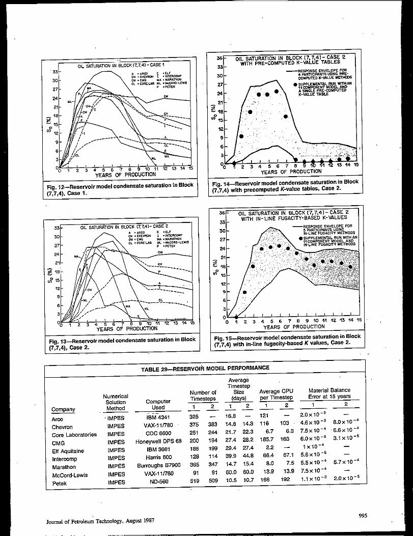
Condemate saturation in Node (7,7,4) is shown in Figs.12 and 13. Most of the models achleye a fiairlystable satu-ration of slightly more than irreducible oil saturation(24%). This indicates a condition of reservoir condensateflow i“ this ar~. Before this time, liquid dropout in thelow-pressure region strips liquid from the gas stream. Tbkcontinues until a sm$iflliquid flow begins and the surfaceyield stabilities. The stabilized yield value depends on themixing of injection gas with reservoir gas around theproducer and the contribution of the depleted area behindthe producer to production.
Lster, during cycling, the condensate around theproducer is partly revaporized, and reservoir oil ceasesto flow. Liquid yield ii partly sustained as some heavy-end fmctiom continue to vaporize and arc pmducd. whatis perhaps surprising is the widely different predictionsfor oil 66turation at advmced depletion levels in themodels, ranging from O to more than 22%. We believetht this c8n be explained by the K values used.
We made two supplcnmtmy rms with COMPf1123forCase 2 to demonstmte the impatance of the K-vahc tcch-
Journalof Petroleum Technology, August 1987
1 O,L sfiT!JRATICNIN BLOCK(7.7.4 - CASE?
33 -
32
27
24 -
2?
18 -g ,5
0m 12
9 -
—
(7,7,4), case 1.
Fig. 13—Reservoir model c&densate saturation in BIOCI(7,7,4), Case 2.
36riicOIL SATURATION IN BLOCK (7, 7,41- CASE 2
33WITH PRE-COMPUTEO K-VALUE TABLES
—F@mwy:,EmE&E&Oj: :&30 COMWTED K-W!LUE MEWXS
27 ● w.P&E#mm~:l&whm#N
24 ● ;* ..ASWLE,RE-COMFWEOK-VALUETABLE,.
21 :;q~ 18. :*::.
no ?5..0.
‘:-YEARS OF PRODUCTION
Fig. 14—Resewoir model condensate saturation in Bloc(T,7,4) with precomputed K-value tables, Case 2.
nique. This compositional simulator permits K values to
be entered as a table or as calculated in line in the normalmanner with an EOS. For the run with K values as ta-bles, we used a single K-value table with a constant-volume depletion of the reservoir gas and assumed Kvalues were independent of composition. The supplemen-tary mm made were identicaJ in all respects except forthe treatment of K values.
Figs. 14 and 15 show condensate saturation for the sup-plemental runs. Fig. 14 shows a clear indication of highevaporation rate of condensate obtained with a K-valuetable. Fig. 14 includes the response envelope of compa-nies (Core Laboratories, Elf Aquitaine, Marathon, andfvfcCord-Lewis) that used precomputed K-value tables.It shows a considerable scatter in predkted condensate,but all show rapid condensate evaporation in the late stagesof cycling.
Fig. 15 shows condensate saturation for the supplemen-tal run with 11 components and in-Iine K vahves with an
EOS. The response envelope for aIl companies who used
similar in-line K values is afao shown. These show some-what better agreement with each other and a slower evapo-ration iti the late stages of gas cycling.
Results for Case 1are qualitatively the same as for Case2. Again, companies using precalculated K values foundwide differences in the amount of condensate formed andits rate of evaporation compiwed with companies that usedEOS methods. Surprisingly, there was no obvious corre-lation between the number of components for thebeptanes-plus fractions and the predicted rates of evapo-ration in Node (7,7,4) for the five companies that usedEOS methods.
‘TMsproblem would benefit ffom PVT data that includesome equilibrium tlash data for fed compositions that ex-ist in fhe enrichment zone near the producer. Unforhmate-ly, these data are unavailable and true evaporation rateis unknown at this time. Data of this kind have been meaa-ured in previous compositional simulation studies 24-26and are needed here to decide which answers are.cofrect.
Reservoir model performance is indicated in Table 29.The nature of IMPES models restricted the timestep sizeto a value generally less than 30 days, especially in thelate stages of cycling as the gas formation factor changes.Machine SF-A differences were not factored into the com-parisons, and only the raw data are given. In-Iine EOSmethods seem to increase rnn times, but maJJyother fac-tors are involved.
Conclusions1. Depletion data and lean-gas swelling data for the
retrograde gas conderiaate are matched well by all com-panies.
2. Inearlyyears ofcycling witbpartial pressure main-tenance, the surface oil rates disagree by about 20%. L]q-uid yield in simple pressure depletion (Fig. 4) does notaccount forthis much error. It suggests rlrat differencesin pressure caused by physical property errors (Z factors)and/or surface-separator molar splh emo:s may also beresponsible.
3. Large discrepancies were observedin incrementaloil obtained by gas-sales deferral (Case 2 vs. Case ‘1);therange was3t08% ofinitial ccmdenaateinplace. Theme-dianvalne was 160 MSTB [25.4X10³ stock-tank m3],or about 4.570 of the initial condensate.
996
4. Thegasused forrecyclinE intbe reservoir modelwas considerably richer inC3~ than the lean gas usedfor the swelling tests. This was unavoidable because notall companies had gas-plant capability in the reservoirsimuiator. Nonetheless, it caats doubt on the usefulnessof the swelling dam fortbe problem.
5. Tbe pressure range for the swelliig data was beyondwhat isneeded forcycling. Several companies chose notto match the high pressure range of the swelling data. This~ybevtild, butwedo nothowhow itaffwtdresul-.
6. There inconsiderable disagreement about conden-satesaPwation intheproducing node, Node(7,7,4). Thisis probably because K values are used aa tables or as cal-cuIated inlinewith an EOS. Theproject does notestab-Iish which method gave better answers in this case, bwthere is more scatter when companies attempt to use K-value tables with no data on which to tune. We were un-able to provide these data for this problem.
AcknowledgmentsWe thank Marathon Oil Co. and Computer ModelfingGroup for penniasion to publish thk paper and for provid-ing the necessasy time and support needed to conduct theproject. We thank the participants for their cooperationand well-written responses to the problem. Last, we areindebted to Core Laboratories Inc. for allowing us to usefhe PVT data essential to this problem.
References1.Odeh, A. S.: “Cornpariso” of .%bniom to a Three-Dimensional
A Three-Phase Coning Smdy,S, JPT (March 1986) 345-53,3. Peng, D.Y. a“d Robinson, D. B.: ‘.A New TwwComtam Equation
of SIX.,, s Ind. ad Ens. Ckn. Fund. (1976) 59-64.4. Lohrew., J., Biay, B.C., and C[arli, C.R.: ..CdculainS Viscosities
of Reservoir F1.ids Fmm Their Compositions,z, JPT (Oct. 1964)1171-76 Trans., AJME, 231.
5. Price, H.S. and Coats, K. H.: “L3ireR Methods in ReservoirSimulation,,, SPEJ (June 1974) 295-308; Trans., AJME, 257.
6. Reid, R. C., Prawnitz, J.M., and Sherwcod, T. K.: 7he Properties
of (he. and Liquids, third editkm, McGraw-Hill Book Co., NewYork Citv (1977) 426.
7. N8hiern, L.X., Fong, D. K., and Aziz, K,: .. CompositionalMcdeli”g With An Equation of State,,+ SPEJ (D... 1981) 21,6S7-98.
S. Nghiem, L. X.: ‘<A New Approach to Q.a.si-Newton Methcds with
Aepfi.ation to compositional Modeling,,, pqer SPE 12242presentedat the 1983 SPE Symposium .“ Reservoir Simulation,San Francisco, Nov. 15-18.
9. Kazend, H,, V.XaJ, C. R., and Shank, O. D.: “A. EfficiemMdticmmponem Nummiwd Simulator,’. SPEI (Oct. 1978) 355-68.
10. Coats, K.H. and Smart, G.T.: ‘. Application of a RegressiomBasedEOS PVT Pm8ram to JAmratoty Data,,, paper SPE 11197 presented ,at the 1982 SPE Annual Technical Conference and Exhibition, NewOrleam. Smt. 26-29.., —.,..—. —..
11. Whit-son, C. H.: ,, Characterizing Hydrocmlxm P1.s Fraction,,,paper EUR 183 presented at the 1980 SPE Europe.” Offshore P-tmlemm Conference, London, Oct. 21-24,
13. Meijerink, J. A.: “A New Stabilized Methcd for Use in IMPES.TYP N.mericd Reservoir Simulators,” paper SPE 5247 presentedal the 1974 SPE Annual Tech”ica3 Conference a“d Exhibitbm.Houston, Oct. 6-9.
14. LitOe, I.E. and Kennedy, H. T,: ‘GA Correlatim of the Viscosityof Hydrocarbon Systems Whh Ress.re, TemFamre mdComposition, ” SPEJ (June 1968) 157-62 Tram., AD.4E, 243.
15. Lee, A. L., Gonzalez, M. H., and E&in, B: E.: c4The Viscosity ofNatural Gas&s,,, JPT(Aug. 1966) 997–100$ Trans., ASME, 237.
16. Wats.m, K, M,, Nelson, E. F., and Murphy, G. B.: “Charactaizxionof Petroleum Fractions,,z Ind. cud Etw. Chem (1935) 27, M6&64.
Joumd of Petroleum Techmlogy, AWSUSf1987
17. Whitson,’ C. H.: “Effect of C,+ F?operdeson Equafion-3f-Statepredictions,,, SPEJ (Dec. 19S4) 685-96,
1S. Haaland, S.: “Characterization of North Sea Crude Oils md Pe-troleum Fractiors, 3, MS fhesis, Norwegian Inst. of Technol., U.ef Tmndheim, Norway.
19. Katz, D.L. and Fire.mahadi, A.: -‘Predcting Phase Behavior ofCondemate/Crude-Oil Systems Using Methane InteractionCwffrcients,’, JPT (Nov. 1978) 1649-5% Trans., ASME, 265.
* 20. Kesl.w, M. G,, Lee, B.I., andSa”dIer,S.1.: “A Third Parameterfor Use j. General Thermodynamic Correlations,,, Ind. and &g.Chem. Fund (1979) 18, 49-34.
21. Keslm, M.G. and he, B.I.: %wove Predictim of Enlhalpy off@CdOIIS.”H@ocarbon Pro.. (March 1976) 153-58.
24. Aura, H. D.: “Nooequilibrium Gas Displacement Calculations,”SPEl (Sept. 1961) 13&3@ Tram., A!-ME, 222.
25. Cook, A.B,, Wa3ker,C.J., and Spencer, G.B.: “Realistic K V?.bImof C,+ Hydrmartwts for calculating Oil Vaporizxion.During OasCyclingat Hish pressures,,+JPT(ldy 196!2)S01- It Trans., AIME,246.
26. Fussell, D,D. and Yarkwrcmgh,L.: “The Effect of Phase Data onLiquid Remveiy Dm-img cycling of a Gas Condensate Reservoir, q,SPEJ (April 1972) 9&102.
S1Metric Conversion Factorsatm x 1.013 250* E+05 = Pabbl X 1.589873 E–01 = m3Btu X 1.055056 E+OO =,k.1
Btu/ft3 X 3.725895 E+O1 = !d/m3ft X 3.048* E-01 = m
t13 X 2.831685 E–02 = m3ft3/lbm x 6.242796 E+OI = dm3/kg