CONSORTIUM The Newsletter of the Consortium for Mathematics and Its Applications CONSORTIUM The Newsletter of the Consortium for Mathematics and Its Applications Special Edition: HiMCM Outstanding Papers Number 86 ISSN 0889-5392 Spring/Summer 2004 Page 2 From the Editor’s Desk: Just Say No (To Filtering) Page 3 Henry’s Notes: Why Does A Truck So Often Get Stuck in Our Underpass? Page 5 Historical Notes: The Universality of Mathematics Part 2: The Distant Scene Page 9 Geometer’s Corner: Getting a Better Angle Page 13 Math Today: One Egg or Two? Statistics Helps Shed Light on Paleontology Pull-Out Section: Genetics and A Mathematically Indefensible Historical Movement HiMCM Outstanding Papers Page 19 Everybody’s Problems: Spread of an Infectious Disease
Transcript
CONSORTIUMThe Newsletter of the Consortium for Mathematics and Its Applications
CONSORTIUMThe Newsletter of the Consortium for Mathematics and Its Applications
Special Edition: HiMCM Outstanding Papers
Number 86 ISSN 0889-5392 Spring/Summer 2004
Page 2 From the Editor’s Desk: Just Say No (To Filtering)Page 3 Henry’s Notes: Why Does A Truck So Often Get Stuck in Our Underpass?
Page 5 Historical Notes: The Universality of Mathematics Part 2: The Distant ScenePage 9 Geometer’s Corner: Getting a Better Angle
Page 13 Math Today: One Egg or Two? Statistics Helps Shed Light on PaleontologyPull-Out Section: Genetics and A Mathematically Indefensible Historical Movement
HiMCM Outstanding PapersPage 19 Everybody’s Problems: Spread of an Infectious Disease
A few weeks ago I read anInternet board posting by a woman whoseaccomplishments include
the creation of an award-winning mathWebsite for children.
She described herself as a very goodmath student who came to hate thesubject while taking calculus in college.After finishing calculus, she decidedshe “would NEVER take another mathcourse.” She added that her son, aneven better math student, developed asimilar attitude while pursuing anengineering major.
About the legendary question, “Whydo we have to learn this?” she wrote, “Ithink we need to take that questionvery, very seriously. The question is asignal that what is going on in ourclassrooms is perceived as irrelevant;and probably pretty dull stuff, too. Ifwe can’t justify it with any reasonsbetter than, ‘you’ll need it for the nextclass’ or ‘... for the test’ or ‘... in caseyou become a grammarian/mathematician/whatever,’ then weneed to seriously rethink what we areteaching and why.”
I took her posting quite seriously; inpart because I work for an organizationwhose goal it is to make experienceslike those of the writer and her sonuncommon. But the posting also struckhome: like the writer, my daughtercame to dislike math while takingcalculus in college, and like thewriter’s son, my son began to dislike itwhile pursuing a technical major.
Many people seem unaware thatmathematics is not taught solelybecause it is useful. If utility were theprimary rationale, textbooks andteacher training programs wouldreflect the fact. There are other reasons.Years ago a mathematics professor toldme, “Other departments use us as acleaver.” By that he meant thatrequiring a course that is abstract andirrelevant is a good way to thin theranks. A student who did well in arelevant algebra course after failingone steeped in abstraction onceobserved, “Most people fail atsomething because they have nointerest in it.”
“A pump, not a filter” is a slogan heardthroughout years of mathematics
education reform. I believe that thefiltering role’s prominence can bemeasured by the extent to whichinstruction is bent on coverage andabstraction at the expense of relevance.In his book The Arithmetic of Life andDeath, George Shaffner describes suchinstruction as having “too muchabstraction, too much symbolism, toomuch complexity, too much rigor, andlessons that are too damned long.”
If we are to reject the role ofeducational hit men (or women), thenwe must strive to engage our students,to make our courses relevant, and tohelp our students deepen theirconceptual understanding ofmathematics. This issue of Consortiumcarries writings of teachers andstudents from classrooms in whichthese goals are being realized.Moreover, at COMAP we are workinghard on several new projects designedto help teachers achieve these goals.We invite our readers to watchConsortium and our Website forannouncements and to get involved. ❏
2 CONSORTIUM
From the Editor’s Desk
1-800-772-6627
TOLL FREE
TOORDER
1-800-772-6627
CONSORTIUMConsortium is a quarterly newsletter of the Consortium for Mathematics and Its
Applications, Inc. (COMAP), but it is also much more. Each issue brings lessons and ideas that demonstrate what COMAP believes is an exciting way to
teach and learn mathematics. The center Pull-Out Section of the issue is aclassroom lesson ready to be photocopied and distributed to your students.
If you are interested in receiving Consortium, call 1-800-772-6627 for information about COMAP membership.
This material is developed by COMAP, Inc. Any findings, conclusions, or recommendations expressed are those of the
authors and do not necessarily reflect the views of COMAP, the cooperatingsocieties, or the editorial board. Submissions should be sent to
Consortium Editor, COMAP, Inc.or to the individual department editors.
(COMAP), Inc., Suite 210, 57 Bedford Street, Lexington, MA 02420.(781) 862-7878.
www.comap.com
Publisher: Solomon GarfunkelEditor: Gary Froelich
Department Editors
Geometer’s Corner: Jonathan ChoateHiMCM Notes: William P. Fox
Historical Notes: Richard L. FrancisEverybody’s Problems: Dot Doyle
Henry Pollak spent 35 years at BellLabs and Bellcore doing or managingmathematical research. He retired in
1986, and has been a visitingprofessor of mathematics education
at Teachers College of ColumbiaUniversity since 1987. This column
will discuss mathematical questions and models which find
their origin in either of his careers orin his everyday life. He can bereached at 40 Edgewood Road,
Summit, NJ 07901-3988.
WHY DOES ATRUCK SO
OFTEN GETSTUCK IN
OURUNDERPASS?
WHY DOES ATRUCK SO
OFTEN GETSTUCK IN
OURUNDERPASS?HENRY POLLAK
It just doesn’t seem reasonable that trucks should have as much troubleas they do.After all, in every case I know, the road leading to theunderpass has a sign indicating the clearance. Furthermore, it is natural
to assume that the driver knows the height of the truck and is capable ofcomparing the two numbers and making an appropriate decision.And yet,the problem kept happening. I haven’t kept any records, but I think theyhave decreased the clearance indicated on the sign at least twice in recentyears.What’s the matter, does the railroad bridge over the highway settle alittle more every few years, or is the highway department just unable tohire anyone who can measure the distance between the pavement andthe bottom of the bridge?
Surprisingly, I think it’s neither of these: I think the trouble is that truckshave gotten longer!
I live in Summit, New Jersey. The nameof the community was not the fancifulinvention of a developer’s ad agency, butactually fits the geography: As a train onwhat used to be called the Delaware,Lackawanna, and Western RR makes itsway west from the New York area, it hasto go up several hundred feet to get here.In the old steam days, there was awatering station at which the enginecould take a drink before continuing toMorristown and points northwest, andthat may have contributed to the namingof the town. The road to which I havebeen referring goes directly down theside of the hill, while the track thatcrosses it changes elevation graduallyalong the edge of the same hill. If wedraw a schematic of the height of theroad, and of the bridge, it looks roughlyas follows:
So as the truck goes down the hill, therecomes a time when the cab and the frontwheels are on the horizontal road surfaceunder the bridge, while part of the van,and the rear wheels, are still on the hill.At this point, the middle of the van,being supported by the front wheels onthe flat surface under the bridge and bythe rear wheels still on the hillside, isfurther off the ground than the front ofthe van, and therefore closer to thebridge. It is indeed conceivable that thetruck may get stuck under the bridge,even though its height is less than theheight of the bridge. Nature has jackedup its rear end.
We need to draw a careful picture andintroduce our notation. To simplify themodel a little bit, without in any wayendangering the reality of the problem,we assume that the junction between theflat road surface under the bridge andthe sloping surface on the hillside is notcurved and smooth as it is in the realworld, but a corner. This changes the
location of the truck for only a smallportion of the roadway, and not where itmakes any difference.
We see from the figure that y, thedangerous variable, is given by
y = H sec ϕ + x tan ϕ.
Because of the length of the truck, thereis another relationship between x and ϕ.We redraw the bottom of the abovefigure, between the road surface and theline joining the bottom of the wheels:
By the Law of Sines in triangle ROF, wesee that
= ,
or
x sin θ = L sin (θ – ϕ).
This equation allows us to think of φasour independent variable. When wesubstitute this for x in the equation for y,we obtain
y = H sec ϕ + L tan ϕ
= H sec ϕ + L tan ϕ
= H sec ϕ + L sin ϕ – L cot θ .
Before proceeding further with theanalysis, let us get an idea how big thiseffect might be.
Suppose that H = 12 feet, L = 40 feet, θ = 6°, and ϕ = 3°. Then y, the clearanceneeded, would be 13.07 feet instead of 12feet! That’s a pretty big effect!
To find the worst possible value of ϕ, andhence x, we should take the aboveexpression for y, differentiate it withrespect to ϕ, and set the derivative equalto 0.
= H sec ϕ tan ϕ + L cos ϕ –
L sin ϕ (2 + tan2 ϕ) cot θ.
When we set this equal to 0, we obtain acubic equation for tan φ, namely
tan3ϕ (L cot θ) + tan ϕ (2L cot θ – H) = L.
Since the angles are small, there is verylittle to be gained by attempting variousforms of analytic trickery on thisequation. If ϕ and θ are both small,
tan ϕ ≈ ϕ, cos θ ≈ 1, sin θ ≈ θ.
We multiply the equation by sin θ, andthe equation becomes
ϕ3L + 2ϕL – ϕθH ≈ Lθ.
To first order, then, the ϕ that maximizesy will be given by ϕ = θ/2. Then
ymax ≈ H + L .
In our example, θ = 6° = π/30 radians,and L = 40 feet. So the error of assumingthe clearance is H is therefore 40π/120feet or about 1.05 feet. This matches theprevious computation quite well.
In this problem, the computationalprocess is perfectly stable. The source ofthe instability was the model itself: If youignore the grade of the road, you mayeasily be off in the needed road clearanceby over a foot! The effect just is not small,and if you ignore it, long trucks willindeed get stuck. ❏
θ4
∂∂
yϕ
sincos
2 ϕϕ
sin cos cos sinsin
θ ϕ θ ϕθ
−
sinsinθ ϕ
θ−( )
sinθL
sin θ ϕ−( )x
4 CONSORTIUM
LR
FO x
θ ϕ–θ ϕ
bridge
road
L
H
y
x
θ ϕ
ϕ
The focus of the
story of
mathematics in
western culture
begins essentially with the
Dawn of History (the
appearance of writing) and
extends through the various
Greek eras, the Dark Ages, the
pre-Renaissance, and beyond.
Such a partitioning of history
raises questions about what
was happening elsewhere in
the world in key time
intervals. What mathematical
achievements are thus
identifiable in non-western
culture beginning with the
Dawn of History and
extending through the time
period of the Renaissance?
Many questions arise as such a vastarea of mathematics is explored. Inwhat manner did the level ofmathematical achievement in bothwestern and eastern cultures correlatewith plateaus of achievement in otherareas of learning? Here the gamut ofdiscussion ranges over technology,architecture, the sciences, andliterature. Unfortunately, time andspace do not permit such an ambitiousundertaking. Only a scattered few canbe considered as the story continues.The first concerns another look at theeastern setting, and then, beyond all ofthis, a brief glance at the mathematicsof the New World.
Some of the earliesttraces of Japanesemathematics,corresponding toproductive timeperiods elsewhere in
the world, are lost to historians. Thereis nevertheless evidence of a stronginfluence by Chinese culture,especially in the sense of application,on the mathematics of Korea andJapan.
One of the more tangible evidences ofthis influence is the abacus, thoughsignificant variations on theremarkable calculating device arenoticeable as one moves from onesetting to another. Considerableinterest was attached to the abacus, inJapan as elsewhere, because of itsfacility in dealing with money, weights,and measures. Thus its practical orapplied features overrode the allied
concerns of the development ofmathematics as an academic discipline.
Japanese geometry, as is the universalcustom, included a range ofapproximations to π. This wasaccompanied by basic formulas relatedto the circle and to certain polygonaltypes.
Little can be asserted with certaintyconcerning the state of Japanesemathematics in antiquity. Movingbeyond the time period of the DarkAges in western culture, a moreintensive mathematical assessmentbecomes possible. Paralleling the EarlyGreek Era, names likewise emerged onthe mathematical scene and thusallowed a more definitive look atachievement (as opposed to broadcollective references).
Among the more notable figures of theearly modern era was themathematician Seki Kowa (1642–1708).Born in the same year as Isaac Newton,Kowa made his primary contributionsin the discipline of algebra. Other areasof interest and research were those ofthe calendar, the solving of higherdegree equations, and the solving ofsystems of equations.
It is in this latter area of achievementthat Seki Kowa’s name is bestremembered. Working independently,his delvings into the solving of systemsof equations led to the remarkablemethod of determinants. Names oftenassociated with this development arethose of Gabriel Cramer (1704–1752)
5CONSORTIUM
Historical Notes
JAPANESEMATHEMATICS
THE UNIVERSALITYOF MATHEMATICS
(Part 2: The Distant Scene)
RICHARD FRANCIS
and Gottfried Wilhelm Leibniz(1646–1716). Yet the discovery ofdeterminants by Kowa likely occurreda full decade before that of the Leibnizdiscovery in 1693. The conventionalrestriction of determinants to solvingsystems of linear equations wasexpanded upon by Kowa so as toinclude extended systems of higherdegree.
A Modern Notational Look at Kowa’s Discovery.
If , then
x = = ,
y = = .
Though some notational and symbolicdifferences must be noted in thecontrasting of western and easternapplications of determinant theory,counterparts are found in Kowa’s workto the various row and columnproperties that are today very familiarto the mathematician. Propertydevelopments were motivated by theotherwise tedious techniques ofdeterminant expansion in the absenceof row and column relationships.Included were key properties such as
“The value of a determinant isunchanged if correspondinglynumbered rows and columns areinterchanged.”
This insightful result led to theconclusion that all theorems relating torows implied an equally valid theoremshould the word “row” be replaced bythe word “column.” Moreover, thevalue of a determinant is zeroprovided any two of its rows (or of itscolumns) are identical. Or, the value of
a determinant is unchanged ifmultiples of a given row (or column)are subtracted from the correspondingelements of another row (or column).
Seki Kowa, by profession a teacher ofmathematics, did not venture muchfarther than the realm of algebra in hisadvancement of Japanese mathematics.However, those whom he taught andinfluenced were indeed to carry onwith his example. As a consequence ofthe work of his students, includingTakebe Kenko, these later steps led intoa careful probing of the limit conceptand the appearance in this Orientalsetting of traces of the calculus. Suchtraces, though meager and notincluding the derivative, correspondedtimewise rather closely with Europeanenthusiasm over the newly formulatedconcepts of differentiation andintegration in the Newton and Leibniztradition.
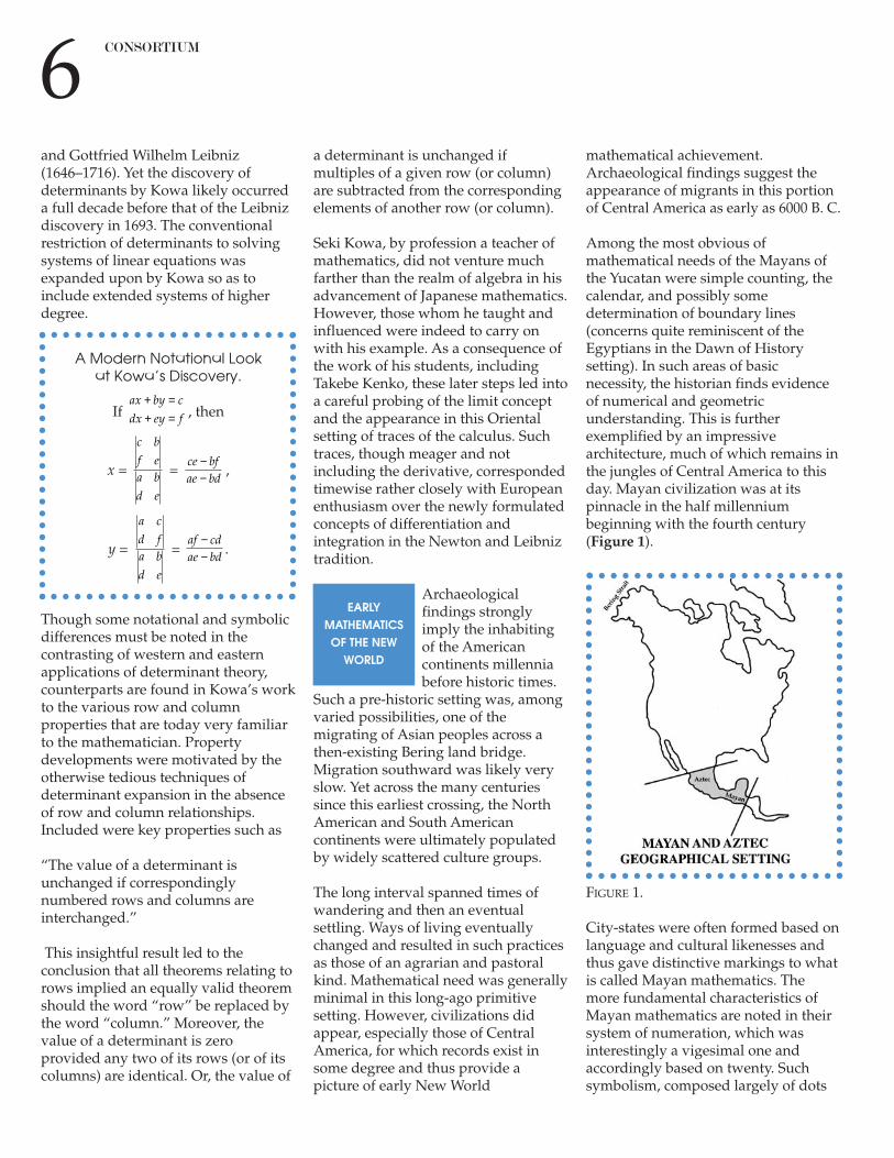
Archaeologicalfindings stronglyimply the inhabitingof the Americancontinents millenniabefore historic times.
Such a pre-historic setting was, amongvaried possibilities, one of themigrating of Asian peoples across athen-existing Bering land bridge.Migration southward was likely veryslow. Yet across the many centuriessince this earliest crossing, the NorthAmerican and South Americancontinents were ultimately populatedby widely scattered culture groups.
The long interval spanned times ofwandering and then an eventualsettling. Ways of living eventuallychanged and resulted in such practicesas those of an agrarian and pastoralkind. Mathematical need was generallyminimal in this long-ago primitivesetting. However, civilizations didappear, especially those of CentralAmerica, for which records exist insome degree and thus provide apicture of early New World
mathematical achievement.Archaeological findings suggest theappearance of migrants in this portionof Central America as early as 6000 B. C.
Among the most obvious ofmathematical needs of the Mayans ofthe Yucatan were simple counting, thecalendar, and possibly somedetermination of boundary lines(concerns quite reminiscent of theEgyptians in the Dawn of Historysetting). In such areas of basicnecessity, the historian finds evidenceof numerical and geometricunderstanding. This is furtherexemplified by an impressivearchitecture, much of which remains inthe jungles of Central America to thisday. Mayan civilization was at itspinnacle in the half millenniumbeginning with the fourth century(Figure 1).
FIGURE 1.
City-states were often formed based onlanguage and cultural likenesses andthus gave distinctive markings to whatis called Mayan mathematics. Themore fundamental characteristics ofMayan mathematics are noted in theirsystem of numeration, which wasinterestingly a vigesimal one andaccordingly based on twenty. Suchsymbolism, composed largely of dots
af cdae bd
−−
a c
d fa b
d e
ce bfae bd
−−
c b
f ea b
d e
ax by c
dx ey f
+ =+ =
6 CONSORTIUM
EARLYMATHEMATICS OF THE NEW
WORLD
and bars, made provision for bothplace value and zero. In spite of theunusual number base, the system wasconducive to the performing of thefour fundamental operations and theextracting of certain roots. Evidenceexists that suggests the actualperforming of these more advancedoperations by the Mayans.
The Mayan calendar, an impressivemathematical achievement, surpassedthose of other New World civilizationsof this early time period. In line withthe vigesimal nature of their system ofnumeration, the year was partitionedinto eighteen months of twenty dayseach and was accompanied by “leapyear” modifications. Its features wereso refined that the prediction of bothsolar and lunar eclipses becamepossible. Their architecture andengineering suggest traces of still moreadvanced mathematical capability. Asthe pre-Columbian era drew to a close,Mayan culture was in some state ofdecay and for many years followingwas given little historicalacknowledgment concerning itstechnology, way of life, andmathematical advancements.
The Aztecs, also of the North Americancontinent, had developed a form ofwriting as well as a system ofnumeration. Their system ofnumeration, based on twenty, likelystemmed from the number of one’sfingers and toes and is thus aninteresting variant on the digitalconcept. Such a system was of arelatively simple nature and wascomposed of varying pictures todenote key number values. Includedwas a scheme for the expression anduse of fractional quantities.Application of these symbols was thatof weights and measures, counting,astronomy, and a relatively accuratecalendar. All of these areas ofapplication gave evidence of theirnumeration system’s vigesimal nature.An intermingling of astronomy andastrology implied a strong religious
influence on Aztec mathematics.However, the numerological overtonesin various calendar cycles do notpreclude a degree of insight, thoughbasic, into certain forms of geometryand trigonometry.
Unfortunately, records of Azteccivilization were destroyed in greatmeasure. It was a loss which resultedin a disturbing gap in the historicalrecord. Aztec culture flourished fromthe beginning of the thirteenth centuryto the times of Spanish conquest byHernando Cortez in the early sixteenthcentury.
The Incan civilization of SouthAmerica, without a written language,did produce a system of numeration(Figure 2). This system, in contrast tothat of the Aztecs and the Mayans, wasbased on ten and allowed for simplecounting and the most elementaryforms of arithmetic. Though areasonably accurate calendar wasdeveloped, it was oriented moretoward agricultural concerns (thecoming and going of the seasons) anddid not reflect a detailed study ofastronomy. Their engineering feats,especially of an architectural andbridge-building nature, suggest a moreadvanced knowledge of mathematicsthan that of numeration and simplecounting. The most thriving timeperiod of Incan civilization extendedfrom the mid-fifteenth century to themid-sixteenth century and encompasseda region of the South Americancontinent ranging from Ecuador in thenorth to Chile in the south.
Early New World culture provides noremnants of what may be regarded asfamous problems in mathematics.However, it does provide a piece in aworldwide puzzle that wouldotherwise be glaringly incomplete. Theuniversal nature of mathematicalinterests and appropriate applicationare suggested, even here, in ageographical setting far removed fromthe mainstream of classical
mathematical activity that hasgenerally been the focus of theconventional historical look.Unfortunately, such a New World pieceof the puzzle, because of themeagerness of records, still leavesunanswered a vast assortment oftantalizing questions.
FIGURE 2.
The intermingling ofmathematical ideasdates from the earliestof time periods.Including commercialcontacts involving
Egypt, Crete, and Greece in the earlyThalassic Age, or the spreading ofGreek culture through the extensivemilitary conquests of Alexander theGreat, mathematical influences wereovertly and subtly involved. Therecord gives abundant evidence ofsuch periods of peaceful and violentinteraction. Still at other times andplaces in history, a high degree ofisolation dominated the scene.
Because of navigational contacts,Greek culture was significantlyinfluenced by earlier civilizations ofnearby lands which bordered on theMediterranean as well as thosesomewhat to the east. Conjectures
7CONSORTIUM
A CULTURALBLENDING OF
IDEAS
concerning discoveries in remotestantiquity of geometric relationshipsand their eventual assimilation into themathematics of neighboring nationshave long fascinated the curious as thehistorical record is examined. Not alldiscoveries have arisen independently,and thus raise the question of howother culture groups happened tobecome knowledgeable of such facts.The story is sometimes obscured byour inability to decipher long-lostlanguages. Many such encounters donot have the same positive outcome asthat of the Rosetta Stone discovery.
As the varied cultures are studied,virtually without fail some form ofnumeration is noted. Thesenumeration systems, vastly different insymbols and scheme, were oftenreplaced by superior systems asawareness of the more sophisticatedsystems filtered through. The story ofthe transmission of Hindu-Arabicnumerals into western culture is one ofthe most significant happenings of thepre-Renaissance.
Some forms of mathematical discoverydo not have this feature of diversefinding or development. As notedbefore, early abstract mathematicsmakes virtually no appearanceanywhere in the world except in theclassical Greek environment. Hence, anappeal to other civilizations andculture groups (as in China or theOrient in general) sheds little light onthe subject of how a form ofdemonstrative geometry is born.
Envision for a moment an alien visitor,looking for the first time at the state ofearthly mathematical achievement.Think too in terms of the advancedmathematical awareness such anobserver might possess. Would it notprove intriguing to witness the alienreaction to an assessment of the manycenturies of worldwide attachment toEuclid’s fifth postulate? This ancient,
wordy pronouncement has auniqueness that arouses curiosity. Onewould accordingly have to wonderhow the notions of the point, the line,the plane, and of space itself, arose inthe alien’s far-off setting. Thusemploying the Greek word for “world”instead of the inappropriate “geo” for“earth,” the question becomes one of“kosomonometry” and its evolution ona distant but enlightened planet. Suchreflections go beyond the bounds ofthe conventional question of theearthly origin and development ofmathematical concepts. Still, thequestion proves insightful in thebroader, more fanciful setting.
Famous problems of varying kinds,affording a meaningful perspective ofhistory, often appear in the sameunique manner of postulationalgeometry. These include, among otherthings, one of the earliest of suchproblem types, namely, the threefamous problems of antiquity. Stillothers, as in the solving of Diophantineequations, suggest variants on thetheorem of Fermat in scattered places.Even as traces of famous problems canoften be found in diverse cultures, thematter of inductive speculation asopposed to rigorous proof must also betaken into account. How might, forexample, an early disposition of the“Pythagorean Theorem” differ as thehistorical scene shifts from Egypt toChina to Greece?
The picture, across the millennia, isparadoxically one of great contrast andsimilarity. However, the later years ofthe modern era are decidedly lessfragmented in this respect. Themathematical community of the earlytwenty-first century is a worldwidecommunity and does not present apicture of the isolation and accidentalintermingling of ideas that sodistinguished the earlier years. ❏
Francis, R. L. 2000. “HistoryCondensed to a Year.” Consortium(74): pages 3-6.
Mikami, Y. 1913 The Development ofMathematics in China and Japan.New York: Chelsea Press.
Morley, Sylvanus G. 1947. The AncientMaya. London: Oxford UniversityPress.
Ordish, George. 1969. The History of theIncas. New York: Random House.
8 CONSORTIUM
Richard L. Francis (ed.) is a professor ofmathematics at Southeast Missouri State
University, where he has taught since 1965. Hismajor scholarly interests include number theory
of the history of mathematics.
Historical Notes concerns insights that focus onthe history of mathematics. The chronological
setting extends from that of a remote timeperiod to the present day. Highlighted in such
accounts are the varied perspectives relating toconcepts, time periods, and mathematicians, be
they well-known or otherwise. Historicalmaterial that lends itself to classroom use so as
to instill mathematical appreciation within the student is especially appropriate.
For more information contact: Richard L.Francis, Department of Mathematics, Southeast
Missouri State University, Cape Girardeau, MO, 63701
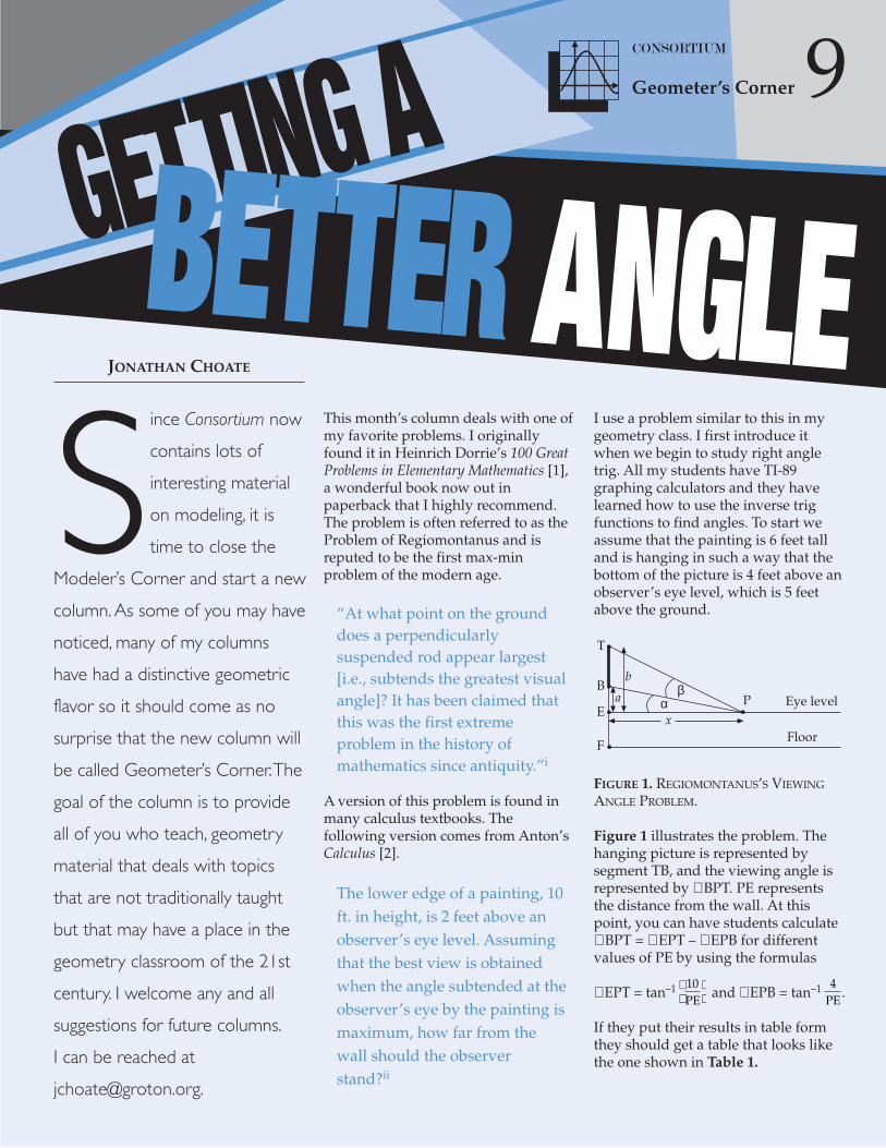
This month’s column deals with one ofmy favorite problems. I originallyfound it in Heinrich Dorrie’s 100 GreatProblems in Elementary Mathematics [1],a wonderful book now out inpaperback that I highly recommend.The problem is often referred to as theProblem of Regiomontanus and isreputed to be the first max-minproblem of the modern age.
“At what point on the grounddoes a perpendicularlysuspended rod appear largest[i.e., subtends the greatest visualangle]? It has been claimed thatthis was the first extremeproblem in the history ofmathematics since antiquity.”i
A version of this problem is found inmany calculus textbooks. Thefollowing version comes from Anton’sCalculus [2].
The lower edge of a painting, 10ft. in height, is 2 feet above anobserver’s eye level. Assumingthat the best view is obtainedwhen the angle subtended at theobserver’s eye by the painting ismaximum, how far from thewall should the observerstand?ii
I use a problem similar to this in mygeometry class. I first introduce itwhen we begin to study right angletrig. All my students have TI-89graphing calculators and they havelearned how to use the inverse trigfunctions to find angles. To start weassume that the painting is 6 feet talland is hanging in such a way that thebottom of the picture is 4 feet above anobserver’s eye level, which is 5 feetabove the ground.
FIGURE 1. REGIOMONTANUS’S VIEWING
ANGLE PROBLEM.
Figure 1 illustrates the problem. Thehanging picture is represented bysegment TB, and the viewing angle isrepresented by ∠ BPT. PE representsthe distance from the wall. At thispoint, you can have students calculate∠ BPT = ∠ EPT – ∠ EPB for differentvalues of PE by using the formulas
∠ EPT = tan–1 and ∠ EPB = tan–1 .
If they put their results in table formthey should get a table that looks likethe one shown in Table 1.
4PE
10PE
9CONSORTIUM
Geometer’s Corner
T
B
E
F
P Eye level
Floor
βαx
b
a
JONATHAN CHOATE
GETTING ABETTER ANGLE
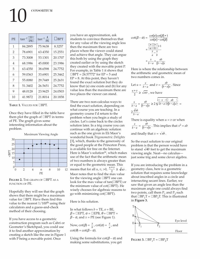
TABLE 1. VALUES FOR ∠ BPT.
Once they have filled in the table havethem plot the graph of ∠ BPT in termsof PE. The graph gives someinteresting information about theproblem.
FIGURE 2. THE GRAPH OF ∠ BPT AS A
FUNCTION OF PE.
Hopefully they will see that the graphshows that there might be a maximumvalue for ∠ BPT. Have them find thisvalue to the nearest 1/100th using theircalculators and a guess-and-checkmethod of their choosing.
If you have access to a geometricconstruction program such as Cabri orGeometer’s Sketchpad, you could useit to find another approximation bycreating a sketch like the one in Figure 1with P being a movable point. Once
you have an approximation, askstudents to convince themselves thatfor any value of the viewing angle lessthen the maximum there are twoplaces where the viewer could standand achieve that angle. They can arguethis both by using the graph theycreated earlier or by using the sketchthey created with the movable point P.For example, in Table 1 it shows that∠ BPT = 24.57772º for EP = 5 and EP = 8. At this point, they haven’tfound the exact solution but they doknow that (a) one exists and (b) for anyvalue less than the maximum there aretwo places the viewer can stand.
There are two non-calculus ways tofind the exact solution, depending onwhat course you are teaching. In ageometry course I’d return to theproblem when you begin a study ofcircles. Let’s come back to the circlessolution later. In a trig course you cancontinue with an algebraic solutionsuch as the one given in Eli Maor’swonderful book Trigonometric Delights[3], which, thanks to the generosity ofthe good people at the Princeton Press,is available for free on the Internet.Here is Maor’s solutioniii, which makesuse of the fact that the arithmetic meanof two numbers is always greater thanor equal to the geometric mean. This means that for all u, v, >0, ≥ .Maor notes that to find the max valuefor the viewing angle ∠ BPT one canlook for the max value of tan(∠ BPT) orthe minimum value of cot(∠ BPT). Hewisely chooses for algebraic reasons togo with minimizing cot(∠ BPT).
Here is his solution.
In what follows b = TE, a = BE, β = ∠ EPT, α = ∠ EPB, θ = ∠ BPT = β – α, and x = PE (see Figure 1).
Now, cot(β) = , cot(α) = , and
cot(θ) = cot(β – α).
Using the formula for cot(β – α) andmaking some substitutions, you get
cot(β – α) =
Here is where the relationship betweenthe arithmetic and geometric mean oftwo numbers comes in.
Let u = and v = . Since
≥ , we have
+ ≥ 2 =
2 .
There is equality when u = v or when
= . This implies that x2 = ab
and finally that x = .
So the exact solution to our originalproblem is that the person would haveto stand feet to get the maximumviewing angle. Neat—no calculus—just some trig and some clever algebra.
If you are introducing the problem in ageometry class, here is a geometricsolution that requires some knowledgeabout inscribed angles in a circle andintersecting secant lines. Earlier, wesaw that given an angle less than themaximum angle one could always findtwo points, call them P1 and P2 suchthat ∠ BP1T = ∠ BP2T. This is illustratedin Figure 3.
FIGURE 3. ∠ BP1T = ∠ BP2T
40
ab
abb a x−( )
xb a−
abb a−
xb a
abb a x−
−( )
abb a x−( )
xb a−
uvu v+
2
abb a x−( )
xb a−
=−
+−( )
xb a
abb a x
=
+
−
xa
xb
xa
xb
1
cot cotcot cot
α βα β
( ) ( ) +( ) − ( )
1
xa
xb
uvu v+
2
10 CONSORTIUM
T
B
EP2
Eye level
Floor
P1
Maximum Viewing Angle
30
<B
PT
PE
25
2015
10
5
00 2 4 6 8 10 12
PE tan–1 tan–1 ∠ BPT
1 84.2895 75.9638 8.3257
2 78.6901 63.4350 15.2551
3 73.3008 53.1301 20.1707
4 68.1986 45.0000 23.1986
5 63.4350 38.6598 24.7752
6 59.0363 33.6901 25.3462
7 55.0080 29.7449 25.2631
8 51.3402 26.5651 24.7752
9 48.0128 23.9625 24.0503
10 41.9872 21.8014 20.1858
4PE
10PE
There is something special aboutpoints B, T, P1 and P2 that will jumpout at you if you think of the segmentBT as being a chord of a circle and∠ BP1T and ∠ BP2T as being inscribedangles in a circle. All four points lie ona circle! If P is the point where themaximum occurs, then the circlethrough B and T will intercept the eyelevel line in only one place and hence itmust be tangent at that point. Now thepicture looks like Figure 4.
FIGURE 4. THE EXACT SOLUTION TO THE
VIEWING ANGLE PROBLEM.
There is a theorem that relates secantlines to tangent lines, which says inthis case that TE · BE = EP2. In ourexample, TE = 10, BE = 4 so EP = ,the same answer we got analytically.
Let’s go a bit farther with the problemand come up with a way to constructthe circle tangent to the eye level lineusing only Euclidian tools. Here is oneway of doing it.
Locate a point Q on line BE such thatQE = BE and Q-E-B.
Construct the midpoint M of segmentTQ.
Construct the circle with center M thatpasses through point T.
Construct a perpendicular to TQthrough E and label its intersectionswith circle M as S1 and S2.
S1 is the desired point of tangency.
Construct the circle C2 through T, Band S1.
Note that ∆QS1T is a right triangle andS1E is the altitude to its hypotenuse.Since the altitude to the hypotenuse isthe geometric mean of the twosegments into which it divides thehypotenuse you can show that S1E2 = QE · TE. S1 is the desired pointof tangency.
FIGURE 5. GEOMETRIC CONSTRUCTION OF
MAXIMUM VIEWING ANGLE.
An interesting variation to the ArtGallery Problem is finding the bestplace to sit in a movie theatre withraked seating. I found the followingversion on the Grand Valley StateUniversity Mathematics DepartmentWebsite located atwww.gvsu.edu/math/calculus/M201/pdf/movie.pdf.
A movie theatre has a screen that ispositioned at 10 feet off the floor and is25 feet high. The first row of seats isplaced 9 feet from the screen and therows are 3 feet apart. The floor of theseating area is inclined at an angle of20 degrees above the horizontal.Suppose your eyes are 4 feet above thefloor and you want to locate a seat thatgives you the maximum viewingangle. How far up the inclined floorshould you locate the seat?iv
In the Figure 6, TB = 25, BG = 10, GA = 9, ∠ DAE = 20° and CA = 4 andline PH is parallel to line AD. Thisproblem has a similar constructivesolution to that of the art gallery. Youneed to find a point P such that the
circle through T, B, and P is tangent toline PH. In order to do this, you needto construct the point H, which iswhere the line that determines youreye level intersects the wall. Once youhave that point located you need tofind the length of HP, the geometricmean of TH and BH. The length ofsegment CP is how far you shouldplace your seat up the raked floor.
Using the law of cosines, you can findan expression for ∠ BPT. Start with acoordinate system with origin at G. Inthis system T = (0, 35), B = (0, 10), andA = (9, 0). Since line AD has slopetan(20°) and goes through the point (9, 0), its equation in point-slope formis y = tan(20°)(x – 9). Line PH is parallelto line AD and is 4 units above it so itsequation is y – 4 = tan(20°)(x – 9).Therefore, any point on line PH hascoordinates (x, tan(20°)x – 9tan(20°) + 4 ).
Expressing BP and TP in terms of xgives you
BP=
TP =
∠ BPT can now be found using the Lawof Cosines.
∠ BPT = cos–1
A maximum value for this function cannow be found using a graphingcalculator with a maximum function orby calculus. Once you have the
BT TPBT PT
2 2 6252+ −
⋅
x x22
35 20 9 20 4+ − ( ) − ( ) +( )( )tan tano o
x x22
10 20 9 20 4+ − ( ) − ( ) +( )( )tan tano o
40
11CONSORTIUM
T
B
EEye level
Floor
P
T
B
E Eye level
FloorQ
M
S1
C2
C1
S2
T
B
G
Eye level
Raked floorH
A E
scre
en
D
M
PC
FIGURE 6. MAXIMUM VIEWING ANGLE IN
A MOVIE THEATRE WITH RAKED SEATING.
coordinates of P, the length AM can befound, and to the nearest hundredth itis 8.25. Another solution using calculuscan be found atwww.gvsu.edu/math/calculus/M201/pdf/movie.pdf. This solution isderived from UMAP Module 729,“Calculus in a Movie Theatre.”
It is interesting that both variations ofRegiomontanus’s problem can besolved exactly by construction. Bothrequire you to do the following:
Given two points A and B and a linethat does not contain A or B and thatdoes not intersect segment AB,construct the circle that passes throughA and B which is tangent to the givenline.
I leave it to the interested reader todevelop a Cabri or Geometer’sSketchpad solution to the movietheatre problem using a constructionsimilar to the one used to find thesolution to the Art Gallery problem.
Regiomontanus’s original problemabout the suspended rod can also besolved using the following construction:
Given two points A and B and a circlewith center C such that A and B areexternal to C; A, B and C are collinearand A-B-C, construct the circle throughA and B that is tangent to circle C.
Here is a construction usingGeometer’s SketchPad. In Figure 7,circle P is tangent to circle C at Q. Q, C,and P are collinear, and CP extendedmeets circle P at R. Since secants ABand QR intersect at C, AC · BC = RC ·QC. AC, BC, and CQ are known. If welet CQ = r and QP = s, then RQ = 2s,and RC = 2s + r. Therefore,
AC · BC = (2s + r)r
= 2sr + r2
and
s =
FIGURE 7. SOLUTION OF REGIOMOTANUS’SORIGINAL PROBLEM.
Here is how to do the constructionshown in Figure 7.
Step 1. Measure AC, BC, and CD = r,the radius of the given circle.
Step 2. Use the SketchPad’s calculator
to calculate s =
Step 3. With C as center dilate point Dby a scale factor of s/r, creating a pointW. Construct segment CW. Note thatCW has length s.
Step 4. With A as center and CW asradius construct circle A. With B ascenter and CW as radius constructcircle B. Label one of the points ofintersection of the two circles P.
Step 5. Construct a circle with P ascenter that contains point A. This is thecircle tangent to circle C.
Step 6. Label the intersection of circle Pwith circle C, Q.
∠ AZB is the maximum angle!
If you would like a challenge, try thefollowing.
Given a circle C and a line l that doesnot intersect C, let A and B be any twopoints on l. Find the point P on circle Csuch that ∠ APB is a maximum.
If you come up with a solution pleasesend it to me and I’ll publish it in thenext Geometer’s Corner. ❏
References
[1] Dorrie, H, 100 Great Problems inElementary Mathematics, Dover,1965, ISBN 486-61348-8
[2] Anton, Bivens, Davis, Calculus, 7th
Edition, Wiley, 2003, ISBN 0-471-38157-8
[3] Maor, Eli, Trigonemteric Delights,Princeton University Press, 2002,ISBN 0691095418
iDorrie, page 369
iiAnton, page 499
iiiMaor, page 46
ivGVSU web site, page 1
AC BC⋅ − rr
2
2
AC BC⋅ − rr
2
2
12 CONSORTIUM
Send solutions to old problems and any newideas to the Geometer's Corner editor:
Jonathan Choate, Groton School, Box 991, Groton, MA 01450.
B
W
R
A
r
D Q
P
C
AB = 12.2771 cmBC = 8.3759 cm
r = 6.2475 cm
= 5.1061 cmAB · BC – r2
2r
= 0.82AB · BC – r2
2r
r
O ne of the goals of paleontologyis to connect what we learnthrough fossil records of extinct
animals’ biology to the biology ofcontemporary animals. A product ofsuch work is the construction ofphylogenetic trees that trace animalmorphology and behavior acrossmany generations and species ofanimals. The detail in which the mostrecent branches in such trees can bearticulated often overwhelms thedetail possible for the oldest branches.In contrast to biologists who enjoyeasy access to large numbers of livingmembers of the species they study,paleontologists are at the mercy ofwhat is originally recorded in the fossilrecord and what remains intact longenough to surface for examination.Therefore, the excitement generated bythe recent finding of just one very wellpreserved nest of a small dinosaur inMontana, Troodon formosus, isunderstandable. Equallyunderstandable is the paleontologists’desire to extract as much informationfrom the nest as possible. As we willsee, despite their rather paltry n valueof 1, their quest led mathematicians toone of the limits of contemporarymathematics.
13CONSORTIUM7 8 9
4 5 6
1 2 3
0 .
÷
x
–
+ Math Today
PAUL KEHLE & TED HODGSON
Troodon, Reptile, and Avian Biology
Although modern day birds andreptiles are very different species, it isquite likely that they share commonancestors. Anyone who has seenJurassic Park probably remembers theclosing scene of a pelican flying acrossthe ocean’s surface, suggesting thatmodern descendants of extinctdinosaurs are alive and doing quitewell. The tracing of contemporaryanimals to their ancient ancestorsmakes use of every bit of evidenceavailable in living and fossilizedsamples.
Modern day birds form and lay theireggs one at a time, with some timepassing (perhaps a day or so) betweenthe laying of successive eggsbelonging to the same clutch. Reptileslay their eggs all at once in a largedepositing of a complete clutch. Avianancestors also laid their eggssequentially, and there is some reasonto suspect that some of these ancestorshad two ovaries functioning in tandemrather than the single ovary found inmodern birds. Animals with twoovaries functioning in tandem will layone pair of eggs at a time followed bya short interval before laying anotherpair. In trying to trace development ofmodern species, traits such as nestingbehavior, egg formation, method ofegg deposition, and number of ovariesplay crucial roles.
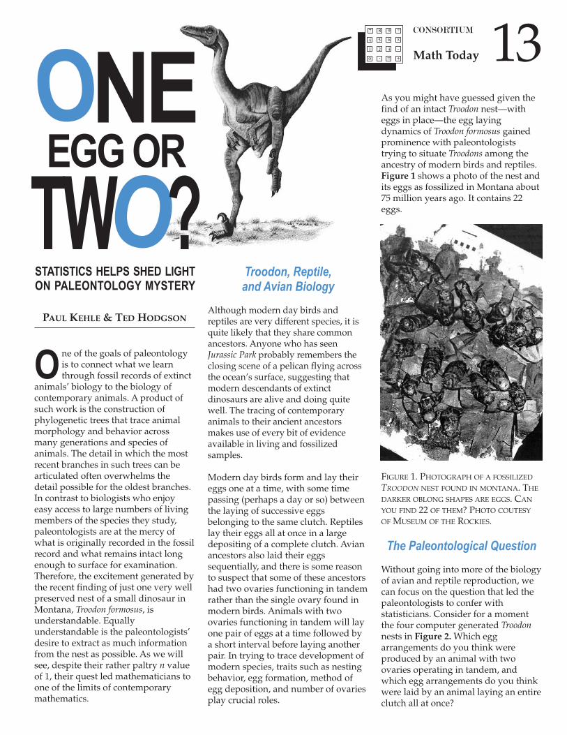
As you might have guessed given thefind of an intact Troodon nest—witheggs in place—the egg layingdynamics of Troodon formosus gainedprominence with paleontologiststrying to situate Troodons among theancestry of modern birds and reptiles.Figure 1 shows a photo of the nest andits eggs as fossilized in Montana about75 million years ago. It contains 22eggs.
FIGURE 1. PHOTOGRAPH OF A FOSSILIZED
TROODON NEST FOUND IN MONTANA. THE
DARKER OBLONG SHAPES ARE EGGS. CAN
YOU FIND 22 OF THEM? PHOTO COUTESY
OF MUSEUM OF THE ROCKIES.
The Paleontological Question
Without going into more of the biologyof avian and reptile reproduction, wecan focus on the question that led thepaleontologists to confer withstatisticians. Consider for a momentthe four computer generated Troodonnests in Figure 2. Which eggarrangements do you think wereproduced by an animal with twoovaries operating in tandem, andwhich egg arrangements do you thinkwere laid by an animal laying an entireclutch all at once?
CONSORTIUM
Unfortunately the fossilized Toodonnest found in Montana was not as clearan example of an egg arrangementproduced by a paired mechanism as isthe simulated nest in the lower leftcorner of Figure 2. When confrontedwith an egg arrangement whose originis uncertain, it is natural to turn tostatistics to assign a degree ofconfidence to the question of whetherthe nest was produced via a paired egglaying mechanism or by a morerandom approach.
It is common for mathematics teachersand students, when posed with theproblem of discriminating betweenpaired and non-paired layingmechanisms, to quickly focus on acomparison of intra-pair distances withinter-pair separations. The intuition isthat if the average of the intra-pair
distances is small compared to theaverage of the inter-pair distances,then a paired mechanism was probablyat work. Similarly, if the average of theintra-pair distances is comparable tothe average of the inter-pair distances,then a paired mechanism was likelynot present.
But this plan is well suited only whenthe likely pairs are easily identified. Insome of the simulated nests in Figure2, we would be hard pressed to pairthe eggs up with any confidence at all.This inability, however, does not meanthat the eggs were not laid in pairs.There is a region of overlap in thepossible distributions of eggarrangements where nests producedby a paired mechanism and nestsproduced by a more random processlook very similar.
In the in-between scenarios, where it isdifficult to decide if a paired orrandom approach was used, we seemin need of a foothold or something touse as a basis of comparison. Thestatisticians provided just such a basis.
The Statistical Answer
We should first state some of theassumptions we are making beforedelving into the mathematical modelused to answer the paleontologists’question. We are assuming that theeggs were not significantly displacedfrom their initial resting spots afterbeing laid, we are assuming that wecan treat the eggs as points in a planerather than paying attention to the fullthree-dimensional aspect of theproblem (in fact the Troodon nest was
14
FIGURE 2.FOUR COMPUTER-GENERATED NESTS AND
EGG ARRANGEMENTS.WHICH WERE GENERATED
BY A PAIRED EGG
MECHANISM, AND WHICH
WERE GENERATED BY A
COMPLETELY RANDOM
MECHANISM?
CONSORTIUM
very flat and no eggs were piled ontop of one another), and when wespeak of a paired versus randommechanism we are not saying thatthere wasn’t a random aspect presentin the paired mechanism. In regard tothis last assumption, the key idea isthat despite the random locations ofthe pairs themselves, the paired nature(the intra-pair distances) wasconstrained by the animal not movingmuch between depositing the twoeggs that belong to a pair.
So, where do we begin to assign a levelof confidence to the hypothesis thatthe Toodon eggs were laid via a pairedmechanism? Although paleontologistsmight be constrained by a very limitednumber of fossilized nests,mathematicians face no suchconstraints. In the abstract world ofmathematics it is often easy togenerate a hundred, a hundredthousand, or a hundred millionsimulated nests. With large numberslike these, we gain statistical powerand confidence not possible whenstudying only one physical nest.
The next key simplifying assumptionmade by the statisticians was tobasically ignore the problem ofmeasuring the inter-pair distances.They sought only to compare theobserved intra-pair distances in thefossil nest with an appropriatestatistical distribution of intra-pairdistances for simulated nests. But thisleft them with the problem of figuringout how to pair up the eggs indistributions where the pairs are notobvious. How could this be done?
The statisticians defined a newmeasurement associated with anydistribution of points in the planecalled the minimum paired distance,or MPD. Consider Figure 3 whichshows all possible pairings of asimulated nest of 6 eggs. The MPD forthis distribution of eggs is theminimum sum (or one of the minimalsums in the event of two or moreequivalent minima) of the intra-pairdistances found across all 15 possiblepairings.
FIGURE 3. ALL 15 POSSIBLE WAYS OF PAIRING A SIMULATED NEST OF 6 EGGS. THE PAIRING
THAT RESULTS IN THE SMALLEST SUM OF INTRA-PAIR DISTANCES IS THE MINIMUM PAIRING
AND ITS ASSOCIATED SUM IS THE MINIMUM PAIRED DISTANCE, OR MPD.
15
16 CONSORTIUM
Given the definition of MPD, we arenow ready to calculate the distributionof MPDs for many simulated nests of22 eggs. In generating these simulatednests, an important issue of scale mustbe addressed. The rough size andshape of Troodon nests, and the degreeto which the eggs are distributedthroughout the interior of the nests,are parameters that have to be setbased on the observed nest. Once theseare determined, the next step is togenerate many simulated nests. Thevital factor in generating these nests isthat the generation be donerandomly—with no pairingmechanism at work. This way we cancompare the MPD for the fossil nestwith the distribution of MPDs for thesimulated nests and determine howsignificantly the fossil nest’s MPDdiffers from the mean of the simulatednests’ mean MPD.
Pause. Remember that when we go towrite a program to generate thesimulated nests and calculate theirMPDs, we will have to first find thepairing of the randomly located 22eggs that yields the MPD, and we willhave to repeat this task for each nest.For 6 eggs there are 15 differentpairings to consider. How manypossible pairings are there for 22 eggs?
Combinatorial Detour
The question of how many pairingsare possible given an even number ofobjects, n, is a nice challenge forstudents studying permutations andcombinations. Both recursive andclosed form expressions are possibleand they seem to be generated equallydepending only on a student’spreferred way of thinking. Theproblem is challenging because afterjust the first couple of cases, thenumber of pairings becomes largequickly. For two objects, there is onlyone possible pairing, and for fourobjects there are three distinct pairings.As Figure 3 shows, there are 15 distinctpairings of six objects, and with theaddition of just two more objects the
number of pairings of eight objectsjumps to 105. Caution: In what followsit will be important to keep straight thedifference between a pair and apairing: Each of the three possiblepairings of four objects has two pairs;similarly, each of the 105 pairings ofeight objects consists of four pairs.
Figure 4 shows how to build the groupof pairings of six objects recursivelyout of the group of pairings of fourobjects. Remember that order within apair or within a pairing doesn’t matter.
If we let Pn represent the number ofpairings of n (where n is any positive
Step 0. Given the three pairings of four objects:
AB CD
AC BD
AD BC
Step 1. Append to each pairing, the new pair EF.
AB CD EF
AC BD EF
AD BC EF
Step 2. Working in turn with each of these three new pairings, sequentiallyexchange one member of each pair with each of the members of the new pairto generate new pairings.
AB CD EF → AE CD BF exchanging B and E
→ AF CD EB exchanging B and F
→ AB CE DF exchanging D and E
→ AB CF ED exchanging D and F
AC BD EF → AE BD CF exchanging C and E
→ AF BD EC exchanging C and F
→ AC BE DF exchanging D and E
→ AC BF ED exchanging D and F
AD BC EF → AE BC DF exchanging D and E
→ AF BC ED exchanging D and F
→ AD BE CF exchanging C and E
→ AD BF EC exchanging C and F
FIGURE 4. GENERATING THE 15 PAIRINGS OF
6 OBJECTS OUT OF THE 3 PAIRINGS OF 4 OBJECTS.
17CONSORTIUM
even integer) objects we can develop arecursive formula for Pn by countingthe numbers of exchanges made foreach of the pairings in Pn – 2. Consider
any n, then there are pairs in
each pairing of the n – 2 objectscomprising the Pn – 2 pairings.
For example, if n = 6, then there are
= 2 pairs in each of the previous
pairings of 6 – 2 = 4 objects. For each ofthese pairs in just one pairing selectedfrom the Pn – 2 pairings, we need tomake two exchanges, once with eachmember of the new pair involved inmoving from Pn – 2 pairings to Pnpairings. So, in step 2 in Figure 4, whenwe were working with the AD BC EFpairing, we had to make twoexchanges in each AD and BCinvolving E and then F. This means we
made 2 · new pairs or simply
n – 2 new pairs. But we also made thevery first new pair based on theprevious AD BC pairing by appending
EF to it. So in all we made 2 · + 1
or (n – 1) new pairs out of just one ofthe previous (n = 4) pairings. We repeatthis process with each of the previouspairings for a total of Pn – 2 times.Hence, Pn = (n – 1) · Pn – 2. Knowingthat P4 = 3, for n = 6, we get P6 = 5 · P4or P6 = 15. Table 1 shows the firstseveral values of Pn.
It is also possible to derive a closedform expression for Pn by consideringfirst all permutations of n objects andthen removing the duplicate pairingsdue to intra-pair ordering and to inter-pair orderings.
Consider n = 6 objects that can bearranged in n! ways in n boxes; andthen consider any one of these pairings(e.g., AE BD CF). See Figure 5.
Each of the pairs within any given
pairing could be in any of two possibleorders (e.g., AE or EA), hence we mustreduce the n! permutations by a factor of 2n/2. Additionally, the pairs
themselves could be in any of !
orders. Applying both of these factorsto n! we get:
Pn =
May I Have the Envelope Please?
Returning to the question of whetherTroodon had one or two ovaries, wewere getting ready to run a computerprogram to generate lots of simulatednests and calculate the MPD for eachnest. We now know that for eachsimulated nest, we will have tocalculate the sum of the intra-pairdistances for each of the 13,749,310,575possible pairings of 22 eggs! If we wantto generate a distribution of MPDs for22 eggs that will allow for a high levelof confidence we will want to look atthousands of simulated nests. Thestatisticians in Montana decided to use 1000 nests in part because of the
time required to compute the needed1.37 x 1013 intra-pair distance sums. Infact, they were able to avoid examiningsome of the pairings least likely to yieldthe MPD, but the problem remainedcomputationally very intensive.
The graphs in Figure 6 show thedevelopment of the increasinglynormal distribution of MPDs forsimulated nests with 6 eggs.
After the statisticians generated their1000 simulated nests of 22 randomlydistributed eggs and then comparedthe MPD of the fossilized nest(requiring another perusal of13,749,310,575 possible pairings) to thisdistribution, they found it was locatedfar to the left of the distribution. Infact, the MPD of the fossilized Troodonnest was smaller than 99% of thesimulated MPDs. On this basis, thepaleontologists concluded with 99%certainty that the Troodon eggs werelaid in pairs lending support to theconjecture that they had two ovarieswhich links them with the ancestors ofmodern day birds.
Remaining MathematicalQuestions and Challenges
In past Math Today columns we’velooked at problems that becomeanalytically and or computationallytoo challenging to solve. In this case,we saw how statisticians were able toanswer a significant question that wasat the border of what iscomputationally feasible. They werefortunate that the fossilized nestcontained only 22 eggs. They mightstill be waiting for their computerprograms to finish running if the
nnn
!
!22
2 ⋅
n2
n2
n2
n −( )22
n −( )22
6 22−( )
n −( )22
A E B D C F
FIGURE 5. DERIVING Pn FROM THE n! PERMUTATIONS OF n OBJECTS WHERE n = 6 BY
TAKING INTO CONSIDERATION DIFFERENCES IN INTRA-PAIR AND INTER-PAIR ORDERINGS
THAT DO NOT CHANGE THE OVERALL NATURE OF ANY ONE PAIRING.
TABLE 1.THE NUMBER
OF DISTINCT
PAIRINGS OF
n OBJECTS.
n Pn
2 1
4 3
6 15
8 105
10 945
12 10395
14 135135
16 2027025
18 334459425
20 654729075
22 13749310575
18 CONSORTIUM
paleontologists had brought them anest of 30 eggs. To find the MPD forjust one nest of 30 eggs would requirelooking at 6,190,283,353,629,375distinct pairings, or 450,225 times asmany pairings as are possible among22 eggs.
Is there a better way? In particular isthere a way to reduce the number ofpairings we must search through tofind the pairing that yields the MPD?Turn your students loose and see whatthey discover. ❏
References
Teppo, A., and Hodgson, T. (2001).Dinosaurs, Dinosaur Eggs, andProbability. Mathematics Teacher,94(2), 86-92.
Tulberg, B. Ah-King, M., & Temrin, H.(2002). Phylogeneticreconstruction of parental-caresystems in the ancestors of birds.Philosophical Transactions of theRoyal Society of London B, 357, pp.251–257.
Varricchio, D. J., Jackson, F.,Borkowski, J., & Horner, J. (1997).Nest and egg clutches of thedinosaur Troodon formosus andthe evolution of avianreproductive traits. Nature, 385:6613, pp. 247–250.
Paul Kehle is a visiting research associate inmathematics education at Indiana University
where he pursues research interests inmathematical cognition and discrete
mathematical modeling. Send results of studentwork on Math Today topics or ideas for future
Sciences, University of the VirginIslands, No. 2 John Brewer’s Bay,
St. Thomas, VI, 00802.
HiMAP Pull-Out Section: Spring/Summer 20042
Mathematical modeling is an important tool in both governmentalpolicy decision-making and in industrial planning. In mathematicalmodeling, we develop a function, a graph, an equation, or asimulation based on assumptions about a situation. The results often
give insight into the situation. The expense of making a mathematical model isusually significantly less than making a prototype. Even more importantly, amath model can sometimes help us avoid making decisions that may havedisastrous effects on humans and our environment.
In this article, we are going to develop and analyze some models related topopulation genetics. In particular, we are going to study how the geneticmakeup of a population changes over time as a result of natural and man-made influences.
We begin by developing models related to the failed “eugenics movement” ofthe late ninteenth and early twentieth century. This worldwide movementpromoted forced sterilization of individuals deemed to have harmful genetictraits. The movement particularly targeted mental retardation, with the goal ofeliminating mental retardation.
Pairs of genes determine many traits, one gene inherited from each parent. The genes come in different forms, called alleles. The particular pair of allelesinherited from the parents determines the trait exhibited by the child. Forsimplicity, we assume there are just two alleles for a certain gene; we willdesignate them A and B.
The possible genotypes are AA, AB, BA, and BB, where the first allele is fromthe mother and the second allele is from the father. We will assume that A is adominant allele and B is recessive, so that the AA, AB, and BA individualsexhibit the trait determined by the A-allele and the BB individuals exhibit thetrait determined by the B-allele.
Let’s assume that the fraction of alleles that are A and B among the parents is pand q, respectively. Since all alleles are of one type or the other, then p + q = 1.We assume that the genetic makeup of males and females are the same, so thatthe probability of a child getting an A-allele from either parent is p.
You Try It #1
Assume that p = 2/3 and q = 1/3. Simulate the births of a population of 36children by rolling a pair of dice 36 times. Mark one die to represent the allelefrom the mother. The other die represents the allele from the father. If thenumbers 1, 2, 3, or 4 come up, then that die corresponds to an A-allele beingreceived from the corresponding parent. If a 5 or 6 shows, then a B-allele isreceived from that parent.
a) What fraction of the children in your simulation have two A-alleles? Whatfraction have one allele of each type? What fraction of the children have twoB-alleles?
b) What fraction of the 72 alleles are A-alleles?
One approach to mathematical modeling is to simulate the situation. YTI#1 is asimulation that gives us some idea of what the genetic makeup of the next
Mathematical modeling can help preventharmful and expensive mistakes.
In 1927, the United States Supreme Courtupheld a Virginia sterilization law, allowingthe forced sterilization of a mentallyretarded woman. It is estimated that by1935, about 20,000 forced sterilizations hadbeen performed in the United States alone.
Sweden, in what is now seen as a nationalscandal, opened the “Swedish Institute forRacial Biology” in the 1920s. During the1940s and 1950s, Sweden sterilized about2000 people per year. Their program wasnot stopped until 1974. (Washington Post,8/29/97)
A child with 2 A-alleles is called a dominanthomozygote. A child with 2 B-alleles iscalled a recessive homozygote. A childwith one allele of each type is called aheterozygote.
generation would look like. Normally, the simulation would generate apopulation larger than 36 to get a better sense of what is happening.
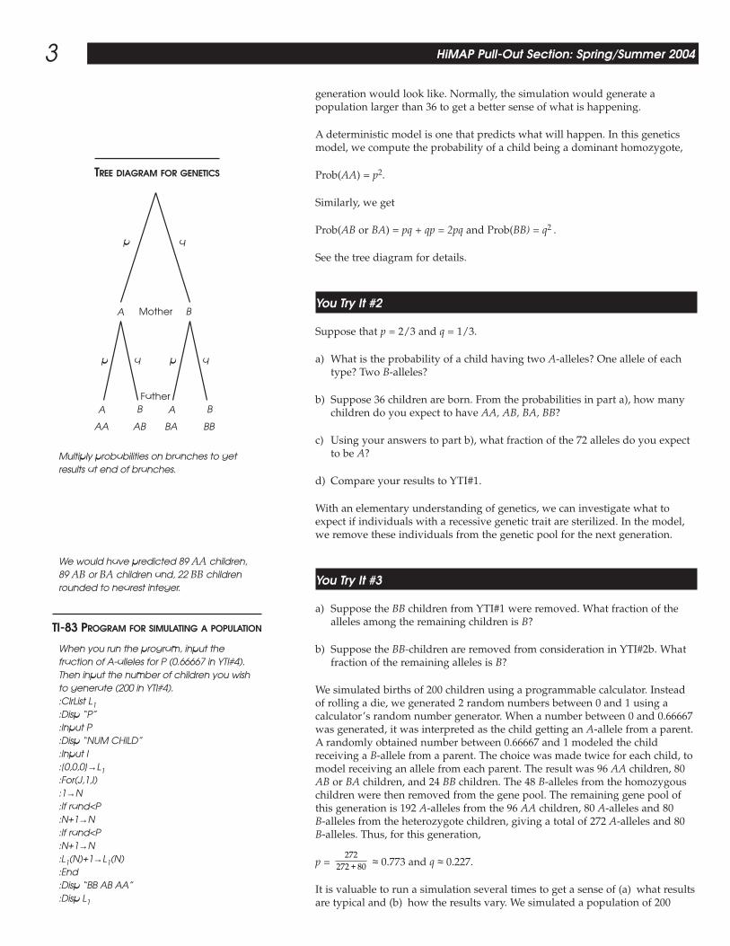
A deterministic model is one that predicts what will happen. In this geneticsmodel, we compute the probability of a child being a dominant homozygote,
Prob(AA) = p2.
Similarly, we get
Prob(AB or BA) = pq + qp = 2pq and Prob(BB) = q2 .
See the tree diagram for details.
You Try It #2
Suppose that p = 2/3 and q = 1/3.
a) What is the probability of a child having two A-alleles? One allele of eachtype? Two B-alleles?
b) Suppose 36 children are born. From the probabilities in part a), how manychildren do you expect to have AA, AB, BA, BB?
c) Using your answers to part b), what fraction of the 72 alleles do you expectto be A?
d) Compare your results to YTI#1.
With an elementary understanding of genetics, we can investigate what toexpect if individuals with a recessive genetic trait are sterilized. In the model,we remove these individuals from the genetic pool for the next generation.
You Try It #3
a) Suppose the BB children from YTI#1 were removed. What fraction of thealleles among the remaining children is B?
b) Suppose the BB-children are removed from consideration in YTI#2b. Whatfraction of the remaining alleles is B?
We simulated births of 200 children using a programmable calculator. Insteadof rolling a die, we generated 2 random numbers between 0 and 1 using acalculator’s random number generator. When a number between 0 and 0.66667was generated, it was interpreted as the child getting an A-allele from a parent.A randomly obtained number between 0.66667 and 1 modeled the childreceiving a B-allele from a parent. The choice was made twice for each child, tomodel receiving an allele from each parent. The result was 96 AA children, 80AB or BA children, and 24 BB children. The 48 B-alleles from the homozygouschildren were then removed from the gene pool. The remaining gene pool ofthis generation is 192 A-alleles from the 96 AA children, 80 A-alleles and 80 B-alleles from the heterozygote children, giving a total of 272 A-alleles and 80B-alleles. Thus, for this generation,
p = ≈ 0.773 and q ≈ 0.227.
It is valuable to run a simulation several times to get a sense of (a) what resultsare typical and (b) how the results vary. We simulated a population of 200
272272 80+
TREE DIAGRAM FOR GENETICS
Multiply probabilities on branches to getresults at end of branches.
We would have predicted 89 AA children,89 AB or BA children and, 22 BB childrenrounded to nearest integer.
TI-83 PROGRAM FOR SIMULATING A POPULATION
When you run the program, input thefraction of A-alleles for P (0.66667 in YTI#4).Then input the number of children you wishto generate (200 in YTI#4).:ClrList L1:Disp “P”:Input P:Disp “NUM CHILD”:Input I:{0,0,0}→L1:For(J,1,I):1→N:If rand<P:N+1→N:If rand<P:N+1→N:L1(N)+1→L1(N):End:Disp “BB AB AA”:Disp L1
HiMAP Pull-Out Section: Spring/Summer 20043
p q
A BMother
p q p q
A BFather
A B
AA AB BA BB
children a total of 10 times and got the following results for q: 0.227, 0.225,0.250, 0.219, 0.236, 0.251, 0.254, 0.250, 0.236, and 0.240. The average of theseresults is 0.24. This is our estimate for the proportion of B-alleles among thechildren’s generation. We now denote q0 ≈ 0.33 and q1 ≈ 0.24 as theapproximations for the genetic makeup of the initial generation and theirchildren.
You Try It #4
a) Simulate the grandchildren’s generation by generating populations of size200 ten times, using p = 0.76. Find the fraction of alleles that are B amongthe AA, AB, and BA children. Approximate q2, the proportion of B-alleles inthe grandchildren’s generation, by averaging your 10 results.
b) Use your result from part a) to generate 10 populations of size 200 amongthe great grandchildren’s generation. Use the result to approximate q3.
You Try It #5
Figure out how our calculator program works.
a) What do the first 5 lines in the program do?
“{0,0,0}→L1“ establishes a list with three items in it, each a zero. The first valuewill tell us the number of BB births (so far), the second value tells us the numberof AB or BA births, and the third value tells us the number of AA births.
“For (J,1,I)…End” is a loop that will run I times. J is the counter and beginswith a value of 1. Each time it reaches the End statement, J increments by 1until it reaches a value of I. Then it goes on to the next statement.
b) What happens inside the loop? First: what does the statement “1→N” do?
c) Second: What does the pair of lines “If rand<P (then) N+1→N” do? (rand isthe random number generator; it produces a number at random between 0and 1.) Why is the pair of lines “If rand<P (then) N+1→N” repeated?
d) In the last line of the loop, L1(N) means the Nth item in our list, L1. Whatdoes the statement “L1(N)+1→L1(N)” do? And, what does it mean in thecontext of our simulation?
e) After the loop runs 200 times (which it will do if we input a value of 200 forI), what will the sum of the numbers in the list L1 be? What will each of theindividual numbers in L1 mean?
In the last 2 lines of the program, we output the results, with labels.
We are now going to predict the fraction of A and B alleles in each generation,assuming that the B-allele is a recessive trait and that all individuals exhibitingthe trait caused by the B-allele are sterilized.
You Try It #6
a) Suppose p0 = 2/3 and there are 200 children born to this generation. Howmany AA, AB or BA, and BB children do you expect? (Be exact; include thefraction.) How many A and B alleles do you expect among the AA, AB, and
It is doubtful in many cases that peoplewho were sterilized as a result of theeugenics movement had a genetic defectcausing mental retardation. In fact, some ofthe people being sterilized may not havebeen mentally retarded.
Suppose a recessive allele causes mentalretardation and that this allele is relativelyrare in the population; that is, B is small. Theresults of our computations indicate that itwill take sterilizing many generations tohave an appreciable affect on theprevalence of B in the population.Remembering that a generation is about 15 years, this indicates that eugenics issomewhat ineffective.
A question that points up another problemwith the eugenics movement is, “Whodetermines what traits are negative?”
HiMAP Pull-Out Section: Spring/Summer 20044
BA children? Use these numbers to predict p1 and q1, given that BB children donot reproduce.
b) Repeat part a) using your calculation for p1 and q1 to predict p2 and q2.
c) Repeat part a) using your calculation for p2 and q2 to predict p3 and q3.
d) Assume that qn = 1/(n + 2). Use this to find pn. Assume there are 200children born to this generation. How many AA, AB or BA, and BB childrendo you expect? How many A and B alleles do you expect among the AA,AB, and BA children? Use these answers to predict qn+1.
e) Suppose that qn = 0.04. How many generations will it take until theproportion of B-alleles is reduced to 0.02?
f) How many generations will it take for the proportion of B-alleles to bereduced from 0.02 to 0.01?
g) How do the predicted results of parts a), b), and c) compare with the resultsof the simulations in YTI#4?
“Common sense” would seem to indicate that sterilizing individuals withharmful traits would reduce the trait in society. But the deterministic modeland the simulations both cast doubt on the effectiveness of eugenics inreducing a “negative” trait from a small fraction of the population to anappreciably smaller one. These genetic models showing the ineffectiveness ofeugenics were not difficult to develop. And yet this movement continuedworldwide for decades.
We now turn our attention to a mathematical model that allows us to estimate avalue that would be difficult to measure directly: mutation rates. We consider asituation in which the recessive trait caused by the B-allele is lethal, where allBB children die before reaching reproductive age. Historically, galactosemiawas such a trait. Modeling this trait is analogous to modeling eugenics, wherethe BB adults were not allowed to reproduce. We add the additionalassumption that a certain percent of the A-alleles mutate to B-alleles, as occurswith the allele for galactosemia.
Let’s assume that p0 = 0.3 and q0 = 0.7 and that 16% of the A-alleles mutate to B-alleles. Using the same program as earlier to simulate a population of 200children, we obtained 25 AA children, 88 AB or BA children, and 87 BBchildren. The genetic makeup of this generation is 50 A-alleles from the 25 AAchildren, 88 A-alleles and 88 B-alleles from the heterozygote children. None ofthe BB children survive. This gives a total of 113 A-alleles and 88 B-alleles.
We now consider the mutation rate. Since 16% of the A-alleles, (0.16)113 ≈ 18,mutate to B-alleles, we then have 113 – 18 = 95 A-alleles and 88 + 18 = 106B-alleles. Thus, for this generation,
p1 = ≈ 0.473 and q1 ≈ 0.527.
You Try It #7
a) Simulate 200 children being born with p0 = 0.3. Find the number of AAchildren and the number of AB or BA children. Use that to get the numberof A-alleles and B-alleles among the children. Subtract 16% of the A-allelesand add that number to the number of B-alleles. Use the totals to estimate p1and q1. Remember that no BB children will live to reproduce.
9595 106+
Galactosemia is a genetic disease thatprevents infants from metabolizing lactoseand galactose. Galactose builds up in theblood, resulting in liver failure. Today,galactosemia is relatively easy to diagnoseand treat.
The prevalence of the recessive allele forgalactosemia is q ≈ 0.006, so p ≈ 0.994. Thismeans that q2 ≈ 0.00036 of children are bornwith galactosemia. This is about 1 in 30,000.
Normal alleles mutate to the allele thatcauses galactosemia.
If a population reaches a point at which itsgenetic makeup remains about the samefrom one generation to the next, then thepopulation is said to be in equilibrium. This iswhat has happened in YTI#7.
HiMAP Pull-Out Section: Spring/Summer 20045
b) Using your estimates for p1 and q1, repeat part a) to get an estimate for p2and q2.
c) Keep using your previous estimates for pn and qn to estimate pn + 1 and qn + 1as you did in part b) until you have estimates for p3 and q3 through p8 and q8.
In YTI#7, you found that the fraction of alleles that are A and B seem tostabilize around positive values instead of one or the other going to 0. Adeterministic model will help us understand what is happening:
You Try It #8
a) Suppose p0 = 0.3 and that 200 children are born. Find the number of AAchildren and the number of AB or BA children expected. Use that to get thenumber of A-alleles and B-alleles among the children. Subtract 16% of the A-alleles and add that number to the number of B-alleles. Use the totals toestimate p1 and q1.
b) Suppose p0 = 0.8 and 200 children are born. Find the number of AA childrenand the number of AB or BA children expected. Use that to get the numberof A-alleles and B-alleles among the children. Subtract 16% of the A-allelesand add that number to the number of B-alleles. Use the totals to estimate p1and q1.
c) Suppose p0 = 0.6 and 200 children are born. Find the number of AA childrenand the number of AB or BA children expected. Use that to get the numberof A-alleles and B-alleles among the children. Subtract 16% of the A-allelesand add that number to the number of B-alleles. Use the totals to estimate p1and q1.
In YTI#8, we saw that there was a value for p and q that remained constantfrom one generation to another. This value is the equilibrium genetic makeupfor the population. We also saw from parts a) and b) that if the genetic makeupis not in equilibrium, then the genetic makeup of the next generation will becloser to the equilibrium value. This shows that over time the genetic makeupof this population stabilizes at equilibrium. Let’s see why this happens.
Suppose 200 children are born to a population where p is the proportion of A-alleles and q = 1 – p is the proportion of B-alleles. Then we expect 200p2 AAchildren and 400p(1 – p) AB and BA children. This gives a total of
Assume that the fraction of A-alleles that mutate to B-alleles is x. Then thenumber of A-alleles remaining after mutation is
400(1 – x)p.
Thus, we have
p1 = = .12
––
xp
400 1400 2
( – )( – )
x pp p
Notice that the proportion of A-allelesincreases.
Notice that the proportion of A-allelesdecreases.
Notice that the proportion of A-allelesremains constant, or is in equilibrium.
In YTI#7 and YTI#8, x = 0.16.
If x = 0.16, this equation becomes
pn =
Check to see if it gives the same answers toYTI#8, parts a, b, and c with pn–1 = 0.3, 0.8,0.6, respectively.
0 842 1
.– –pn
HiMAP Pull-Out Section: Spring/Summer 20046
If x is known, then the equation
pn =
can be used to approximate pn over time. Furthermore, at equilibrium pn = pn–1 = p, so we solve the equation
p =
to find that the equilibrium proportion of A-alleles is
p = 1 ± .
Since q = 1 – p, if p = 1 – then q = . This means that the fraction ofchildren born with BB is q2 = x. Thus, the fraction of children with the diseasecaused by the B-allele equals the mutation rate.
xx
x
12
––
xp
12 1
–– –
xpn
We have discovered that the mutation ratefor galactosemia is about 0.000036 or aboutone allele in 30,000.
HiMAP Pull-Out Section: Spring/Summer 20047
You will probably get about 16 AA children, 16 BA or ABchildren, and 4 BB.
About 2/3.
Prob(AA) = 4/9, Prob(AB or BA) = 4/9, and Prob(BB) = 1/9.
Predicts 16 are AA, 16 are AB or BA, and 4 are BB.
2/3
It is likely that the results will be similar, but not thesame.
About
You should get q2 ≈ 0.20 = 1/5.
q3 ≈ 0.17 ≈ 1/6.
Clear List L1 of any values it may have had fromprevious work. Ask for and receive input for a value toassign to P, the probability of an A-allele. Ask for andreceive input for a value of I, the number of child birthsin the simulation you are going to do.
“1→N” makes N = 1.
This command chooses a random number and tests tosee if it is less than the value of P. If it is less, this isinterpreted as receiving an A- allele from the first parent.The command is repeated to determine whether an A-allele is received from the second parent.
“L1(N)+1→L1(N)” adds 1 to one of the elements of thelist. If both random numbers were > P (of which there isprobability 1 – P), we interpret this as the birth of a BBchild. In this case, the value of N will not change; N willstill be 1. So the statement causes “L1(1)+1→L1(1); that is,the first item in the list increases by 1. This means wehave added 1 to the number of BB births. If one of therandom number choices is < P and the other is > P, weinterpret this as an AB or BA birth and increase the valueof N by 1; L1(2)+1→L1(2). Finally, if both randomnumber choices are less than P, the “child” is AA, so thethird number in the list increases by 1.
The sum L1(1)+L1(2)+L1(3) will be 200, or whatevernumber you input for I, the number of births you wantto simulate. The list started at 0, 0, 0, and one of theentries increased by 1 each time the program wentthrough the loop. It looped I times, so if we input 200 asthe value of I, the sum of the outcomes will be 200. Theindividual entries give the number of BB births, thenumber of BA or AB births, and the number of AAbirths, in that order.
88 AA children, 88 AB or BA children, and 22
BB children. This gives 266 A-alleles and 88 B-alleles.
q1 = = 1/4 so p1 = 3/4.
112.5 AA children, 75 AB or BA children, and 12.5 BBchildren. This gives 300 A-alleles and 75 B-alleles. q2 = = 1/5 = 0.2 so p2 = 4/5 = 0.8.
128 AA children, 64 AB or BA children, and 8 BBchildren. This gives 320 A-alleles and 64 B-alleles. q3 = = 1/6 ≈ 0.167 so p3 = 5/6 ≈ 0.833.
pn = . There will be 200 AA children,
400 AB or BA children and 200 BB children.
This gives 400 B-alleles and 400
A-alleles. The number of B-alleles divided by the total
number of alleles simplifies to qn + 1 = =
= .
If qn = 0.04 = 1/25, then n = 23. We want qm = 1/50, so m = 48. This is an additional 25 generations. If ageneration is about 20 years, this is 500 years.
If qn = 0.02 = 1/50 then n = 48. We want qm = 1/100, so m = 98. This is an additional 50 generations (another1000 years).
Results should be reasonably close.
p1 ≈ 0.5 and q1 ≈ 0.5.
p2 ≈ 0.56 and q2 ≈ 0.44.
The results for pj approach 0.6; qj approaches 0.4.
18 AA children and 84 AB and BA children giving 120 A-alleles and 84 B-alleles. 19.2 A-alleles mutate to B-alleles giving 100.8 A-alleles and 103.2 B-alleles. Thus,p1 = 100.8/204 ≈ 0.494 and q1 ≈ 0.506.
128 AA children and 64 AB and BA children giving 320A-alleles and 64 B-alleles. 51.2 A-alleles mutate to B-alleles giving 268.8 A-alleles and 115.2 B-alleles. Thus,p1 = 268.8/384 = 0.7 and q1 = 0.3.
72 AA children and 96 AB and BA children giving 240 A-alleles and 96 B-alleles. 38.4 A-alleles mutate to B-alleles giving 201.6 A-alleles and 134.4 B-alleles. Thus,p1 = 201.6/336 = 0.6 and q1 = 0.4.
13n +
nn n
++( ) +( )
11 3
nn n
++ +
14 32
n nn
2
2
3 22
+ ++( )
nn
++( )
12 2
12 2n +( )
nn
++( )
12 2
nn
++
12
2nn
++
12
64384
75375
8889
35559
89
23
29
89
89
14
14
Answers to You Try Its HiMAP Pull-Out Section: Spring/Summer 2004
6
b
b
b
b
b
c
d
e
c
d
2 a
3 a
4 a
5 a
1 a a
7 a
8 a
b
c
b
c
b
c
d
e
f
g
8
Partial funding provided by IBM
Additional support provided by the National Council of Teachers of Mathematics (NCTM),
the Mathematical Association of America (MAA),
and the Institute for Operations Research and Management Sciences (INFORMS).
H I G H S C H O O L M AT H E M AT I C A L C O N T E S T I N M O D E L I N G
O U T S TA N D I N G PA P E R S
Editor’s CommentsThis is our sixth HiMCM Special Issue. Since space does not permitprinting all of the nine national outstanding papers, this special sectionincludes the summaries from six of the papers and edited versions ofthree. We emphasize that the selection of these two does not imply thatthey are superior to the other outstanding papers. They were chosenbecause they are representative and fairly short. They have receivedlight editing, primarily for brevity. We also wish to emphasize that thepapers were not written with publication in mind; the contest does notallow time to revise and polish. Given the 36-hour time limit, it isremarkable how well written many of the papers are.
November
We appreciate the outstanding work of students andadvisors and the efforts of our contest director andjudges. Their dedication and commitment have madeHiMCM a big success. We also wish to note that thisspecial section takes the place of our regular HiMCMNotes column, which will return in the next issue.
The contest offersstudents the
opportunity tocompete in a team setting
using applied mathematics
in the solving of real-world
problems.
2003
Contest Director’s ArticleWilliam P. Fox
Department of MathematicsFrancis Marion UniversityFlorence, SC [email protected]
The High School Mathematical Contest in Modeling (HiMCM)completed its sixth year in excellent fashion. The growth ofstudents, faculty advisors, and the contest judges is very evidentin the professional submissions and work being done. The contestis still moving ahead, growing in a positive first derivative, andconsistent with our positive experiences from previous HiMCMcontests.
This year the contest consisted of 275 teams (a growth of about30% from last year) from twenty-five states and from outside theUSA. This year was the first year that schools were charged aregistration fee of $45 for the first team and $25 for eachadditional team.
Thus our contest continues to attract an international audience.The teams accomplished the vision of our founders by providingunique and creative mathematical solutions to complex, open-ended,real-world problems. This year the students had a choice of twoproblems. Of the 275 teams, 156 submitted solutions to the Bproblem, and 119 submitted solutions to the A problem.
Problem A: What is it Worth?In 1945, Noah Sentz died in a car accident and his estate was
handled by the local courts. The state law stated that 1/3 of allassets and property go to the wife and 2/3 of all assets go to thechildren. There were four children. Over the next four years, threeof the four children sold their shares of the assets back to themother for a sum of $1300 each. The original total assets weremainly 75.43 acres of land. This week, the fourth child has suedthe estate for his rightful inheritance from the original probateruling. The judge has ruled in favor of the fourth son and hasdetermined that he is rightfully due monetary compensation. Thejudge has picked your group as the jury to determine the amountof compensation.
Use the principles of mathematical modeling to build a modelthat enables you to determine the compensation. Additionally,prepare a short one-page summary letter to the court that explains your results. Assume the date is November 10, 2003.
Problem B: How Fair are Major LeagueBaseball Parks to Players?Consider the following major league baseball parks: AtlantaBraves, Colorado Rockies, New York Yankees, California Angles,Minnesota Twins, and Florida Marlins.
Each field is in a different location and has different dimensions.Are all these parks “fair”? Determine how fair or unfair is eachpark. Determine the optimal baseball “setting” for major leaguebaseball.
COMMENDATION:
All students and their advisors are congratulated for their variedand creative mathematical efforts. The thirty-six continuous hoursto work on the problem provided (in our opinion) a vastimprovement in the quality of the papers. Teams are commendedfor the overall quality of work.
Again this year, many of the teams had female participation,which shows that this competition is for both male and femalestudents. Teams again proved to the judges that they had “fun”with their chosen problems, demonstrating research initiative andcreativity in their solutions.
JUDGING:
We ran three regional sites in December 2003. Each site judgedpapers for both problems A and B. The papers judged at eachregional site were not from their respective region. Papers werejudged as Outstanding, Meritorious, Honorable Mention, andSuccessful Participant. All regional finalist papers for the RegionalOutstanding award were brought to the National Judging. Forexample, eight papers may be discussed at a Regional Final andonly four selected as Regional Outstanding but all eight papersare brought and judged for the National Outstanding. Thenational judging chooses the “best of the best” as NationalOutstanding. The National Judges commend the regional judgesfor their efforts and found the results were very consistent. Wefeel that this regional structure provides a good prototype for thefuture of the contest’s structure as it continues to grow.
JUDGING RESULTS:
National & Regional Combined Results
GENERAL JUDGING COMMENTS:
The judges’ commentaries provide comments on the solutions toeach of the two problems. As contest director and head judge forthe problems, I would like to speak generally about teamsolutions from a judge’s point of view. Papers need to be verycoherent, concise, and clear. Students need to restate the problemin their own words so that the judges can determine the focus ofthe paper. Papers that explain the development of the model,
HiMCM OUTSTANDING PAPERS2
Outfield Dimensions Wall Height
Franchise Left Left Ctr Right Right Left Ctr Right Area ofField Ctr Field Ctr Field Field Field Field Fair Ter
Angels 330 376 408 361 330 8 8 18 110,000
Braves 335 380 401 390 330 8 8 8 115,000
Rockies 347 390 415 375 350 8 8 14 117,000
Yankees 318 399 408 385 314 8 7 10 113,000
Twins 343 385 408 367 327 13 13 23 111,000
Marlins 330 385 404 385 345 8 8 8 115,000
Problem National Regional Meritorious Honorable Successful TotalOutstanding* Outstanding Mention Participant
A 4 12 33 45 25 119
B 5 10 42 75 23 155
Total 9 14 51 104 33 274
assumptions, and its solutions and then support the solutionfindings mathematically generally do quite well. Modelingassumptions need to be listed and justified but only those thatcome to bear on the team’s solution (that can be part ofsimplifying the model). Laundry lists of assumptions that arenever referred to in the context of the model development are notconsidered relevant and deter from the paper’s quality. The modelneeds to be clearly developed, and all variables that are used needto be defined. Thinking outside of the “box” is also an ingredientconsidered important by judges. This varies from problem toproblem but usually includes model extensions or sensitivityanalysis of the solution to the teams’ inputs. A clear conclusionand answers to specific scenario questions are all key components.The strengths and weakness section of the paper is where theteam can reflect on the solution. Attention to detail andproofreading the paper prior to final submission are alsoimportant because the judges look for clarity and style.
CONTEST FACTS:
Facts from the 6th Annual Contest:
• A wide range of schools/teams competed including teams fromHong Kong.
• The 275 teams represented 60 institutions; 44 repeats and 16new institutions.
• 44.36% of the teams had female participation. Forty-three of the275 teams were all female.
• There were 953 student participants, 548 male (57.5%) and 395female (42.5%).
• Schools from 25 states participated in this year’s contest.
THE FUTURE:
This HiMCM contest that attempts to give the underrepresentedan opportunity to compete and achieve success in mathematicsendeavors appears well on its way in meeting this important goal.
We continue to strive to grow. Any school/team can enter thecontest, as there will be no restrictions on the number of schoolsentering. A regional judging structure will be established based onthe response of teams to compete in the contest.
Again, these are exciting times for our high school students.Mathematics continues to be more than learning skills andoperations. Mathematics is a language that involves our dailylives. Applying the mathematical principles that one learns is keyto future success. The ability to recognize problems, to formulate amathematical model and solve it, to use technology, and tocommunicate and reflect on one’s work is key to success. Studentsdevelop confidence by tackling ill-defined problems and workingtogether to generate a solution. Applying mathematics is a teamsport.
Advisors need only be a motivator and facilitator. They shouldpermit students to be creative and imaginative. It is not thetechnique that is fundamental, but the process that discovers howassumptions drive the techniques. Mathematical modeling is an
art and a science. Through modeling, students learn to thinkcritically; communicate efficiently; and be confident, competentproblem solvers for the new century.
Contest Dates: Mark your calendars early: the next HiMCM willbe held in November 2004. Registrations of teams are due inOctober 2004. Teams will have a consecutive 36-hour block withina window of about two weeks to complete their chosen problem.Teams can registrar via the worldwide web at www.comap.com.
HiMCM Judges Commentary
Problem A: What is it Worth?Although some teams initially believed that this was a simplealgebraic problem involving the time value on money (i.e., aFuture Value = P(1 + I)R problem), it soon became apparent to thebetter teams that they needed to perform some modeling andcritical analysis of the situation.
The judges were impressed with the creativity, quality of theanalysis, and the writing by the teams modeling Problem A.Teams dealt with time value of money, and they dealt with thevalue of land over time. It was imperative for teams working withland value to assume or “pick” a location (county or state) inorder to estimate through modeling the appreciation of the land’svalue. Doing this provided teams an opportunity to restate theproblem in more manageable terms. This allowed successfulteams to move from the general ill-defined problem to anattackable, more specific, defined problem.
Many teams attacked this problem only as a time value of moneyissue. A key aspect here was obtaining an interest rate or indexgrowth rate over time. Research as to which values were the mostappropriate was necessary. Many teams merely stated values. Judgesexpected the teams to develop a sub-model to determine this.
One of the items that distinguished the better papers was thatthose teams calculated the “worth” from various models (money,land, etc.) and then came to a final conclusion aboutcompensation after considering all their possible outcomes.
Verification of models or model testing was also an importantdiscriminator. Some teams tested their models to see if the resultsmade common sense. Others compared their predictions withhistorical results that they were able to obtain via web sources. It isnoted that some answers given by teams made little practical sense.
Problem B: How Fair are Major LeagueBaseball Parks to Players? This was the purest modeling problem of the two. This problemwas ill defined because students needed to determine what theymeant by “fair.” Teams needed to step back and insure that theyhad a well-defined problem, defined “fair,” and determinedwhich aspects of “fair” they were trying to model.
Some teams did not define “fair” until after they completed theirmodels, which was deemed too late by many judges.
HiMCM OUTSTANDING PAPERS 3
The judges commented that the statement of assumptions withjustification, style of presentation, and depth of analysis was verygood. The better papers offered a good diversity of solutions.Problem B, in comparison to Problem A, appeared to lend itselfbetter to consideration of a variety of assumptions andjustifications.
It was critical for teams to define “fair” in order to compare thebaseball parks. The judges were surprised that no teamrecommended changing the dimensions of ballparks in order tomake them more “fair” based on their mathematical findings. Thebetter papers considered such variables as altitude, wind,humidity, temperature, and other environmental factors in theirmodel or their discussions of the model.
Many papers used computer code to determine the issue offairness of the baseball parks. Computer codes used to implementmathematical expressions can be a good modeling tool. However,judges expect to see an algorithm or flow chart in the paper fromwhich the code was developed. Successful teams provided someexplanation or guide to their algorithm(s)—a step-by-stepprocedure for the judges to follow. The code that teams attachedto their paper may only be read for those papers that reach thefinal rounds of judging. The results of any simulation or computercode need to be explained, and sensitivity analysis should beperformed.
For example, consider an algorithm for the flip of a fair coin:
An algorithm such as this would be expected in the body of thepaper with the code as an appendix.
The judges commend the teams for a truly outstanding job on adifficult, open-ended problem that provided some interestingreading.
GENERAL COMMENTS FROM JUDGES:
Executive Summaries:
These are still, for the most part, one of weakest parts of teamsubmissions. These should be complete in ideas not details. Theyshould include the “bottom-line” and the key ideas used. Theyshould include the particular questions addressed and theiranswers. Teams should consider a three paragraph approach:restate the problems in their own words, give a short descriptionof their method to model and solve the problem (without givingspecific mathematical expressions), and state the conclusions,including the numerical answers in context.
Restatement of the Problem:
Problem restatements are important for teams to move from thegeneral case to the specific case. They allow teams to refine manyaspects of their thinking to give their model uniqueness and acreative touch.
Assumptions/Justifications:
Teams should list only those assumptions that are vital to thebuilding and simplifying of their model. Assumptions should not bea reiteration of facts given in the problem description. Assumptionsare variables (issues) acting or not acting on the problem. Everyassumption should have a justification with it. Variables chosenneed to be listed with notation and be well defined.
Model:
Teams need to show a clear link between the assumptions theylisted and the building of their model or models.
Model Testing:
Model testing is not the same as testing arithmetic. Teams need tocompare results or attempt to verify (even with common sense)their results.
Teams that use simulation must provide a clear step-by-stepalgorithm for the proposed simulation. Lots of runs and relatedanalysis are required when using a simulation to model aproblem. Sensitivity analysis is also expected to determine howsensitive the simulation is to the model’s key parameters.
Conclusions:
This section deals with more than just results. Conclusions mightalso include speculations, extensions to the model, andgeneralizations of the model. Teams should ask themselves whatother questions would be interesting if they had more time andthen tell the judges about their ideas.
Strengths and Weaknesses:
Teams should be open and honest here. They should answer thequestion, “What could we have done better?”
HiMCM OUTSTANDING PAPERS4
INPUT: Random number, number of trials
OUTPUT: Heads or tails
Step 1: Initialize all counters.
Step 2: Generate a random number between 0 and 1.
Step 3: Choose an interval for heads, like [0.0.5]. If therandom number falls in this interval, the flip is a heads. Otherwise the flip is a tails.
Step 4: Record the result as a heads or a tails.
Step 5: Count the number of trials and increment: Count = Count + 1.
References:
Teams may use references to assist in modeling the problem.However, they must also identify the sources. It is still requiredof the team to show how the model was built and why it wasthe model chosen for this problem. Teams are reminded thatonly inanimate resources may be used. Teams cannot call uponreal estate agents, bankers, or any other real person to obtainany information related to the problem.
Adherence to Rules:
Teams are reminded that detailed rules and regulations areposted on the high school contests area of the COMAP Website.Teams are reminded that the 36-hour time limit is a consecutive36 hours.
Problem A Summary:Clarkstown South High SchoolAdvisor: Mary Gavioli
Team Members: Simi Bhat, Daniel Gendler, Mitchell Livingston, Terry Van Hise
When the rightful inheritance of a beneficiary is not givenshortly after the probate court’s original ruling, finding anappropriate amount of compensation for that inheritance iscomplicated by several factors. Noah Sentz’s fourth childshould have been awarded 1/4 of 2/3 of his estate according tostate law at the time of Mr. Sentz’s passing. However, the fourthchild is now suing for compensation because he did not receivehis portion of the estate. There were several factors weconsidered when calculating Mr. Sentz’s compensation, themost important of which being inflation. Inflation is theprogression of changing value of a dollar over time. This meansthat the items a dollar could purchase when Mr. Sentz passedaway probably would not cover the price of that item at thepresent time. We found the inflation rate from the time that thethree children sold their portions of the estate to the present tobe 802.9%. This means that if the land was worth $1200 andother personal assets were valued at $100 then, then the landwould be worth $9624 and the other personal assets wouldhave a value of $802.90 now. We also took into account therevenue the fourth child would have been deprived of becausehe did not own the land since 1945. The total amount ofrevenue generated from the land would have been $53,568.However, the fourth son would have had to pay additionalincome tax on this revenue, which would amount to $13,894.80.He would have also had to pay property tax on this land for thepast fifty-eight years, a total of $316.04. To find the finalmonetary compensation the son should be given we summedthe values of all assets and income and subtracted all taxesgiving Nick a final compensation of $49,784.06. We made ageneralized model, allowing for the input of several variablessuch as state and federal income tax rate, original value of land,original value of personal assets, and such variables. To increasethe ease of use of our model, we created a computer program inJava so that court officials could simply input the variables intothe program and receive an output of the calculated monetarycompensation the disputing beneficiary should receive. Themath model we created uses data taken from governmentreferences and economic journals. We feel it is a feasible andaccurate model.
Problem A Summary: Mills E. Godwin High SchoolAdvisor: Ann Sebrell
Team Members: Derek Austin, Srini Sathyanarayanan, Matthew Walker, Zhiyuan Xu
We the jury have determined that the plaintiff, the fourth childof the late Noah Sentz, deserves monetary compensation forassets not awarded in the amount of $18,772.35. Throughinvestigating the problem, we researched various aspects ofinheritance laws as well as the economic factors influencing theasset price. Our amount of compensation is the modem value ofhis portion of the assets minus property taxes accrued since1945. We found this amount of compensation through amathematical model that we created.
We initially created a simple model in which the plaintiff wouldreceive value only from land assets and built upon this. Weestablished the property as rural farmland from Pennsylvania.We realized that rural farmland is highly influenced by inflationand the appreciation of land value. By tracking basic land valuepatterns, we were able to roughly estimate the value of land in2003. Through researching Consumer Price Index weapproximated the influence of the cost of living on the price ofconsumer goods, which we then included in the model as partof his compensation. We decided that the four children initiallysplit the consumer goods while the mother received her portionof the estate only in farmland; in other words, we accounted foran uneven split in the type of assets distributed, even thoughthe amount of assets for each group was even. Finally, wededucted a 9.5% property tax rate from the estimated value ofthe land portion of his share of assets to create a final amount ofcompensation.
Through thorough examination of various factors influencingthe value of the estate, we can confidently conclude that thecompensation for the fourth child’s inheritance in this situationshould be $18,772.35.
Problem B Summary: Maggie L. Walker Governor’s SchoolAdvisor: John Barnes
Team Members: Guilherme Cavalcanti, Thomas Fortuna, Mrinal Menon, Derek Miller
Our first step in evaluating whether or not the fields were fairwas to hypothesize that teams with a greater penchant forhitting home runs would build smaller stadiums to hit morehome runs, while teams that could not hit as many home runswould build larger stadiums in order to deprive other teams ofhome runs. We then gathered available team data for three tofive years before each team built their current stadium, trying todetermine if their home run performance in relation to theirleague affected the creation of their fields. No relationship wasfound between team performance and the pure dimensions ofthe field as far as home runs were concerned.
We then decided to test if the initial velocity of a baseball hit ateach field was significantly different in a perfect, airless world.It was determined that there was no significant difference in
HiMCM OUTSTANDING PAPERS 5
initial velocity for each stadium. Research, however, revealed thatthere was a significant difference in the amount of home runs hitat each of the six assigned stadiums, specifically Coors Field. Theonly construction difference between Coors Field and all otherstadiums was its extreme altitude. We then proceeded to modifyour baseball projectile motion model to include air resistance, toaccount for changes in altitude and temperature. Two forms ofEuler’s method were used to model the trajectory of a baseballthrough a dense atmosphere. This updated model revealed thataltitude and temperature were major factors in determining afield’s fairness; hitting home runs at sea level fields required amuch greater initial velocity.
We then proceeded to define fairness in our fields. Our first beliefwas that fields that are symmetrical about their centerlines (rightand left field distance and wall heights are equal) are fair to bothright-handed and left-handed hitters. Of the six stadiums, ProPlayer Stadium of the Florida Marlins was the only one that couldbe considered fair. The remaining five teams in increasing fairnessare the Denver Rockies, New York Yankees, Atlanta Braves, andAnaheim Angels. The Twins’ stadium, being temperaturecontrolled, did not apply to our model. We also believe that we cancreate a fair field distance by taking average distances of existingfields that are getting league average home runs, accounting fortemperature and altitude variations. Using these two beliefs andour air resistance model, we can create a “fair” field knowing onlythe altitude, temperature, and uniform wall height.
Problem B Summary: Illinois Mathematics and Science AcademyAdvisor: Steven Condie
Team Members: Jeffrey Chang, Alex Garivaltis, David Xu
To begin tackling the problem, we decided to use a nationalbatting average of 0.25 as an indicator of fairness. Our vision ofthe “fairest” field was one that provided its players with a level ofoffensive and defensive opportunities consistent with the nationalaverage. Therefore, a ballpark that produced a batting averageclosest to the national average was considered to be the optimalsetting. The model consisted of a computer program that wouldautomatically calculate the players’ positions on a Cartesian planegiven the dimensions of a field. To determine the batting averagefor any of the given ballparks, we created an algorithm thatwould simulate 10,000 at-bats, taking into account appropriateratios for strikeouts and foul-outs. The variables Θ (initial anglewith respect to ground), v0 (initial velocity of the ball), and Φ(angle of ball’s direction of travel on Cartesian plane) were allrandomized within reasonable ranges for each simulation.
The program then analyzed the trajectory of the ball, taking intoaccount the wind speed and any effects from low air pressure. Bycalculating the position of the ball’s landing spot, our modeldetermined whether the ball would be caught (resulting in anout), would not be caught (resulting in a safe base advance), orwould fly over the fence as a home run (counting as four baseadvances). Our simulation was able to compute the battingaverage by keeping track of the number of base advances over10,000 simulations.
To assess the fairness of the stadiums played in by the Angels,Braves, Rockies, Yankees, Twins, and Marlins; we found the
batting averages resulting from each ballpark’s specificdimensions and environmental conditions. The resulting order offairness for the ballparks, from fairest to least fair, was:
To determine the optimal setting in general we decided to employan evolution-based simulation method. The program generated arandom set of field dimensions within reasonable limits andcalculated the expected batting average using 10,000 at-batsimulations. The computer then continued generating randomballparks, calculating the batting average every time. Whenever aballpark resulted in a batting average that was closer to thenational average than any previously checked ballpark, it becamethe new optimal setting. After repeating this process for a longtime, the best setting naturally surfaced.
Problem B Summary: Dubuque Hempstead High SchoolAdvisor: Karen Weires
Team Members: Tom Duggan, Josh Lichti, Cory McDermott, Brad Willenbring
To quantitatively compare the fairness of the given stadiums, wedefined numerous variables and methods of measurement. Acomputer program was created to simulate the behavior of hits ineach stadium, taking into account its dimensions and prevailingenvironmental conditions. The program also simulated thedistance the outfielders need to move in order to field all non-homerun hits. This data was coupled with numerous other factorsincluding backstop length and field orientation to determine eachstadium’s Defensive Bias Rating (DBR), a measure of howoffensively or defensively biased the given ballpark is.
The DBR value was then factored into the calculation of anothervalue, the Oppositional Equality Rating (OER), a measure of howwell matched a given team is to their stadium. A team that hitswell overall, stationed in a stadium that caters to a hitting team, isgoing to have a distinct advantage because they play 50% of theirgames on their home field.
The DBR and OER both proved to be very accurate models ofreal-life conditions among the stadiums in question. The Coloradostadium was determined to be the most unfair stadium based onits OER rating. Environmental conditions make hits in Coloradotend to fly further, coupled with a team that statistically (already)seems to prefer offense to defense. In other cases, such as Atlanta,the team’s ability wasn’t paired with its stadium, so the twocanceled each other out in the OER rating.
HiMCM OUTSTANDING PAPERS6
Outfield Dimensions Wall Height
Left Left Ctr Right Right Left Ctr RightField Ctr Field Ctr Field Field Field Field
Problem B Summary: Mills E. Godwin High SchoolAdvisor: Ann Sebrell
Team Members: Deepa Iyer, Brandon Murrill, Omari Stephens, David Williamson
During our investigation of this situation, our team aimed toderive an optimal model for fairness in a baseball park. To achievethis goal, we created a list of ten factors that we felt could affectthe fairness equilibrium of a field. We researched thespecifications of these ten factors and found an abundance of datafrom various sources.
By analyzing the magnitude of the effect of each factor at all of thesix parks, we created a score for each park that led us to ourconclusions. We found that each park was biased toward theoffense or the defense; none was completely fair.
We tested our models by comparing the classifications wegenerated to the historical conception of each park: whether thevenue was considered more favorable for a hitter or a pitcher.
We then proceeded to develop an optimal, completely fair baseballenvironment. We strove to ensure that our park favored neither theoffensive or defensive team. Finally, we generated two strategies todevelop a fair stadium. The first method required different factorsto favor either the offense or the defense; the total effect of all thefactors remained at equilibrium. The second method called fornearly neutral values for every single factor, again yielding aneutral venue overall. We combined the two strategies to developa realistic, optimal design for a truly fair field.
Problem A Paper: The Spence SchoolAdvisor: Eric Zahler
Team Members: Jillian Bunting, Madeleine Douglas, Yi Zhou
PROBLEM RESTATEMENT
Noah Sentz died in a car accident in 1945. His wife received one-third of his estate, and the children received two-thirds. Over thenext four years, three of the four children sold their shares back totheir mother for $1300 each. Noah’s assets were mostly comprisedof 75.43 acres of land. In early November 2003, the fourth childsued for his rightful share. The judge ruled that he is due cashcompensation.
LETTER TO THE COURT
We created a mathematical model for determining the plaintiff’scompensation. We made several assumptions to produce aneffective model. These included the dates of the death of NoahSentz and the subsequent sale of his assets by his three sons, thatthe first son received only land, that the value per acre wasuniform, that the non-land assets appreciated at the rate ofinflation, and that the values of each child’s share was equal in 1945.
Besides these, our model made no assumptions about the specificvalues of variables. Instead, all variables are available to bemanipulated. This is a very effective way of determining
compensation because it can be implemented in a variety ofsituations. This is especially important because certain factors (i.e., value per acre, appreciation of land) are specific togeographic regions.
The benefits of our model are that it gives a fairly good range ofvalues for the compensation and that it leaves only one factor tobe determined by the court (the value of land per acre in 1945).Even without determining the value per acre, our model tells usthat the compensation due the fourth son is between $55,400.39and $90,162.43. Our model is also strong because it made noarbitrary assumptions. The inflation rates between years werebased on historical data. The land appreciation rate was inferredfrom national data.
We feel confident that our inflation and land appreciation ratesare fairly accurate. Therefore, we respectfully recommend that themodel be used to determine compensation after the price per acreis determined.
ASSUMPTIONS AND JUSTIFICATIONS
In 1945, the worth of each child’s share was equitable. We assumethis because none of the children sued within four years. The suitdid not arise until 58 years later, implying that there was noproblem for a long time.
The fourth son received non-land assets that did not appreciate asfast as the land. He is suing for the difference between what hisshare is worth now and one-sixth of what the estate would beworth today.
Mr. Sentz died in January of 1945. We assumed this in order tohave a base date to calculate inflation.
The first, second, and third children sold their shares back to theirmother in January 1947, January 1948, and January 1949,respectively. This allowed us to find inflation values. We chosedates spread evenly over the four-year period to reflect thechanging inflations over those four years.
The value of the land per acre is uniform. This allowed us torelate our equations to one another, and simplifies the problem byeliminating a variable.
All other assets appreciate at the rate of inflation. This simplifiesthe problem.
The rate of land appreciation is constant and reflects the best-fitcurve that we found (see Figure 1 and Appendix B). This allowedus to create equations; with land appreciation as a variable, thereis too much unknown. We considered it reasonable to assume thatthe land appreciation was roughly equal to the overall trend in theUnited States.
The first son only received land. We assumed this in order tosimplify the problem and allow us to solve for the value of theland in 1945.
HiMCM OUTSTANDING PAPERS 7
OUR APPROACH
Land appreciates faster than the rate of inflation (see Appendix Afor a proof). Since other assets appreciate at the rate of inflation,their growth over a long period of time is less than that of land.As a result of a discrepancy in distributing land and other assets(the fourth child only received non-land assets), the fourth child’sshare has not appreciated at the same rate as the land. Thus, if wecalculated how much a sixth of the entire estate would be worthnow and how much the fourth child actually has, the differencewould be how much the fourth child is entitled to.
VARIABLES
L, with subscripts corresponding to children and mother, is theamount of land in acres each received. A subscript of M refers tothe mother, a subscript of 1 refers to the first child, a subscript of 2refers to the second child, and so forth. V is the value per acre in1945. A is the rate of appreciation of land per year since 1945. S,with subscripts corresponding to the subscripts of L, is the valueof the non-land assets the children received in 1945. T is the totalvalue of the estate in 1945. I is the inflation rate between 1945 andthe given year. P is the total value of non-land assets in 1945.Finally, t is the number of years since 1945. From these variables,we generated these equations:
P = S2 + S3 + S4 + SM. The total value of the non-land assets isequal to the sum of what was distributed.
T = 75.43V + P. The total value of the estate is the sum of the valueof the land and the value of the other assets.
V(L1 + L2 + L3 + LM) = 75.43V. The sum of all land distributed isequal to the total value of the land.
L1V = L2V + S2 = L3V + S3 = S4 = (LMV + SM)/2. This comes fromthe assumption that at the time of distribution, each child receiveda sixth of the estate, and the mother received a third.
At t years from January 1945, the value of person X’s inheritancecan be expressed: (LXV)(1 + A)t + (SX)(1 + I1945M).
The trend in a graph of national trends in land appreciation(Figure 1) appeared exponential. We ignored the dip at the end ofthe graph because the trend of exponential growth continues, asevidenced by Figure 2. We estimated coordinates on the land-value graph in Figure 1. From these we found an exponentialmodel (see Appendix B). The general form of the exponentialmodel was y = abx, where a is the starting value and b is theincrease per year. We determined b was 1.0857. Thus landappreciates at a rate of 8.57% per year. Our calculated a was 100.Using this equation, we calculated the value of each child’s sharebased on the value of the first brother’s share, which was entirelyland.
1 + A = b = 1.0857
(L1V)(l + A)2 = 1300
(L1V)(l.0857)2 = 1300
(L1V) = $1102.87, which is the value of each child’s share in 1945.
To determine the value of the estate in 1945, we multiplied 1102.87by 6 and obtained $6617.21 = T. We looked up the inflation ratebetween January 1945 and November 2003: 940.45% (seeBibliography). So the fourth brother’s share is now worth:
November 2003 Value = 1102.87(1 + I2003)
$11474.81 = 1102.87(10.4045).
We were told that the estate was comprised mainly of land, whichwe took to mean that the land’s value was more than 50% of thetotal estate value, but less than or equal to five-sixths of it, sincethe fourth brother received only non-land assets comprising one-sixth of the total. Thus, we created a range of compensation. If theland is half the total value, then its 1945 value is $6617.21/2 =$3308.605. Then the current value of the entire estate is:
His portion would be a sixth of that, or $70700.13. Then he shouldreceive the difference between that figure and $11474.81:$59225.32. The value per acre would be: 75.43V = 3308.605, or$43.86.
On the other hand, if land constituted everything but his portion,5/6 of the total estate, the value of the whole is:
Then his portion should be $110183.65, which means he shouldreceive $98708.84. The value per acre is: 75.43V = 5514.34, or$71.11 (see Figure 3). The range of compensation is then between$59225.32 and $98708.84. It should be closer to the higher value, as “mainly” seems to imply closer to five-sixths than to half.
The function that determines the compensation is (see AppendixC):
General: – S4(1 + I2003)
Specific: f(V) =
– 1102.87(10.4045).
STRENGTHS OF MODEL
1. The general model needs few assumptions because most of itscomponents are variables. It is flexible in that if only a fewvalues of variables are known, by manipulating the equations asolution can be determined. In this case, only land appreciationand rate of inflation, both of which were found online, werenecessary to find a compensation range. Finding the best valuein that range requires only the value of the land per acre.
2. The general model accounts for assets and property, as well asthe percentage of the total each comprises.
3. The model is easy to use and is not caught up in accounting forthousands of possibilities that arise from ambiguity of thevariables. To account for every possible range of values of eachvariable would spawn a convoluted model that may not yieldan accurate answer.
4. The data needed to use the model are readily available.
1 0857 75 43 10 4045 6617 21 75 436
58. ( . ) . ( . . )V V+ −
( ) ( . ) ( )( . )1 75 43 1 75 436
2003+ + + −A V I T Vt
HiMCM OUTSTANDING PAPERS8
5. The model is fairly comprehensive because it accounts forvarious factors, including land appreciation and inflation rate.
6. The model does not require a jury to use high-level math.Plugging in values and adding to get a total requires only sixth-grade skills.
WEAKNESSES OF THE MODEL
1. The assumption that the value of land was uniform wasnecessary for the general method. A difference in the valuewould make the problem more complicated, as it is nearlyimpossible to account for disparities without knowing otherfactors such as location.
2. The assumption that the assets appreciate at the inflation rate isunrealistic.
3. The assumption that the land appreciation trend is perfectlyexponential ignores other factors that affect it, such as naturaldisasters and location. Also, the land appreciation was derivedfrom one graph.
4. The assumptions of the date of Noah’s death and the dateswhen the brothers sold their shares affect the rate of inflationand land appreciation. This would alter the total calculatedvalue of the estate in 1945.
5. The assumptions that the first brother only inherited land andthat he was the first to sell his shares are crucial. While thelatter assumption is logical (the brother with the most land hadto have sold his shares first or else his land would haveappreciated and not have been worth the same as the assets ofthe other brothers), the former assumption was for convenienceand affects the estate value in 1945.
6. The assumption that the inequity arose because of unequal landdistribution is the basis for the entire model. However, it is notexplicitly stated that such is the case.
APPENDIX A: PROOF THAT THE RATE OF LAND APPRECIATION IS GREATER THAN THAT OF INFLATION
Advanced Real Estate Analysis: Lecture 3. University of Chicago.http://gsbreal.com/urban/Lecture%20Notes.htm
Figure 1. Land Appreciation Trend 1945–1993
Figure 2. Total Annual Returns on Land 1985–1999
Problem B Paper: Evanston Township High SchoolAdvisor: Peter DeCraene
Team Members: Erica Cherry, Chris LeBailly, Eli Morris-Heft, Jean Rudnicki
OUR PARAMETERS FOR FAIRNESS
1. Left-handed batters should gain no advantage over right-handed batters. To ensure this, our field is symmetric about aline through home plate and second base.
2. Given a ball speed (VBALL) and angle of elevation (ϕ), a ballshould be a home run no matter the angle (θ) with respect tothe foul lines at which it is hit.
3. The field should comply with major league rules and traditions,one of which is that the distance from home plate to thecenterfield fence should be more than the correspondingdistances down the foul lines. To adhere to this and complywith parameter 2, the fence is lowered in the middle such that aball that would barely clear the right-field (or left-field) fencewould, counting for distance, barely clear the centerfield fence.The fence is smoothly lowered from right field to center andthen smoothly raised from center to left accordingly.
4. The current average number of home runs is about two pergame. We aim to keep this figure static.
5. We recognize that, even as we strive to achieve parameter 1,there is no way to resolve the fact that a left-handed batter getsa one-step advance towards first base. We believe that the timeit takes to step across home plate is negligible, so thisdiscrepancy is not corrected.
6. We want the amount of fair territory to be consistent with theinformation given in the problem.
PROCEDURE
We constructed a computer simulation that picked a batter ofrandom handedness, threw a random pitch, hit the ball at arandom velocity and angle, and determined whether it was ahome run. With each simulation of a game, we found the numberof home runs. Through research, we found that the number of hitsper game is about 20, and we worked with the dimensions of ourpark until, in accordance with fairness parameter 4, about twohome runs were scored per game. We also ranked in fairness theparks given in the problem.
Our simulation variables are summarized in Table 1 and Figures1 and 2.
The parameter bounds were chosen based on our research. 10% ofthe general population is left-handed; we were unable to find thestatistic for baseball players. The fastball is the pitch from whichthe most home runs are hit and is also the straightest pitch andthe one that flies farthest when hit. The range of θ is derivednaturally from the park’s shape.
PROCEDURE
We researched equations to describe the flight of a hit baseballbased on the speed of the pitch, the speed of the bat, and theinitial angle of elevation, taking air friction into account. Our first
HiMCM OUTSTANDING PAPERS10
Figure 3. Compensation Range
equation shows how much kinetic energy is transferred to theball:
KEBALL = (KEPITCH + KEBAT) (1)
Only a third of the energy is transferred—the rest goes tovibration of the bat and to friction. Replacing KE with
MV2, we have:
MBALLVBALL2 + (2)
VBALL2 = (3)
VBALL = (4)
Thus we have an equation for the velocity of a hit ball.
Since we are designing the park for the real world, we have toconsider air friction. Taking to be the velocity vector of the ball
(note that VBALL is a scalar) and as the drag vector, we have:
= –D (5)
We have a negative on the right side because is contrary to the
motion of the ball. Breaking into component vectors, we get:
= = (6)
Totaling the sum of the forces acting on the ball:
= –D = and = –mg – D = (7)
= and = –g – (8)
D is a constant dependent on air density (ρ), the ball’s silhouettesurface area (A), and the drag coefficient (C):
D = (9)
We researched ρ for each city in which we were given and forEvanston, where we located our ideal park. The silhouette surfacearea is easily determined because major league regulations state that the ball “shall…measure not less than nine nor more than 9
inches in circumference.” Taking the circumference as 9 inches,
A is ≈ 6.626 in2. We modeled C on a graph in The Physics of
Baseball. We tried many regression curves and found that the bestfit was the cubic:
C(VBALL) = (–7.773173 x 10⁻⁵)VBALL3 + 0.013016 x VBALL
2 –0.726969 x VBALL + 0.999441 (10)
In order to derive a function for the position of the ball at time t,we split the forces acting on the ball into x- and y-components. To
5329256π
18
14
ρCA2
Dm
v vy( )ayDm
v vx( )ax
mayv vy( )Fy∑maxv vx( )Fx∑
− ( ) − ( )D v v D v vx y,f fx y,f
f
f
v v( )f
f
v
13
2 2VMM
VPITCHBAT
BALLBAT+
13
2 2VMM
VPITCHBAT
BALLBAT+
13
12
12
2 2M V M VBALL PITCH BAT BAT+
12
12
13
HiMCM OUTSTANDING PAPERS 11
Handedness of Batter 90% right; 10 % left
Velocity of Pitch (VPITCH) 90 ± 5 mph
Velocity of Bat (VBAT) 71 ± 2 mph
Initial Angle of Elevation of Hit Ball (ϕ) 35° ± 5°
Angle of Hit Ball with respect to line A (θ) –45° to 45°
Table 1. Simulation variablesFigure 1.
Figure 2.
derive the x-portion of the ball’s position, we started with theequation:
Fx = max (11)
We also know that:
Fx = –kvx2 = max = m (12)
because the only force acting on the ball in the x-direction is airfriction. We are using k to represent the drag coefficient (about0.0007). Using symbol manipulation, we find:
dvx = dt (13)
Integrating both sides, we get:
dvx = dt (14)
– = t (15)
A little more manipulation gives us:
vx(t) = (16)
This gives us the velocity of the ball in the x-direction at time t.We also want the position at time t, which we derive byintegrating:
px(t) = = dt = (17)
In the y-direction, equations must take into account both airfriction and gravity. We can start the same way as with the x-direction:
Fy = g – kvy2 = may = m (18)
We can make this into a first-order differential equation bydividing m from the second and fourth terms in equation (18):
= (19)
Using equation (19), we formed a slope field and used the initialcondition vy = 52.45 sin(35°) to plot a solution to the differentialequation. We took points from this curve and did a polynomialregression:
If we combine equations (17) and (21), we can find equations forthe position and velocity of the ball at time t:
=
(22)
=
(23)
We used a computer simulation to calculate the position of theball. The simulation uses a fourth-order Runge-Kutta method.Using the changing acceleration and velocity vectors, it calculateseach position of the ball based on the previous. As this methodonly works with first-order differential equations, the accelerationvector presents a problem. We resolved the problem bysubstituting in such a way that the acceleration vector’s second-order equation became a system of first-order equations.
By using equation (8) to find the acceleration in both the x- and y-directions, it was possible to use Runge-Kutta to solve thesystem. Each time the Runge-Kutta algorithm was called, itmoved the baseball forward one time step. Since there was achange in velocity in this step, it was necessary to recalculate thedrag coefficient according to equation (10). In this simulation, thetime step was 0.05 seconds. The Runge-Kutta algorithm wasiterated until y-displacement was negative, meaning the ball hadhit the ground.
When the Runge-Kutta method is called, the position and velocityvectors are stored in a matrix. We wanted to find the ball’s heightat a given horizontal displacement. To do this, the programsearched the matrix and interpolated between the point with x-displacement just greater than what we wanted and the pointwith x-displacement just less than what we wanted.
This algorithm was very useful for figuring out if a hit was ahome run. If we knew how far the ball had to travel to reach thewall, we used the previous algorithm to find the horizontaldisplacement. If the vertical distance was greater than the heightof the wall, then the hit was a home run.
The next task was to find the distance from home plate to thewall. We knew the distance from home plate to left field, leftcenterfield, centerfield, right centerfield, and right field. Since wedid not know what function modeled the shape of the wall, weassumed that it was linear. We broke it up into even sections, eachwith a range of 18° (Figure 3).
Determining the value of θ depended on the batter’s handedness.Right-handers tend to hit the ball towards left center, and left-handers tend to hit it towards right center. A Gaussiandistribution was created to randomly pick the direction the ballwas hit. For right-handers, the mean was θ = 22.5° (leftcenterfield) and for left-handers, the mean was θ = –22.5° (rightcenterfield). For both of these distributions, the standard deviationwas set to 5°. A random number generator picked valuesaccording to the normal curve. These values were then altered tofit the appropriate distribution.
To find the initial speed of a hit ball, we had to know the speed atwhich it was pitched and how fast the batter swung. From these,we used equation (4) to determine the speed of the ball off the bat.We knew that the average fastball is thrown at about 90 miles perhour. From the Gaussian distribution (with a mean of 90 and astandard deviation of 5), we randomly selected the speed of the
km
tv
x x x xx
+
− + − − +−
15 471729 0 032844 0 432209 7 650204 52 326
0
1
4 3 2, . . . . .
v v t v tx y( ) ( ),
mk
kv t m t t t t txln , . . . . .04 5 4 3 21 094346 10 0 008211 0 14407 3 825102 52 326 1( ) + − × + − − + +−
p p t p tx y( ) ( ),
v dty∫
g kv
my− 2dv
dty
dv
dty
mk
kv t mxln 0 +km
tv x
+
∫
−1
0
1
v t dtx( )∫
km
tv x
+
−1
0
1
km
1
0v x
1v tx( )
−∫ km
t
0
12
0vxv
v t
x
x ( )
∫
km
12vx
dvdt
x
HiMCM OUTSTANDING PAPERS12
pitch that fit the described distribution. Using the same method(with a mean of 71 and a standard deviation of 2), we found thebat speed. To calculate the angle of elevation (ϕ) we used the samemethod (with a mean of 35 and a standard deviation of 5). It wasthen possible to model the trajectory of the ball.
Given the distance from the fence to home plate, the simulationcalculated the height of the ball and decided whether it was ahome run, which only happens if the height of the ball is greaterthan the fence. However, the park specifications only includedistances for left field, left centerfield, centerfield, rightcenterfield, and right field. We needed a way to transitionsmoothly from one given distance to the next. Though our parkhas a curved back wall, we assumed it was linear between pointsfor simplicity.
In Figure 4, a and b are two of the sixlengths given for each park. Let the thirdside of the triangle be c. The angle markedby the arrow is 22.5° because the fairterritory is 90° and is divided into 5sections (Figure 3). Let the distance to thefence be y (Figure 4). Let α be a varyingangle, thus determining y. Note also angleβ opposite side b. By the law of cosines:
c = (24)
By the law of sines:
β = arcsin (25)
By the law of sines:
= (26)
Solving for y gives us:
y = (27)
We were able to use equations (24), (25), and (27) to findintermediate distances. These three equations were entered into
the simulation to define where the wall was so the computercould designate whether a hit was a home run.
We then had to determine the height of the wall so that theprobability of hitting a home run was independent of θ. Afterlooking at various major league fields, we decided that thedistance to the wall along each foul line should be 350 feet andthat the distance to the centerfield wall should be 400 feet. Wethen needed an equation for the distance to the wall as a functionof θ. We decided that the shape of the outfield wall should be anellipse and used the polar equation of an ellipse:
r = (28)
We needed to keep a few things constant. We wanted the wallheight to be at least 8.5 feet at all angles to prevent outfieldersfrom reaching over the wall. We set the ball speed and angle ofelevation so that the ball just cleared the fence at all values of θ. Todo this, we determined that the speed of the ball just after beinghit should be 53.45 m/s and the angle of elevation should be 40°.After setting these constants, we ran the simulation.
According to our fairness parameters, a hit that just cleared thewall at one angle should just clear the wall at every other angle.Therefore, we used the simulation to determine the largest wallheight that still allows a home run to clear the wall. We ran thesimulation at 1° increments of θ between –45° and 45°. We thenused the data and regression to find an equation for the wallheight in meters in terms of θ:
In order to get the area of fair territory, we took an integral of theellipse:
Height(θ)2dθ = 113873.328773 square feet (30)
The results in Tables 2 and 3 show that the park we designed wasthe fairest. The difference between the percentages of right- andleft-handed home runs was the smallest. It is also a symmetricfield about the line from home plate to centerfield. In accordancewith our second parameter, the probability of hitting a home runis indeed independent of θ because of the varying wall height.Any ball that is a home run at one angle would be a home run atany other angle. Originally, we wanted our average home runsper game to be about 2. In our simulation, it was closer to 1.However, our simulation assumes that all pitches are fastballs, soour estimate for the number of hits per game is probably low.Thus, we feel that we have achieved that parameter. Our lastparameter was that our park should have an area of fair territorythat is comparable to other parks. Our park is in the median rangeof the parks given in the problem.
The Braves’ park had the second-smallest discrepancy betweenthe right- and left-handers. However, this park had the thirdhighest number of home runs per game, so it is an easy parkwhether the batter is left-handed or right-handed.
The Marlins’ park had a higher discrepancy between left- andright-handers, but at least their number of home runs per game
12
4
4
Hπ
π
∫
2800
30 492sin θ +
asinsin
ββ α
( )° − −( )180
asin 180° − −( )β α
ysin β( )
bc
sin .22 5°( )
a b ab2 2 2 22 5+ − °( )cos .
HiMCM OUTSTANDING PAPERS 13
Figure 3.
Figure 4.
was closer to the league average of 2. TheYankees’ park’s fairness was similar to theMarlins’.
The Rockies’ park had the third highestadvantage for left-handers. However, thepercentage of left-handed hits that were homeruns was 95.09% and 96.91%; it should not bethat easy for batters to hit home runs. Inaddition, the number of home runs per gamewas significantly above the league average of 2.Therefore, this park was one of the least fair.
The Twins’ park and then the Angels’ had thelargest advantage for left-handers, making bothvery unfair. The Angels’ park had more homeruns per game, so it was slightly less fair thanthe Twins’, but both were significantly less fairthan Evanston.
Figure 5 is a diagram of our ideal park.
RESOURCES
Adair, Robert K. The Physics of Baseball. New York: Harper-CollinsPublishers Inc., 2002.
Anonymous. “Air Density Calculator.” 20 November 2000. Onlineat http://www.cleandryair.com/airdensitycalc.htm (21 November2003).
Anonymous. Index of/~ola/ap/code, 14 August 1998. Online athttp://www.cs.duke.edu/~old/ap/code/ (21 November 2003).
Anonymous. “Official Info 1998.” Online athttp://mlb.mlb.com/NASApp/mlb/mlb/official_info/official_rules/foreword.jsp (21 November 2003).
Anonymous. “Query Form for the United States and itsTerritories.” 1 November 2000. Online athttp://geonames.usgs.gov/pls/gnis/web_query.gnis_web_query_form (21 November 2003).
Carter, Everett F., Jr. “Generating Gaussian Random Numbers.”Online at http://www.taygeta.com/random/gaussian.html (21November 2003).Glover, Thomas J. Pocket Ref. Littleton: SequoiaPublishing Inc., 2000.
HiMCM OUTSTANDING PAPERS14
% of hits Number of % right-handed % left-handedTeam that are home runs hits that are hits that are
home runs per game home runs home runs
Angels 39.7 7.94 35.29 79.66
Braves 27.39 5.478 25.86 40.74
Rockies 62.80 12.56 59.13 96.91
Yankees 21.24 4.248 19.54 37.21
Twins 24.23 4.846 19.47 68.06
Marlins 21.43 4.286 19.70 36.76
Evanston 5.41 1.082 5.37 5.75
Table 3. Data for Second Simulation Run
Table 2. Data for First Simulation Run
Figure 5.
% of hits Number of % right-handed % left-handedTeam that are home runs hits that are hits that are
home runs per game home runs home runs
Angels 39.97 7.994 35.63 78.88
Braves 27.88 5.576 26.69 39.59
Rockies 63.65 12.73 60.17 95.09
Yankees 21.05 4.21 19.34 37.42
Twins 23.99 4.798 18.82 70.64
Marlins 20.82 4.164 19.05 35.69
Evanston 5.53 1.106 5.51 5.69
Holder, M. K. “Left Handers in Society.” 2 September 2002. Onlineat http://www.indiana.edu/~primate/lspeak.html (22 November2003).
Young, Hugh D. and Roger A. Freedman. University Physics. San Francisco: Addison Wesley Longman Inc., 2000.
Problem A Paper: Arkansas School forMathematics and SciencesAdvisor: Bruce Turkal
Team Members: Katherine Herring, Audrey Morris, Alex Wong, Johnson Wong
RESTATEMENT OF THE PROBLEM:
In 1945, the death of Noah Sentz resulted in the division of hisestate among his wife and four children. According to state law,one-third of his property and assets went to his spouse and two-thirds went to his children. His estate mostly consisted of 75.43acres of land. From 1946 to 1949, three of the children sold theirshares back to their mother for $1,300 each. In the process ofdistributing the assets, his fourth child was left out under someunknown circumstances. This week the fourth child filed alawsuit against the estate for his original inheritance from theprobate case. The judge has ruled that the son shall receive hisinheritance in the form of monetary payment. Our objective is todecide how much the fourth child will rightfully receive.
ASSUMPTIONS AND JUSTIFICATIONS:
• The problem occurs in the continental United States because the amount for which the siblings sold their assets is given indollars.
• No claims have been filed against the estate.
• The fourth child was ignored in the distribution of the assets,and the three children who sold their land received two-ninthsof the land, which was worth $1,300 each. If the land had beendistributed appropriately, then each child would have receivedone-sixth of the total assets. This would make each lot 12.5717acres and worth $975.
• The jury does not decide who pays the compensation.
• Assets other than the 75.43 acres are negligible.
• The federal estate tax was paid before the assets were distributed.
• Inheritance tax is not taken into account because:
a. The $1,300 that each of the other three children sold back tothe mother was assumed to be the actual value of two-ninthsof the land. The calculation of current value of the assets wasdirectly based on this value.
b. It is taken after compensation is awarded. Therefore, the jurydoes not need to take it into consideration.
Solutions 1 and 2:
• Farmland value increase was a representation of the increase invalue of the inherited land since 1946 to 1949.
• The land was unaltered from its state in 1945.
Solution 3:
• The fourth child received one-sixth of the assets, 12.57166667acres.
• The land would have been sold for $975 between 1946–1949.
• The $975 was held in a bank account accumulating interest.
• The interest on the account compounds yearly.
• The interest rate on the account changes every year, followingthe average values for interest.
• Interest for 2003 has already been accrued.
Solution 4:
• The estimated 2003 value was assumed to be correct due to pasttrends.
MODEL:
We decided that there are four possible ways to calculate theamount of compensation for the fourth son. Solution 1 calculatesthe current value of the land based on a ratio of the land values inthe 1940s to that in 2003. Solution 2 calculates the present value ofthe acreage that the fourth child would have received. Solution 3awards him the worth of one-sixth of the land in 1949 plus theinterest accrued. Solution 4 gives him the worth of the land in1949 plus inflation.
Solution 1:
First, the average value of an acre of land for the entire UnitedStates from 1946 to 1949 according to the Economic ResearchService was calculated. Next, the average value of an acre of landfor 2003 according to the Economic Research Service was dividedby the average price per acre to obtain a conversion factor for theincreased value of land. Then the value of the fourth child’s assets
HiMCM OUTSTANDING PAPERS 15
2/3 EstateChildren
Total Estate
None of EstateChild 4
2/9 EstateChild 1 2/9 Estate
Child 2
2/9 EstateChild 3
1/3 EstateMother
was multiplied by the conversion factor to acquire a current valueof the son’s land, resulting in an equation:
VTotal = * F
where P(y) is an average value of an acre of land for each year, y isthe year, F is the fourth child’s asset value, and VTotal is the totalcurrent value of the sons’ land.
VTotal = * F
= * 975
= * 975
= 20382.72
Solution 2:
The average value per acre of land in 2003 according to theEconomic Research Service was multiplied by the fourth son’sshare of the land, which was one-sixth of the total assets. Theresult is a current value of his land, which could be expressed asan equation: VTotal = P(y) * L, where VTotal is the total current valueof the son’s land, P(y) is an average value of an acre of land forthe United States in 2003, and L is the fourth son’s share of land in acres.
VTotal = P(03) * L
= 1270 * 12.57166667
= 15966.02
Solution 3:
This solution is a calculation of the compensation according to the1946 to 1949 value of land, which is $975, with the interest thatwould have accrued had the son received and sold his property atthe same time as his three siblings. Since the interest was assumedadded yearly, a slightly modified version of the equation belowwas used:
F = P(1 + i)n
where F is the amount in the account after interest, P is theamount in the account at the first of the interest period, i is theinterest rate, and n is the number of periods. The following is themodified version of the equation:
Fn = Fn–1(1 + i)
where Fn is the amount after interest and i is the interest rate. F0,the initial amount in the account, is $975. A program was writtento take the interest rates from 1946 to 2003 to determine the finalamounts in an account that could have started in 1946, in 1947, in1948, or in 1949. The program then averaged these four values,returning the value $13,972.10.
Solution 4:
This solution used the 1946 to 1949 consumer price indexconversion factors to estimate his inheritance from the 1940s in2003 dollars. The conversion values we found used 2003 as thebase for the other conversion factors, meaning the conversionfactor for 2003 is 1.000 and the other factors were based on thisvalue. The 1946 to 1949 values were averaged to give 0.12175. Wedivided what his assets would have been in 1946 to 1949, $975, bythis number to yield $8008.21 as his compensation.
DISCUSSION:
For the first two solutions, the use of farmland values wasinaccurate due to the unknown location and type of the estate’sland. Although Solution 1 uses a ratio of increase in land values,making it better for estimation than a straight calculation ofpresent value as in Solution 2, it is unlikely that all types of landchange at the same rate. Even in the information found for onlyfarmland, regional changes from 1945 to 2003 varied widely.Solution 2 assumes that the fourth son would have kept the landand sold it for present value. Because the other three children soldtheir properties back to the mother, it is doubtful that the fourthson would have kept his share only to sell it after fifty-eight years.Once again, the land value varies regionally. If the son had beenable to sell his land along with his other siblings, it is very likelythat he would have put the money in a bank, as modeled bySolution 3. The interest rates used were average short-term yearlyrates, but he may have put the money in an account that eithercompounds more or less often. The fourth scenario is improbable;the fourth child would have at least invested the money, insteadof letting it depreciate.
Through this analysis, it was concluded that Solution 3 is thefairest compensation. Solution 3 emulates what the son probablywould have done if he had received his inheritance at the propertime. $13,972.10 should be awarded to the son as his rightfulinheritance.
BIBLIOGRAPHY
Grant, Eugene L. and W. Grant Ireson. Principles of EngineeringEconomy. 5th ed. New York: Ronald, 1970.
History of Inflation vs. long term Interest Rates. 2003. Ron ViolaInsurance Services Inc. 22 Nov. 2003http://www.ronviola.com/pdfs/History%20of%20Long-Term%20Interest%20Rates%20BW.pdf.
NBER Macrohistory: XIII. Interest Rates. 17 May 2001. NationalBureau of Economic Research. 22 Nov. 2003http://www.nber.org/databases/macrohistory/contents/chapter13.html.
127060 75.
127053 60 64 66
4+ + +
PP P P P
( )( ) ( ) ( ) ( )
0346 47 48 49
4+ + +
P yP y P y P y P y
( )( ) ( ) ( ) ( )1 2 3 4
4+ + +
HiMCM OUTSTANDING PAPERS16
Officer, Lawrence H. “What Was the Interest Rate Then?”Economic History Services. 22 Nov. 2003http://eh.net/hmit/interest_rate/.
Post-judgment Interest Rates. 14 Nov. 2003. United States Districtand Bankruptcy Courts: Southern District of Texas. 22 Nov. 2003http://www.txsb.uscourts.gov/interest/interest.htm.
Rafool, Mandy. State Death Taxes. 3 Apr. 1999. National Conferenceof State Legislatures. 22 Nov. 2003http://www.ncsl.org/programs/fiscal/deathtax.htm.
Sahr, Robert. Inflation Conversion Factors for Dollars 1665 toEstimated 2013. 18 Feb. 2003. Oregon State U. 22 Nov. 2003http://oregonstate.edu/Dept/pol_sci/fac/sahr/sahr.htm.
Strickland, Robert. U.S. and State farm income data. 28 Aug. 2003.Economic Research Service, U.S. Dept. of Agriculture. 22 Nov.2003 http://www.ers.usda.gov/Data/FarmIncome/farmnos.
HiMCM OUTSTANDING PAPERS
November 10, 2003
Dear Judge Robinson:
The jury has made a decision after much deliberation.This letter is intended to explain the jury’s method fordetermining the appropriate amount bestowed upon theson of the deceased Noah Sentz. The sum that will begiven to Mr. Sentz should be $13,972.10.
We came up with four different methods to determine theproper compensation. The first method calculates thevalue of the land using a designed ratio as a conversionfactor of increase to assess the current value for theproperty, based on the prices given for the land in acres.The second method calculates the present value of theland that he would have received using current averagevalue per acre of land in the United States. The thirdmethod awards the beneficiary his rightful share of theinitial value of the land plus interest that would havebeen accrued. The fourth method gives the beneficiary hislegal portion of the initial value of the estate takinginflation into account. Through the analysis of theseprocesses, we concluded that the third method gives thebeneficiary the fairest compensation. The third methodemulates what the most probable actions the beneficiarywould have taken had he received his inheritance at theproper time. A program was created to simulate theaccumulation of interest with a changing rate over a 58-year period. The solution produced by the programshowed the appropriate compensation that should begranted to the beneficiary.
Respectfully,
The Jury
2004November
COMAP announces theSeventh Annual HighSchool Mathematical Contest in Modeling November 5–22, 2004
HiMCM is a contest that offers students a uniqueopportunity to compete in a team setting using mathematics to solve real-world problems. Goalsof the contest are to stimulate and improve student's problem-solving and writing skills.
Teams of up to four students work for a 36-hour consecutive period on their solutions. Teams canselect from two modeling problems provided byCOMAP. Once the team has solved the problem,they write about the process that they used. Ateam of judges reads all the contest entries, winners are selected, and results posted on theHiMCM Website.
For more information or to register, go toCOMAP's HiMCM Website at: www.comap.com/highschool/contests or contact COMAP at [email protected]
NEW! This CD collection offers mathematical modelingproblems, sample solutions, and other resources suitable forinstructors and students in modeling courses, advisors andteam members in modeling competitions, and those whowant to make mathematics courses more relevant. Theproblems are taken from the Mathematical Contest inModeling (MCM), the Interdisciplinary Contest in Modeling(ICM), the High School Contest in Modeling (HiMCM), andthe Consortium column Everybody’s Problems.
The CD is divided into three sections:
MCM/ICM Section
MCM, which began in 1985, and ICM, which began in 1999,are international contests open to undergraduates and highschool students in which teams of students use mathematicalmodeling to solve real-world problems. The teams submitwritten papers to panels of judges that select the very bestfor recognition as outstanding. This collection gathers all ofthe problems, many of the outstanding papers, and theresults from each year’s contest. Also included arecommentaries of judges and practitioners and severalarticles about the contest. A special feature is the entirecontents of the 1994 special issue of The UMAP Journal thatcelebrated the tenth anniversary of MCM.
HiMCM Section
HiMCM is an international contest open to high schoolstudents. Teams of students use mathematical modeling tosolve real-world problems and summarize their work inwritten papers. Panels of judges select the very best papersto be recognized as national outstanding. Each year, a specialissue of Consortium features the problems and summarypages of all national outstanding papers, several full papers,commentaries of judges and the contest director, articles bystudents and advisors, and the final results. This collectiongathers all such material that has appeared since the contestbegan in 1999 and up to 2003. (Note: There were twoHiMCMs in 2001 because the contest date was changed fromspring to fall in that year.)
Everybody’s Problems Section
Everybody’s Problems is a regular Consortium column thatdiscusses modeling problems suitable for high schoolcourses, particularly problems accessible to students at alllevels. The column began in 1995 and is written by severalmembers of the mathematics department at the NorthCarolina School of Science and Mathematics: Daniel Teague,Floyd Bullard, John Goebel, Helen Compton, and Dot Doyle.
Human history is crowded with thedevastation of epidemics.
In the 14th century, there were anestimate 25 million deaths in apopulation of 100 million Europeansattributed to an epidemic of bubonicplague. In 1520, the Aztecs suffered anepidemic of smallpox that resulted inthe death of half their population of 3.5million. When measles first came to theFiji Islands in 1875 as a result of a trip toAustralia by the King of Fiji and his son,it caused the death of 40,000 people in apopulation of 150,000. In the three-yearperiod from 1918 to 1921, there were anestimated 25 million cases of typhus inthe Soviet Union and about 1 in 10victims died from the disease. In aworld-wide epidemic of influenza in1919, more than 20 million personsperished from the illness andsubsequent attacks of pneumonia.(Olinick, An Introduction to Mathematical
Models in the Social Sciences, 1978, page 349.)
The number of deaths from SARS lastsummer and from the flu in the fallpales in comparison to these historicalepidemics, but the threat of newoutbreaks is a part of our students’daily lives. This article will help themunderstand the basic mathematicalmodels describing the spread ofinfectious diseases.
The Basic Model
The model for the spread of infectiousdiseases is known as a compartmentmodel, since we think of peoplemoving from one compartment toanother. We assume we have a fixedpopulation of N individuals throughwhich an infectious disease is moving.Some of the people have the diseaseand are called Infectives. Some of thepeople do not yet have the disease butmay catch it if they interact with anInfective. These are calledSusceptibles. Some of the people mayhave already had the disease and haverecovered from it. They are calledRecovereds. For some diseases, theRecovereds develop immunity to thedisease, while for others they return tothe Susceptible group and can againcome down with the disease. Thismodel is illustrated in Figure 1.
The Loss-Gain Equation
Compartment models can be modelednicely by the difference (iterative)equations with the form New Value =Old Value + Gain – Loss or Yn+1 = Yn +Gain – Loss. Most of the iterativemodels studied in Precalculus courseshave this form. A couple of typicalPrecalculus examples not related tothe spread of disease illustrate thisstructure.
FIGURE 1. A COMPARTMENT MODELSusceptible Infective Recovered
possible link
First Model for the Spread of
Infectious Disease
Our first model will be a simplifiedcompartment model with only twocompartments, Susceptible (S) andInfective (I). This model is illustrated inFigure 2. We have a population of sizeN, so S + I = N. This model couldrepresent an animal population inwhich the infected animal does notleave the herd, or the case of a mildcold spreading through a collegedormitory.
FIGURE 2. SIMPLE MODEL WITH TWO STATES
We can model the number ofSusceptibles after n intervals of timewith Sn+1 = Sn + Gain – Loss and thenumber of Infectives with In+1 = In +Gain – Loss. In our simple 2-compartment model, there is no Gainfor the Susceptibles since nothing entersthat compartment and there is no Lossfor the Infectives since nothing leavesthat compartment, so our twoequations are Sn+1 = Sn – Loss and In+1 = In + Gain. What our diagram also makes obvious is that the Gainfor Infectives is the same as the Loss forSusceptibles, since the new Infectives arecoming from the Susceptiblecompartment. How does a Susceptiblebecome an Infective?
Modeling the Transition Rate
For most infectious diseases,transmission happens when anInfective comes in “contact” with aSusceptible. This contact could bephysical contact as in many STDs, orcontact via a cough or door handle, orbites from the same mosquito. Not allInfectives interact with all Susceptibles,
but the larger the sub-population ofSusceptibles, the greater the probabilityof an interaction. Likewise, the largerthe sub-population of Infectives, thegreater the probability of aninteraction. Since not all contacts resultin transmission of the disease, we candescribe the rate of transmission as α · S · I, where the value of α carrieswith it both the probability ofinteraction between the two and theprobability of transmission given aninteraction.
Our Loss-Gain equations then becomeSn+1 = Sn – α · Sn · In and In+1 = In + α ·Sn · In. If we focus on the number ofInfectives, we can rewrite the equationin terms of I only as,
In+1 = In + α · (N – In) · In.
We can use this model to investigatethis simple, two compartment model.Then we will modify the model toinclude Recovereds.
Investigating the TwoCompartment Model
In the Precalculus class, we needspecific values for N and α to iteratethe equation above. Let’s consider N = 1000 and α = 0.001 with nrepresenting days. We will start withonly one Infective. So In+1 = In + 0.001 ·(1000 – In) · In with I0 = 1. If we look atthe graph of the iteration (Figure 3),we see the progression of the diseasethrough the population of 1000.
Notice that all of the individuals in thepopulation eventually get sick. Theshape of the curve is a classic exampleof logistic growth. This is an importantmodel for students to be aware of. Ifwe look carefully at the graph or lookat differences in a table of values(Table 1), we can see when theepidemic is growing most rapidly. Thisis when the epidemic is most obviousand causes the most concern (or panic)in the population.
20 CONSORTIUM
Susceptible Infective
EXAMPLE 1: Jo-Ann strained herknee playing tennis and her doctorhas prescribed ibuprofen to reducethe inflammation and control pain.Jo-Ann is instructed to take one 220-milligram ibuprofen tablet every 4 hours for 10 days. As thedrug circulates, it has its anti-inflammatory effects on Jo-Ann’sknee, and as its passes through thekidneys it is filtered out of Jo-Ann’ssystem. During any given timeperiod, the kidneys filter theimpurities (in this case, the kidneysconsider the drug an impurity) froma fixed amount of blood. If Jo-Ann’skidneys filter 65% of the drug in herbody every 4 hours, how much ofthe drug will be in Jo-Ann’s systemafter 96 hours?
In this example, we have
New Value = Old Value + Gain – Loss
Yn+1 = Yn + 220 – 0.65Yn
We also need an initial condition, Y0 = 220. The difference equationabove can be simplified to Yn+1 = 0.45Yn + 220.
EXAMPLE 2: Suppose you areinterested in purchasing a car andneed a $5000 loan. The lendingagency is going to charge youinterest each month and you aregoing to make a payment eachmonth. You plan to pay $100 eachmonth until the loan is paid off.Suppose the interest rate is 0.75%per month. How long will it takeyou to repay the loan?
The second example has the Loss-Gain equation
New Value = Old Value + Gain – Loss
Yn+1 = Yn + 0.0075Yn – 100
with the initial condition, Y0 = 5000.The difference equation above canbe simplified to Yn+1 = 1.0075Yn – 100.
The greatest growth in this exampleoccurs when approximately half of thepopulation has the disease. Is thischance or does it happen all the time? Ifwe change the growth rate to α = 0.005 and α = 0.0075, we can seewhat happens (Figure 4).
We see that in all three cases, themaximum growth (largest difference
between successive values) happensaround I = 500. Why?
Our Loss-Gain equation gives theanswer. If, In+1 = In + 0.001 · (1000 – In) ·In, then in each time interval we add avalue proportional to S · I = (N – I) · I.The function f(I) = (N – I) · I has itslargest value at I = . N
TABLE 1. NUMBER OF INFECTIVES (IN ROUNDED TO INTEGER) AND CHANGE IN INFECTIVES (∆IN)
A More Realistic Modelwith Recovery
A more realistic model, known as theSIR model, included Recovereds. Thecompartment model has threecompartments with transitionsbetween adjacent compartments(Figure 5).
FIGURE 5. THREE COMPARTMENT
(SIR) MODEL
Our Loss-Gain Equations can bedeveloped as before. There is no Gainfor Susceptibles, no Loss for Recovereds,and the Gain for Infectives is the Lossfor Susceptibles while the Loss forInfectives is the Gain for Recovereds. Theonly real change is to add a rate ofrecovery, β. During each time interval,a proportion of those infected willrecover. They can no longer spread thedisease and are immune to catching itagain. For many diseases, if theinfected have the disease for k days,the recovery rate is estimated as β = .Unfortunately, for some diseases,“recovery” may mean death due to thedisease. Our Loss-Gain equationsbecome:
Sn+1 = Sn + Gain – Loss In+1 = In + Gain – Loss Rn+1 = Rn + Gain – Loss
so
Sn+1 = Sn – Loss In+1 = In + Gain – Loss Rn+1 = Rn + Gain
and
Sn+1 = Sn – α · Sn · InIn+1 = In + α · Sn · In– β · InRn+1 = Rn + β · In
If α = 0.001 and β = 0.2 (it takes 5 daysto recover), what is the progression ofthe disease? (See Figure 6.)
There is almost nothing we can do toreduce the value of β, so to affect the
1k
Susceptible Infective Recovered
22 CONSORTIUM
Num
ber
of In
div
idua
ls
Days
1000
500
0 5 10 15 20 25 30
SusceptiblesInfectivesRecovereds
FIGURE 6. NUMBER OF SUSCEPTIBLES, INFECTIVES, AND RECOVEREDS WITH
α = 0.001 AND β = 0.2
Num
ber
of In
div
idua
ls
Days
1000
500
0 10 20 30 40 50
SusceptiblesInfectivesRecovereds
FIGURE 7. α = 0.0005
Num
ber
of In
div
idua
ls
Days
1000
500
0 40 60 100 180
SusceptiblesInfectivesRecovereds
20 80 120 140 160
FIGURE 8. α = 0.00025
spread of the disease, we have to reducethe value of α. Suppose we cut the valueof α in half (α = 0.0005) by wearingmasks to reduce the spread of air-borneparticles. How does this affect thenumber of people who ultimately get thedisease? (See Figure 7.)
Notice that the disease took much longerto move through the population and noteveryone seems to get the disease. After50 days there are still around 100 peoplewho did not get the disease. If we reducethe transmission rate further (α = 0.00025) by isolating those infected,will even fewer catch the disease? (SeeFigure 8.)
Now, we see that fewer than half of thepopulation get the disease, even after 5months. Is there some critical value for αthat will either create an epidemic inwhich everyone gets sick or have only aportion of the population become ill?
Analyzing the Equations
If we look at the defining Loss-Gainequations, we may be able to see beyondthe graphs.
Sn+1 = Sn – α · Sn · In
In+1 = In + α · Sn · In – β · In
Rn+1 = Rn + β · In
The number Infectives will increase if α · Sn · In – β · In is greater than zero andwill decrease if α · Sn · In – β · In is lessthan zero. This term seems to be thedetermining factor. If α · Sn · In – β · In >0, then (α · Sn – β)In > 0. Since Sn and Inare both always non-negative, (α · Sn – β)In > 0 means that (α · Sn – β) > 0,
or Sn > . This is the key to an epidemic!
Look back at the graphs. The number ofInfectives begins to decrease whenever thenumber of available Susceptibles drops below . In Figure 6, = 200, so the
disease doesn’t begin to slow down untilafter 80% of the population has thedisease. In Figure 7, = 400, so theβ
α
βα
βα
βα
disease begins to slow down when60% remain unaffected, while in Figure8, = 800, and the disease begins to
decline after only 20% are affected and80% remain well.
A Calculus Model
The differential equations modelingthis system are similar to the differenceequations used before. The iterativeequations
Sn+1 = Sn – α · Sn · InIn+1 = In + α · Sn · In – βInRn+1 = Rn + βIn
become the differential equations
= –α · S · I
= αS · I – βI with S(t) + I(t) + R(t) = N
= β · I
Calculus students should use Euler’smethod (with ∆t = 1) to investigate theeffects of altering the values of α and βon the spread of the disease. Theirinvestigation should lead them to someconjectures about the progress of thedisease that can be confirmed orrejected after solving the differentialequations.
As before, the equation modeling thechange in Infectives is the key tounderstanding the situation. From the differential equation = αSI – βI, we
know that = I(αS – β) > 0 and the
number of Infectives is increasing whenever S > . As before, this is the
important fact of the growth of theepidemic. The key to changing thedynamics of the disease, either bychanging S0,α or β was to get S < . Ifyou look back at the graphs andnumerical values, you will see that S = is a critical value.
The advantage of the differentialequations model over the iterativemodel (either the Precalculus versionor Euler’s method) is in finding closedform models by solving the equations.To find the function determining thenumber of Infectives, we can eliminate tfrom the equations by solving for .We know that
.
Solving for I(S), we have
dI = –1 + dS, which simplifies to
I(S) = –S + ln(S) + C.
If t = 0, we have S0 and I0 Susceptiblesand Infectives, respectively, and weknow that
I(S) = S0 + I0 – S + .
What does this function look like? We already know that I’(S) = –1 + .
Since I”(S) = – is always negative,
we know that the function I(S) isalways concave down and has its maximum value at S = . If I’ > 0 the
number of Infectives increases and if I’ < 0, the number of Infectives isdecreasing.
The graph of (S)I = S0 + I0 – S +
can be deceiving since S is
always decreasing.
So, when S < , the epidemic will
begin to wind down. As long as S > ,
the epidemic will continue to build. The value is the ratio of the rate at
which Infectives become recovered andSusceptibles become infected. Notice that if S = , then both and are
equal to zero. So, again, we see that theratio of β to α is important in the
spread of the disease. The best way torestrict the spread of the epidemic is toaffect this ratio.
If there is a large enough population of Susceptibles, S > , then the number of
infected individuals will increase.There must be a sufficient number ofSusceptibles available for the epidemicto develop. This is why separating theinfected from Susceptibles byquarantine is important in halting thedisease. Notice that the initial numberof Infectives does not seem to matter,since it does not appear in thederivative. The epidemic will end,naturally (that is, withoutintervention), when the number ofavailable Susceptibles is too small. Thisdoes not mean that everyone willeventually get the disease. Once S = ,the epidemic will begin to winddown. By isolating Infectives, we areeffectively reducing the number ofavailable Susceptibles.
Maximum Proportion Illat One Time
What proportion of the population willhave the disease when it is at its peak?This proportion affects the public’sperception of the seriousness of theoutbreak. We can use our equation I(S)and evaluate it at S = . So,
I = S0 +I0 – + ln .
In our example above, we had
= = 200, S0 = 999, and I0 = 1, so
the maximum number infected will be
I(200) = 1000 – 200 + 200ln ≈ 478
or almost half of the population sick atone time. If, however, we have a situation in which = 500 (by
wearing masks, for example), then wewould have
I(500) = 1000 – 500 + 500ln ≈ 154500999
βα
200999
0 20 001
..
βα
Sβ α
0
n/β
αβα
Iβα
βα
βα
βα
dIdt
dIdS
βα
βα
βα
βα
βα
lnSS0
βα
βα
12S
βα
1S
βα
lnSS0
βα
Sd
βα∫∫
dIdS
dIdtdSdt
SI ISI S
=
= −−
= − +α βα
βα
1
dIdS
βα
βα
βα
dIdt
dIdt
dRdt
dIdt
dSdt
βα
23CONSORTIUM
or 15% of the population. This is still alot, but the size of the epidemic isdramatically reduced and the sense ofpanic that may occur when manypeople are ill at once is markedlyreduced.
Total Number Falling Ill
The total number infected can be foundusing our function I(S) = S0 + I0 – S +
ln . The epidemic is over when
I = 0. So, for each situation, we can usenumerical methods to solve
S0 + I0 – S + ln = 0.
In our initial example, = 200, then
1000 – S + 200ln = 0 at S ≈ 7, so
essentially everyone will eventuallycontract the disease.
If we increase to 400 by washing
hands and other practices of goodhygiene we have
1000 – S + 400 · ln = 0
at around S = 107. This means 107individuals do not become infected.And if we can raise to 800 (Figure 8)we have 1000 – S + 800 · ln = 0
at around S = 626. Fewer than half ofthe Susceptible population become ill.
We conclude this edition of Everybody’sProblems with a handout forPrecalculus students suggestingactivities that will lead them to anunderstanding of the materialdeveloped in this article. A follow-uphandout for Calculus students assumesthey have answered the questionsposed to the Precalculus group usingEuler’s Method. ❏
Everybody’s Problems concerns teachinghigh school mathematics courses with
real-world problems, particularly problems that are suitable for students at all levels.
S999
βα
S999
βα
S999
βα
nSS0
βα
nSS0
βα
24 CONSORTIUM
Dan Teague is an instructor of Mathematics atthe North Carolina School of Science and
Mathematics. He is a Presidential Awardee forNorth Carolina. You may email him at
[email protected] or write to: Dan TeagueNorth Carolina School of Science and Mathematics
1219 Broad Street,Durham, North Carolina 27705
Dot Doyle is an Instructor of Mathematics atthe North Carolina School of Science and
Mathematics. She has served on the editorialpanel of NCTM’s Mathematics Teacher. You
may email her at [email protected] or write toDot Doyle NCSSM Box 2418
Durham, NC 27715.
References
Braun, Martin, Differential Equationsand Their Applications, 3rd.,Springer-Verlag, New York, 1983.
Olinick, Michael, An Introduction toMathematical Models in the SocialSciences, Addison-Wesley, Reading,Massachusetts, 1978.
By considering the mechanism oftransfer, together we havedeveloped a system of Loss-Gainiterative equations
Sn+1 = Sn – α · Sn · In
In+1 = In + α · Sn · In – βIn
Rn+1 = Rn + βIn
that model the spread of aninfectious disease. For ourinvestigation, use N = 1000, S0 = 9999, I0 = 1, R0 = 0, α = 0.001and β = 0.2. We will alter thesevalues to see what effect they haveon the spread of the disease.
Computer (or Calculator)Investigation
1. Iterate the defining equationsabove to get baseline informationabout the behavior of the threegroups. How does the progress of the disease change if N = 800, N = 300, or N = 100. For each ofthese populations, estimate thetotal number that eventuallycome down with the infectiousdisease and the maximumproportion of the population illwith the disease at one time.
2. With N = 1000, suppose thedisease is more difficult to catchthan our model suggests. Use α = 0.0005. How does this affectthe total number that come downwith the disease and theproportion ill with the disease atone time? Suppose the disease iseasy to catch, with α = 0.005, howdoes this alter the progress of thedisease? How low must α bebefore fewer than half of thepopulation actually gets ill?
25CONSORTIUM
3. Using N = 1000 and α = 0.001again, suppose a treatment isfound that cuts the recovery timein half. How does this affect thetotal number that come down withthe disease and the maximumproportion ill at one time?
4. For the most part, we can’t reallyaffect the value of β very much.Recovery time is often littleaffected by our ministrations. Thetransfer rate can be affected in anumber of ways. Many people inareas where an infectious diseaseis widespread try to reduce the
spread of the disease by wearingmasks. The Canadian BroadcastCorporation (CBC) did a report onthe ability of masks to reduce thenumber of microscopic particlesbreathed in. They found that thestandard dust mask reduced thenumber of airborne particles by 13percent, a dentist’s mask by 32percent, a surgical mask by 62percent, and an N-95 mask (likethose used by the Army in Iraq) by98 percent. Could wearing maskssignificantly alter the spread of thedisease or must a vaccine befound?
Additional Questions for Calculus
In our computer or calculator investigation using Euler’s Method (iterations),we have developed a number of conjectures about what would happened tothe progress of the disease under different conditions by changing the valuesof N, α and β. We want to verify those results and learn some crucial factsabout epidemics by using Calculus.
1. When is I(t) increasing and when is it decreasing? What does this meanabout the spread of the disease? Using this result, explain why isolationand quarantine will be effective against SARS.
2. We have equations for and . Use them to find . Solve this
differential equation for I(S). Find I’(S) and I”(S) and use these derivativesto determine when the number of infected will begin to decrease. Does thismatch your solution from question 1? Explain any differences you see.
3. Use the function I(S) to determine the maximum number of individuals illat one time. What proportion of the population will be sicksimultaneously? Are these results consistent with your graphs in thecomputer investigation?
4. How many Infectives will there be when the epidemic is over? Use this idea to determine the proportion of the population infected under the differentsituations considered in the computer investigation. How effective do themasks need to be to seriously affect the progress of the disease? Is itrealistic to think isolation and wearing masks can work or must a vaccinebe found?
dIdS
dSdt
dIdt
Project Handout for Precalculus Students
COMAP, Inc.Suite 21057 Bedford StreetLexington, MA 02420781-862-7878FAX 781-863-1202EMAIL: [email protected]
NonprofitOrganizationU.S. PostagePAIDPermit No. 59365Boston, MA 02205
The power to elect officials is the power to change the world, but the mathematics of voting extends farbeyond the notion of majority rule. This election year,use COMAP materials to explore this fascinatingprocess with your students.
The candidate with the most votes wins an election.Simple, right? Wrong. The whole story has as much to do with voting methods as voting numbers.
Casting Your Ballots: Elections is a new multimedia tool from COMAP that allowsstudents to make connections to current events. Both CD-ROM and DVD componentsaddress complex questions that are a very real part of our political system.
■ How can different candidates win the same election, depending on which votingmethod is used? Students examine methods such as Borda, Condorcet, and pluralitywith runoff.
■ How does mathematics define fairness? Can an election process be totally fair?
■ What is power? Explore the notion of “dummies,” the Banzhaf index, coalitions, andhow apparently equitable systems can easily turn out to be lopsided and unfair.
As the elections progress and dominate the headlines, students will have a deepunderstanding of what is happening in the world around them.
Modules Included on The CD-ROM■ The Mathematical Theory of Elections■ Fair Voting - Weighted Votes for Unequal Constituencies■ The Apportionment Problem:
The Search for the Perfect Democracy■ The 1992 Election... Mathematics?■ Fairness and Apportionment I■ Fairness and Apportionment II
Bonus Material ■ Application of Voting Theory to Congress■ Decision Analysis for Multicandidate Voting Systems■ Exponential Models of Legislative Turnover■ Public Support for Presidents I■ Public Support for Presidents II■ Voting Games, Power Indices, and Presidential Elections■ Methods of Congressional Apportionment■ Measures of Voting Unit I: The Rice Index■ Probability in a Contested Election
Modules include assessments and sample tests.
DVD Contents
The Impossible Dream: Election Theory(30 minutes)
Five voting methods—plurality, plurality with runoff,Condorcet, Borda, and sequential runoff voting— areexplained. An explanation of Nobelist Kenneth Arrow’stheorem on voting theory is also featured.
More Equal than Others: Weighted Voting (30 minutes)
Fair representation issues are discussed, and fair divisionand apportionment problems are described. Weightedvoting and winning coalitions are also explained.
Video guide and exercises for these videos are includedon the CD-ROM.
1-800-772-6627
VISIT
ww
w.comap.com
1-800-772-6627TO ORDER$59.99
Product no. 8048B
Call 1-800-77-COMAP now to order the two-disc set!
OF THE PEOPLE. FOR THE PEOPLE. BY THE PEOPLE. HOW DOES IT ADD UP?