Special Foundations Part II - PDHonline.com

An Approved Continuing Education Provider

PDHonline Course C690 (2 PDH)

Special Foundations – Part II

Ruben A. Gomez, P.E.

2014

PDH Online | PDH Center

5272 Meadow Estates Drive

Fairfax, VA 22030-6658

Phone & Fax: 703-988-0088

www.PDHonline.org

www.PDHcenter.com

http://www.pdhonline.org/

http://www.pdhcenter.com/

www.PDHcenter.com PDHonline Course C690 www.PDHonline.org

©2014 Ruben Gomez Page 2 of 30

Special Foundations – Part II

Ruben A. Gomez, P.E.

1.0 INTRODUCTION The work of a building design engineer could be part of a routine fairly described in a few words as follows: after receiving his written work assignment and a set of the preliminary architectural drawings, he would spend some time getting himself familiar with the project, ask the proper questions from his architectural counterpart in an effort to discuss and solve items that could be done better or in a mutually beneficial and different way. When all the initial problems are clarified and agreed upon, such as column sizes and spacing, slab thicknesses, beam sizes, penetrations, openings, curtain walls, edge conditions, finishing materials, etc., he (she) would start his (her) design work, either by hand or by using available commercial computer programs, as it all boils down to the same routine. He (she) would then carefully analyze the roof and floor loads, take into account lateral loads such as hurricane winds, tornadoes and earthquakes; choose the design models which best conform to the idealized structure and proceed with the analysis by using the methods that he (she) deems appropriate, so to obtain the reasonably best results. He (she) would proceed with a design sequence that starts on the roof and flows down to the lower floors and end up at the foundation level. He would make sure that the footings are sized adequately and without exceeding the assumed soil bearing capacity, or otherwise, as given to him by a written report from the geotechnical engineer and by ascertaining that the aggregated resultant loads are safely transmitted to the ground. Once the results of his analysis and design are placed on the working drawings as a product of his efforts, and on the assumption that his scope of work does not include shop drawing approvals or field inspections, his work is complete and done with. But, is it? No, his work is not quite complete as yet. There are still three questions that he needs to ask himself, provided they were not asked at the beginning or half way down during the design process: #1. Is the project sitting on a hillside, hillskirt or a steeped embankment? #2. Is the underground consisting of fine grained soils such as: clay, sandy clay, silty clay or clayey sand? #3. Does the site have any recorded history of landslides, mudslides, flooding or surface rupture? If the answer to at least two of those three questions is on the affirmative, a slope safety analysis must be conducted by either himself, or preferably by an experienced and knowledgeable geotechnical or a foundation engineer, depending on the extent and importance of the project. In this course we will see, amongst other things, how to proceed with the slope stability





assessment; further, how to improve those conditions that need help, and lastly, how to maintain the slopes to avoid problems down the road of time. We will also work on practical case studies for the benefit of those design engineers who may not have been exposed to such cases in their past experience. 2.0 LANDSLIDES, ROCKSLIDES, MUDSLIDES AND AVALANCHES All four of these occurrences are similar events; they just differ in size and material as they all denote the slipping downward and outward of soil, mud, rock and debris down to the bottom of the slope. While landslides are usually limited in size and volume, an avalanche may involve hundreds of acres and millions of cubic yards of material and in most instances refer to snow or ice rapidly displacing down the slopes. In 1980 the eruption of Mount St. Helens Volcano in Washington State, unleashed a landslide with billions of tons of rock and debris. In April 2013 a gigantic rockslide in the copper mines of Kennecott, Utah, sent 170 million tons at a speed of 100 MPH down to the valley below. The impact was so strong and decidedly violent that triggered a 5.0 magnitude earthquake with another sixteen smaller aftershocks. Since our interest is more building related than to the extent of a geological failure event, we will submit our descriptive analysis to the confines of landslide occurrence in a smaller scale, both in area and volume. Figure 2.1 illustrates the main features of a typical landslide. The sketch indicates as tension cracks (1) first develop resulting from moisture content changes and pore water pressure. Then, the soil’s shear strength decreases allowing the collapse of a soil mass (2) which follows the typical curvature of the rupture surface (3). The diagram also shows those areas where shear failure (4) takes place as well as the escarpment (5) formed as part of the downward movement. Landslides are very likely to occur in slopes that have been over steepened by erosion, infiltration of water into the soil or construction activities affecting grading slopes. Once a slope in a sensitive soil has been over steepened by erosion or excavation at the toe and the ground water level is high, the stage is set for a landslide to take place at a moment’s notice.









3.0 SLOPE STABILITY ANALYSIS Since the times of Charles Coulomb (1736-1806), Henri Navier (1785-1836) and William Rankine (1820-1872), by far the most important contribution was done by the work of Dr. Karl Terzaghi (1883-1965) which is mostly comprised in his earlier book titled Soil Mechanics in Engineering Practice and later publications.

Dr. Terzaghi rightfully stated that landslides are originated by the gradual collapse and disintegration of the soil structure that usually begins with the development of capillary strain which ends up with the separation of the soil in masses of angular configuration. Further to that occurrence, sudden landslides will take place as a consequence of some manmade excavations along the toe of slopes. In the case of dry sands the slope’s safety factor would be: SF = tan Φ/tan β Where Φ is the sand’s angle of internal friction, and β is the angle of the slope about the horizontal plane.

On the other hand, in the case of cohesive soils such as clay, safety against sliding is largely determined by its shear capacity, which can be calculated using Dr. Terzaghi’s formula: s = c + p . tan Φ (3-2)

In such case, s is the average shear capacity, c is the material cohesion and p is the soil compressive capacity. We will have the opportunity to see the applicability of such formula in the practical examples presented ahead. According to Dr. Terzaghi‘s theory, the rupture of a slope of cohesive soil is normally preceded by the propagation of tension cracks formed at the highest point of the slope. Once those cracks are formed, sliding could happen suddenly and following the path of a curved rupture surface. According to his persistent observations, such a rupture surface should be expected to have a somewhat elliptical configuration. Beyond Terzaghi’s theory, several methods have been developed in recent times. Such methods have added lot of sophistication to the analytical process; however, they have not eliminated the uncertainties related to the location of the center and radius of gyration of the failure plane, especially considering the fact that the most critical rupture surface should be the one with the lowest safety factor. As we will soon deduct, there is no other way to selecting the best representative rupture surface other than by a series of successive trial and error attempts based on a carefully pre-selected pattern of trial center points. Of the many methods of analysis available at the present time, we must mention some such as:





#1- The Fellenius’ Method #2- Simplified Bishop Method #3- Modified Swedish Method #4- Spencer’s Method #5- The Wedge Method, and #6- The Finite Element Method and its multiplicity of computer applications. On this topic, it is needless to say that the computers have brought up the convenience of not only the capability of multiple and successive trial and error methods, but also the possibility to use several methods in a sequential manner and being able to compare their results within a short time frame. When the engineer is involved in the analysis of slope stability as related to the design of earth dams, levees, retention dykes, protective embankments, flood control, or marine structures where special considerations must be taken into account, such as, sudden drawdown, seepage, permanent saturation, wave action and/or hurricane and earthquake loadings, his choice should be centered on one or more of the methods as listed above. Furthermore, in such cases we recommend that he follows the procedures detailed in the Engineering Manual of the U.S. Army Corp of Engineers, with the exceptions and cautions which we have clearly indicated in Section 4.0 ahead. Having all available data, conditions and variables carefully considered, it must be said here that there is a simplified method which we have used in several projects with a reasonably safe and predictable degree of good results. Such method can be used with enough accuracy and safety when the slopes are adequately protected against those natural or man-made conditions that tend to disintegrate or endanger the supporting soil structure. Amongst some other things to consider, the reader will notice that in our procedure we do not use the elliptical rupture surface as originally proposed by Dr. Terzaghi, but rather an easier circular arc configuration. It is apparent that Dr. Karl Terzaghi first learned about curved rupture plane surfaces by reading the memoirs of a French engineer named Alexandre Collin, who have had a lifelong experience in canal design and construction. His work was published in 1846, where he detailed his proposed method of statical analysis based on the principle of the curved failure surface for critical slopes. As indicated above, saturation of the soil can lead to weakening of the soil structure immediately followed by the development of significant tensile stresses, cracking and then slope separation and failure. Such sequence of events has been illustrated in the enclosed Figure 3.1. Since the development of tensile stresses can be overcome by introducing an assumed single vertical crack in the proper location. The depth of such crack can be related to the extent of the tensile stresses and its depth (z) can be deducted based on the principles enunciated in the Rankine‘s principles:

z = (2c/γ) tan (45° + ½ Φ) (3-3)





Where: c is the soil cohesion γ is the soil unit weight, and Φ the angle of internal friction. The necessary information needed for an adequate stability analysis falls under three different categories: a. geometry of the slope, b. characteristics of the soil and groundwater location, and c. compressive and shear strength of the soil mass. The geometry of the slope can be determined within reasonable limits by using ground surveying methods or mapping based on standard aerial photogrammetry techniques. Characteristics of the soil and location of the water table can be established through common site examination, test drilling and exploration. Each soil stratum needs to be well defined and its material carefully classified. The position of the groundwater is paramount in the predictability of the slope safety. Since the water table is subject to variability through the seasons, its highest level during the year must be determined. The stability analysis of a given slope is by no means an exact science since a number of assumptions need to be made and are implicit in all known methods. One particular assumption needs to be carefully evaluated, that is the prediction of the shear behavior of the soil masses since its models are seldom fully satisfied as they appear in nature. In spite of all that, the main value of a rational slope stability analysis is to reasonably measure the risk of slope failure in absence of a better alternative.

In Figure 3.2 we show the basic principles of a simplified slope stability analysis. Once the known data about the slope geometry is organized and the design engineer being in possession of all the soil parameters such as, description, unit weight, cohesion, angle of internal friction, compression and shear strength. He should start by the necessary trial an error process to determine the location of the center of rotation and radius by selecting a field of center points (1). Needless to say that the more trials are made the better are the chances of success. Once that center is determined and the radius selected, then he can swing the circular surface of failure (2). A vertical line drawn from the center (3) becomes the moment reference line. The area of the failure plane multiplied by the soil unit shear (4) provides the total shear resistance Σs. The depth of the tension stress relief crack (5) can be determined based of the formula given above. It should be noted here that the area OPQ to the left of the crack should be excluded from the total weight and shear computations, as the reasoning for such exclusion is that the volume so defined will remain detached from the sliding mass of soil on its collapsing path. As it can be deducted, we recommend the use of the circular sliding surface as the simplest method. Yet, location of the center of gyration (or rotation) is not an easy task,





for it requires multiple successive trials. We recommend the following method to locate the first center point: first, draw a chord connecting the toe and heel of the given slope, determine the middle of said line and draw another line perpendicular to it, the first trial center point should be located on that second line. With a beam compass in hand try different points keeping in mind that the arc must pass by the two ends of the chord. Once located, that point should constitute your first trial radius, now you may proceed to determine your first factor of safety. After that step, you may proceed to build a 20 x 20’ grid line pattern as suggested in the figure and centered over the original perpendicular reference line for the rest of your trials. Soil weight computations to determine W1 can be done by taking the soil mass as a whole, or much better, by using the slice method as suggested on the graph. The same reasoning could be applied to weight W2 at the toe of the soil mass and on the right side of the reference line. THE SAFETY FACTOR The conventional wisdom of the analysis procedures characterizes the stability of a given slope by its factor of safety. The factor of safety is defined as the ratio of the minimum available shear strength with respect to the maximum shear load, as required for the safe equilibrium of the slope. The numerical value of the safety factor is routinely assigned by accumulated experience or established empirical methods in terms of the risk and importance of a given slope and it could vary anywhere from 1.5 to 3.5 as specified by the appropriate authority officials. Although the purpose of the analysis is to find the critical path that produces the most unsafe slope, the ultimate goal of the design however, is to produce a slope that is safe against the possibility of sudden collapse. With that in mind, we recommend a safety factor that is as close as possible to the value of 3.0, as it is normally adopted in the regular practice of geotechnical engineering. Both the shear resistance and the shear load are calculated in function of their moments:

Shear Resistance: R (Σs) (3-4) Shear Load: (W1 . X1) - (W2 . X2)* (3-5) ______________________________________________________________________________ *In the case of a building load being applied on either side of the reference line, its generated moment should be added to the equilibrium equation in the proper sequence and with the proper sign. ______________________________________________________________________________ Then:

Safety Factor = Shear Resistance/Shear Load = 3.0 (3-6)





Again, we need to emphasize the fact that several trials will be routinely necessary before the most critical surface of rupture can be readily identified. If the passive shear resistance of the soil mass along the potential failure surface exceeds the necessary shear load capacity so as to provide equilibrium, then the system is stable. If on the other hand, the shear resistance is insufficient, the system is unstable. It should also be noted that the stability of the soil mass depends on its weight, the surface static surcharges, the dynamic accelerations caused by the applied loads, the total shear strength, and lastly, the added strength contributed by any man-made reinforcement “stitched” across the potential failure plane or slip surface as we will have the chance to examine at the end of the case study shown ahead. In consideration of all the above, it would be fair to say that the accuracy of any slope stability method of predictive analysis is as good as the accuracy of its soil shear strength method of evaluation. EFFECTS OF WATER CONTENT AND DRAINAGE Water drains freely from course-grained soils such as gravels, coarse sand and crushed rock. At the same time, those materials can stand on slopes nearly equal to their angle of repose. On the other hand, fine-grained soils (such as clays) do not drain freely and water retention has a detrimental influence on their strength and behavior. Because of their low permeability, the flow of water through fine-grained soils is restricted and their pore water pressure can vary widely with changing water conditions. Under low moisture or dry conditions, those soils will not fail immediately, even if cut to very steep slopes, however, their stability decreases steadily with time. The shear forces that exist within a slope must be resisted by its shearing strength if the slope is to remain standing. Porewater pressure, as determined by the position of the water table, has a direct influence on the apparent shear strength developed by the soil; the higher the porewater pressure, the smaller the shearing resistance. Therefore, it must be concluded that effective drainage or the position of the underground water have a direct influence on slope stability. SOIL CONDITIONS Two points need to be made in regards to soil conditions. The first point is concerned with the fact that slope stability problems become critical when occurring with fine grained soils, very particularly clays. The main problem is due to the fact that they are difficult to drain and are easily eroded by streams and flash floods.





The second point has to do with their behavior during the initial earth movements, as they tend to significantly lose their shear strength during the so called remolding or repositioning. That form of sensitivity makes them prone to collapse. STABILIZING METHODS There are several ways to stabilize existing slopes even if they reach a point of a low safety factor or just plain unsafe. We will mention a few of those measures which may be effective and their application may vary according to the degree of access and urgency. Control of Groundwater: Regardless of how small, all measures taken to improve drainage will be beneficial. Ditches, underground drains and pipelines can be designed and built to prevent accumulation of both surface and underground water. Earthwork: Any earthwork to be conducted at or near the slope should be made with the safety of the slope in mind. Never remove or excavate material at the foot of the slope, rather, the addition of material at the foot is beneficial for it increases the stabilizing forces as we will see later. On the other hand, material removed from the top of the crest is beneficial, for as long as it does not affect the established order of drainage. Erosion Control: All forms of erosion control should be directed to preserve or improve the integrity of the slope. The most effective known forms of erosion control are, rock berms, rip-rap and pneumatically applied concrete membranes (shotcrete). Grass and other forms of ground cover vegetations, although economical, should be considered as undependable solutions, particularly on those projects with a design period of 50 years or more.









4.0 CASE STUDY OF PREDICTIVE ANALYSIS Example calculations are presented here for a slope stability predictive analysis in a practical case study. Figure 4.1 illustrates a site plan of a proposed low-cost housing project consisting of three story concrete buildings built on a hillside. A block of the proposed building development site (marked with an arrow on Figure 4.1) has been enlarged and shown in Figure 4.2 where two cuts (A-A’ and B-B’) were selected as best representatives of the general prevailing conditions at said site. Although the site under consideration does not have the problems of saturation, lateral water pressure, wave action, seepage and sudden drawdown to contend with, it has building loads which in many cases are destabilizing against the conservative limits of the safety factor required. Within the confines of Figure 4.3 the cut marked A-A’ is being shown in natural scale, meaning that both the vertical and horizontal scales are identical and the same. The total weight of the building has been split into two equal reactions acting on two contiguous slices. Our first step was to determine the expected building loads on the soil, based on the following configurations and dimensions, Brief Building Description: Three storied stacked prefabricated concrete modules (here-in-after called “boxes”) carried by cast-in-place foundation walls on spread footings. Typical concrete box width, length and height: 14’ x 54’ x 9’ Typical wall thickness: 3½” Typical slab thickness: 5” Foundation walls: 8”x 8’-0” (with an 8”x 24” connector beam) Spread footings (width, length and thickness): 3’ x 12’ x 2’ Concrete box dead weight: 133,592 lbs Live load: 13.42’ x 54’ x 40 = 28,987 “ Total DL+LL (per box) 162,579 lbs Total number of boxes per building: 4½ (3 full boxes + 3-½ boxes) Total DL+LL (per building): 4.50 x 162,579 = 731,606 lbs Additional LL on terraces: 50,400 “ Roof LL: 2 x 14’ x 54’ x 20 = 30,240 “ Foundation walls: 20,900 “ Spread footings: 64,800 “ Total load on soil: 897,946 lbs In round figures, the total estimated load (DL+LL) is 898 kips and by operational convenience, the corresponding reactions have been taken as:





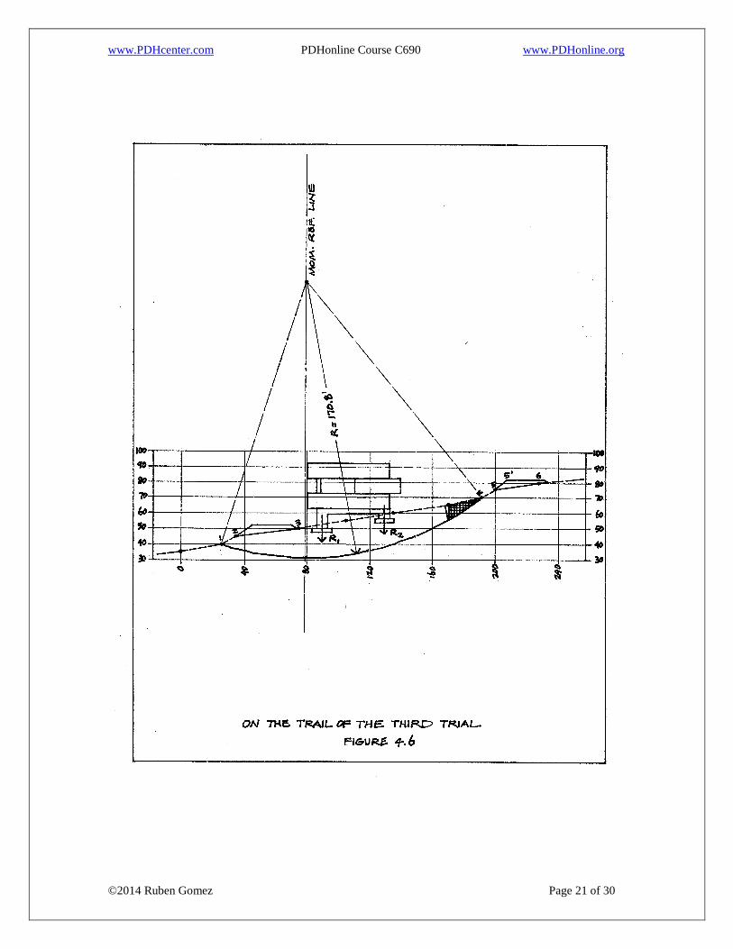
R1 = R2 ≈ 450 kips The first trial was mostly used as a recognizant procedure to gather information, draw the section A-A’ to scale and consider the different alternatives and criteria directed to select the most appropriate sliding surface. For instance, after a closer examination of Figure 4.3, the shaded areas on the profile marked from points 2 and 3, as well as 5 and 6 were expected to be well compacted to at least 100% of maximum density according to the standard AASHO Specification T-180 as commonly required in road construction. Although soil tension cracks were improbable in such areas, however, were predictable in the immediate spots on either side of those compacted areas. We selected point 1 as the possible toe and point 5’ as the probable heel of the expected circular rupture plane. The graphically measured distance from point 1 thru to point 5’ was determined to be 188 ft. Both points were then connected with a straight line (chord) and at half point of its distance, a perpendicular line was drawn. Several radii were tried and 235 ft. was found to be the best alternative for the sought radius. The vertical line originating from the center of rotation and running down through the profile, chord and arc constituted the moment reference line. Figure 4.4 describes a full depiction of such second trial and the corresponding computation chart is shown in Figure 4.5. Such an attempt did produce results that seemed near the critical safety factor sought, however it needed some further verification by working out another trial. As we proceeded, it became evident that a shorter radius would produce a smaller and deeper arc, therefore a third trial was necessary and it was worked out based on a 170.8 feet radius. Figure 4.6 described the virtual circular plane of failure from point 1 thru point 4. The hatched triangular area ending at point 4 represented the volume of clay to the right of the tension crack that would not participate in the predicted soil mass active collapse. Figure 4.7 showed the tabulated computations based on the total collapsed soil mass arbitrarily and conveniently divided in eight slices numbered from right to left from 1 through 8. The fourth column represented the lateral areas of each slice for a total of 2,519 square feet. The sixth column recorded the soil volumes and the seventh column showed the soil weights based on a unit value of 115 pounds per cubic feet. The eighth column recorded the building surcharge as applied to slices #3 and #5. Column ten showed the moments generated by the dead loads; please notice that the forces on the right hand side of the moment reference line generated clockwise (positive) moments

and the forces to the left negative moments, for a resultant moment of 264.8 x 10³ kip-ft. Finally, the fifteenth column gave us the total predicted friction area of 5,800 square feet.

As it came out in retrospect, both solutions brought safety factors that were very close to each other as a clear indication of being in the proximity of the critical safety factor. Before we continue, there are some exceptions we have taken to the commonly accepted modus operandi which need clarification. Many of the methods available to analyze slope failure mechanisms readily accept the principle of slice abstraction as we have done,





however, the proponents of such methods reason that in order to maintain the equilibrium of those slices so conceived as isolated free bodies, they must be bound by stabilizing shear and axial forces. Although that idea is well accepted and conciliated with the known principles of statics we are all taught in school, nevertheless, we should notice that such slicing is a purely imaginary assumption and nothing else. During collapse, the slope is not reduced to a chain sequence of idealized slices, rather, the process is more likely a disintegrating slumped mass on an out swing motion where those so called “inter-slice boundary forces” do not really exist, nor do they contribute in any way to avoid the impending failure mechanism. That is the reason why in our simplified method of analysis we have entirely ignored the presence of such forces. As a second point, the reader has likely noticed that in the chart of Figure 4.7 we have left two blank columns corresponding to the friction resistance as it will not be added to the total capacity of the engaged soil mass. The reason for that is that friction resistance is off-phase with the direct shear as recorded on said chart. Despite the fact that most authors (Bishop, Spencer, et al) support the idea of including frictional shear as a contributor to the factor of safety, that is a debatable assumption. In the opinion of this author, friction and shear resistance do not take place in due synchronicity, and therefore their contributions are not additive. In his view, the mechanism of failure begins with shear failure followed by the development of the circular plane of rupture, followed by friction resistance, in that order. Experiments results as described by Priest and Snyder (May 1987) show the breakaway force as taking place with a 4 second delay with respect to the forces which played a role in the event. Since there is a lack of synchronicity, and until more research is done in that area, we should take the conservative approach of considering them as non additive. As a final point of contention, it should be reminded in here that the design engineer would not be handling a material with the familiar integrity as he finds it in other construction materials such as wood, concrete or steel, it is rather an amorphous soil mass subject to the typical inherent inconsistencies and variability of such material. Therefore, excessive computation refinements are incongruent with reality where we are still dependent and reliant on empirical knowledge, judgment, precedent and experience. For the same reason, in our analysis procedure we have intensively used graphic methods in lieu of mathematical models whenever that was possible. Continuing with the necessary steps to reach conclusive results, the following data has been transcribed from the project’s geotechnical report: Description of the average specimen: Undisturbed grey silty clay. Ultimate soil normal stress: p = 1.0 ksf Soil unit weight: γ = 115 pcf Water content: wo = 18%

Angle of internal friction: Φ = 28°

Cohesion: c = 0.20 ksf Water table: Undetected at 30 ft.





--------------------------------------------------------------------------------------------------------------------- ksf = kips per square foot; pcf = pounds per cubic foot; tsf = tons per square foot --------------------------------------------------------------------------------------------------------------------- With above parameters and using formula (3-2), we may proceed to calculate the soil shear capacity: c = 0.20 ksf p = 1.0 ksf

tan 28° = 0.53

Thus, s = 0.20 + (1.0 x 0.53) = 0.20 + 0.53 = 0.73 ksf From chart in Figure 4.5:

Acting Moment: MDL = 378 x 10³ kip-ft Shear Generated Resisting Moment:

MR = (5,800 x 0.73) 235 = 4,234 x 235 = 995 x 10³ kip-ft

Factor of Safety: FS = 995/3.78 = 2.63 < 3.0 From chart in Figure 4.7: Acting Moment due to DL:

MDL = 264.8 x 10³ kip-ft Shear Generated Resisting Moment:

MR = (5,800 x 0.73) 170.8 = 4,234 x 170.8 = 723.2 x 10³ kip-ft

With the resulting safety factor: FS = 723.2/264.8 = 2.73 < 3.0

































5.0 REMEDIAL SOLUTIONS Our case study has produced a safety factor which can be categorized as being on the low side of desirability and as such, the project could be designated as a low to medium risk case. Nevertheless, it would need attention due to the high possibility of little to no maintenance of the slopes, as it is commonly the case in projects of this nature. As we saw in Section 3.0 under the title “Stabilizing Methods”, there are some measures that can be taken to improve slope safety conditions regarding drainage, erosion control, earth movement and conservation; however, such measures cannot help enough to substantially increase the safety factor to the degree that would be necessary in the case at hand. We will now review other techniques that may assure more effective and permanent results. As suggested before, the assumed sliding surface could be stitched sufficiently to mitigate the possibilities of future failure in slopes of low safety factor design, as pointed out in the accompanied Figure 5.1 by adding features such as drilled piers under the building, tie-backs along the predicted failure plane and a shotcrete applied fungi-form membrane over all or parts the slope. All three systems can be used jointly or separately, according to the merits of the case and to the judgment of the design engineer.









6.0 CHOICE OF TIE-BACK SYSTEMS Amongst a variety of solutions and possibilities, two tie-back anchor systems seem to head the crowd leaving the competition as distant thirds. They are generically designated as grouted anchors and screw anchors. Their names suggest in a large extent what they are and how they work. Grouted anchors basically consist of a drilled hole through the different layers of the soil, followed by the insertion of a continuous steel bar with threaded ends where anchor plates are installed with nuts and washers. The hole, which is recommended to beat least 6 in. in diameter (d), is then pressure grouted to adequately ensure coverage so as to preserve the steel and to produce the necessary friction and thus develop the desired holding capacity. It should be also noticed that an enlarged bulb has been added at the far end of the anchor to increase its capacity against the pull-out forces. A typical detail of a grouted anchor is depicted in Figure 6.1. In our case study it would be appropriate to install the anchors according to a square grid pattern of about 20 x 20 ft. If the total length of the anchor is designated as L, then the distance from the predicted plane of soil fracture (or failure) to the farthest tip into the ground should be anticipated to be at least L/3. The following are the most important characteristics of the grouted anchors: 1- Lower initial cost of (black) steel components. 2- Pre-drilling is necessary. 3- High installation cost. 4- Good performance in high density and rocky soils. 5- When used in loose soils or below water table, the hole may collapse and therefore is requiring encasement. 6- Holding capacity entirely dependent on soil-to-concrete generated friction. 7- Holding capacity predictability entirely based on analytical and/or empirical methods. 8- Longer life expectancy (>30 years). 9- Subject to all the limitations of wet systems, such as heavy equipment access needs; weather condition variables; corrective re-drillings; misalignments; occurrence of underground voids, cavities, caverns and their consequential losses of material. Screw anchors on the other hand, consist of several components, parts and fittings. All such components must be double galvanized to ensure a reasonable performance life. The front piece is furnished with steel helices of adequate diameter which are welded to the main shaft. Helix diameter (D) usually ranges from 4 to 16 in., larger diameters would be impractical for they would require an unreasonable steel thickness. A generic detail of a screw anchor is presented in Figure 6.2 as a detailing reference guide. The same empirical rule of the distance from the predicted failure plane to the farthest tip of the anchor (L/3) also applies. However, in this particular case, that distance





should not be any less than 5D. Use whichever is the longer of the two. A common equation to determine the ultimate capacity of the screw anchor is:

qu = K1C + K2q + 0.33K3Dγ

Where: C = soil cohesion D = largest helix diameter q = overburden loads

γ = soil unit weight K1, K2 and K3 are factors depending on soil shear stress values. The following are the comparative characteristics related to the screw anchors: 1- Higher initial cost of the double hot-dip galvanized steel components. 2- No pre-drilling since the system is capable of self-driving in place. 3- Lower installation cost. 4- Poor performance in high density soils due to the torque limitations of standard rotary equipment. 5- High performance in loose to medium density soils. 6- Dependable holding capacity. 7- Highly predictable holding capacity determined as a function of the recorded driving torque. 8- Limited life expectancy (15-20 years) depending on soil acidity. 9- System can be installed with little interruptions and under very adverse conditions. Just for the convenience of the reader, we present the following Table 6-1 as an “apples-to-apples” and a “head-to-head” comparison of the two herein proposed tie-back systems. Table 6-1 Comparison of tie-back systems

Characteristics Grouted Anchors Screw Anchors

1- Initial cost of components Low High

2- Pre-drilling Needed Self drilling

3- Installation cost High Low

4- Performance in high density soils High Poor

5- Performance in loose soils May need encasement High

6- Holding capacity (HC) Highly dependable Less dependable

7- HC, how determined Empirical methods As a function of driving torque

8- Life expectancy >30 years 15-20 years

9- Installation limitations Affected by prevailing conditions Less affected by prevailing conditions





To finish this section we must add that the shear capacity of the tie-backs (anchors) and drilled piers, at the point where they get crossed by the assumed failure plane, can be added to the overall shear capacity of the soil, which in turn translates into an increase of the safety factor. A regular 6 in. diameter grouted anchor reinforced with a ¾ in. steel bar, is good for an overall shear capacity of 7.5 kips, while a 12 in. diameter drilled pier reinforced with 4 #5 steel bars has a shear capacity of 25 kips. It should be kept in mind however, that those values of shear resistance are subject to the soil having the lateral compressibility to provide the needed support, and therefore, it would be up to the design engineer to make such determination.













7.0 CONCLUSIONS The stability of a natural or even a manmade slope cannot be predicted with an absolute certainty, although as we have seen on the preceding text, a reasonable assessment of an area can be accomplished with a well thought out plan of action coupled with a thorough site investigation. Such an investigation requires a careful analysis of the soil and its groundwater conditions combined with a study of the local geology and a comparative analysis of the existing nearby stable and unstable slopes as well. In that respect, it should be noticed that natural slopes which have remained stable for years and even centuries, may occasionally fail as result of either slow environmental changes or by being accelerated by new construction activities. Consequently, the foundation engineer is cautioned to observe those conditions however subtle, which may bring changes tending to create instability or alter the natural prevailing order of equilibrium. Whenever a hilly area or a given sloping site is being proposed for a new development, both, the proponent(s) as well as the permitting authority should be on the alert to either provide or require the anticipating adequate planning as well as the corrective measures deemed necessary. END



Date post:	02-Feb-2022
Category:	Documents
Upload:	others
View:	4 times
Download:	0 times

Special Foundations Part II - PDHonline.com

Documents