Special Topics: Data Science · Special Topics: Data Science L4b - AR Model Fitting c Prof. Victor...

Special Topics: Data ScienceL4b - AR Model Fitting

c© Prof. Victor Solo

School of Electrical EngineeringUniversity of New South Wales

Sydney, AUSTRALIA

Topics

1 Preliminary Data Analysis.

2 Least Squares Parameter Estimation & Method of Moments

3 Order estimation - AIC,BIC

4 Residuals Analysis/Model Diagnostics

References:Kay, Chapter 5.NotationIn this lecture n ≡ T .

V. Solo (UNSW) ELEC9782 2 / 35

Introduction

We use autoregressive noise models.They only involve linear fitting but are widely applicable.

Basic model fitting is by least squares.

But before fitting one needs to get a preliminary ideaof model structure or pattern.This is best done by looking at plots of acf, pacf periodogram.

After fitting one needs to assess the quality of the fit using modeldiagnostics.


Preliminary Plots

• The first step is to inspect a plot of the data.We look for growth trends, periodicity, amplitude heterogeneity• An amplitude histogram will show skewness.Thus we may decide on data transformation.• Next look at plots of the sample:acf ρr (= Cr/C0); pacf (φrr = πr ); periodogram I (ωk).The acf shows periodicity more clearly than the raw data plot as does theperiodogram, but the periodogram will show this better still.Both acf, pacf help in recognising structure(MA or AR) and order.But acf is noisy and should not be relied on too strongly;the periodogram is also noisy.However successive values of the acf are highly correlated whereassuccessive periodogram values are approximately independent.


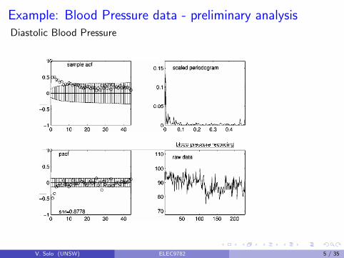
Example: Blood Pressure data - preliminary analysisDiastolic Blood Pressure


Blood Pressure II

We show a plot of the diastolic blood pressure of a subject over a periodof time.Also shown are plots of the sample acf, pacf, periodogram.The bars show ±2 standard error limits.

• We note a slight negative trend but little evidence of amplitudeheterogeneity so no transform seems necessary.• The apparent linear trend shows up in the acf as a slow decay and in theperiodogram as a lot of energy at low frequency.• Since the variance of a physical quantity like blood pressure cannot growwith time we would not believe the time series has a long term trend andso only consider a stationary model.


Preliminary Order Estimation

In the structure estimation stage we try to settle on a few candidatemodels. To do this we have to choose among MA, AR, ARMA as well asthe model orders, then we can obtain parameter estimates, standard errorsand mean square error.Sample acf and MARecall the characterisation of a MA(q) time series, namelyρr = 0, |r | > q

So if the sample acf settles down to near zero after lag q this suggests anMA(q) model is appropriate. By near zero we mean within two standarderrors of zero where the standard error of the acf for a MA(q) model canbe shown to be

se(ρr ) =

√1+2Σq

1ρ2v

n , |r | > qand this is estimated by replacing ρr by ρr . Even armed with the standarderror bars it seems best to use the acf only as a rough guide sincesuccessive values of the sample acf are highly correlated.


Sample pacf and AR

Now recall that an AR(p) time series is characterised by the propertypacfr = φrr = πr = 0 , |r | > p

so if the sample pacf hovers around zero after lag p, this suggests andAR(p) model is appropriate. The sample pacf is much better behaved thanthe sample acf since successive values are approximately independent. Alsothe standard error is simplyse(φrr ) = 1√

n, |r | > p

Example: Blood pressure data - order estimationFrom the plots above we might reject an MA model but entertain anAR(2) or AR(3) (from the pacf).For higher order models or ARMA models these simple methods do notwork very well and so we turn to more automatic methods of orderselection. Such methods require model fitting.


SNR

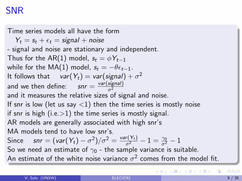
Time series models all have the formYt = st + εt = signal + noise

- signal and noise are stationary and independent.Thus for the AR(1) model, st = φYt−1

while for the MA(1) model, st = −θεt−1.It follows that var(Yt) = var(signal) + σ2

and we then define: snr = var(signal)σ2

and it measures the relative sizes of signal and noise.If snr is low (let us say <1) then the time series is mostly noiseif snr is high (i.e.>1) the time series is mostly signal.AR models are generally associated with high snr’sMA models tend to have low snr’s.Since snr = (var(Yt)− σ2)/σ2 = var(Yt)

σ2 − 1 = γ0

σ2 − 1So we need an estimate of γ0 - the sample variance is suitable.An estimate of the white noise variance σ2 comes from the model fit.


Parameter Estimation - Introduction

Identifiability

Just because a statistical model is written down to describe a set of datadoes not mean it can be estimated; the parameters must be identifiable.

With the Gaussian based techniques we describe, we cannot estimate aparameter if two different values of it can give the same values to the acf.

For MA models for Gaussian data it follows from earlier discussion, theparameters are only identifiable if the MA polynomial is stable (also calledinvertible).

Stable AR models are always identifiable.

ARMA models are identifiable only if both the AR and MA polynomialsare stable.


Parameter Estimation - Least Squares/Linear Regression

The idea here is to reorganise the defining model as a regression and thenestimate the parameters by least squares. This is simplest with the AR.AR by linear regressionRecall the AR(2) model Yt = φ1Yt−1 + φ2Yt−2 + εt , t = 1, · · · , nThis is in fact already a regression model with dependent variable Yt andregressors (Yt−1,Yt−2) which are lagged values of Yt . Because of thelagging we only have regression data for t = 3, · · · , n. The model with amean can be written

Yt − µ = φ1(Yt−1 − µ) + φ2(Yt−2 − µ) + εt

⇒ Yt = µ(1− φ1 − φ2) + φ1Yt−1 + φ2Yt−2 + εt

so the regression intercept is µ(1− φ1 − φ2).For higher order AR models we just include additional lagged Y’s in theregressors.


Example: AR(2) fit to blood pressure by linear regression

The regression fit yields:a fitted mse (σ2) of 16.07 anda fitted snr of .5087.The parameter estimates were (.32,.35) each with standard error .06.The absolute values of the roots of the AR polynomial were (.77,.45) so astable model has been fitted.Stability NoteOne disadvantage of the linear regression approach is that it does notguarantee that the fitted AR polynomial is stable.


Parameter Estimation : Method of Moments

This method uses the equations that relate moments (such as the acf) tothe model parameters.AR(1) by method of momentsFrom the fact that ρ1 = φ we get the estimating equation φ = ρ1

We also know that the AR(1) variance is γ0 = σ2

(1−φ2)and this delivers an

estimator for the noise varianceσ2 = γ0(1− φ2) = C0(1− φ2)

Of course we need standard errors to accompany these estimates. It canbe shown thatse(φ) = se(r1) =

√(1− φ2)/n

and so the estimated standard error will be

se(φ) =√

(1− φ2)/n

Clearly the closer is φ to ±1, the better it can be estimated. For σ2 it canbe shown thatse(σ2) = σ2

√2/n

so that the estimated standard error will bese(σ2) = σ2

√2/n


Higher Order AR models - Yule-Walker Equations

This method extends easily to higher order AR models as follows. For anAR(p) model we write down p equations from the difference equation thatgenerates the acf. But then use the sample acf so,ρr = φ1ρr−1 + ...+ φpρr−p r = 1, · · · , p

These p moment equations ( called the Yule-Walker equations ) can besolved to give estimates of φ1, · · · , φp. In matrix form these equations are

ρ0 ρ1 ... ρp−1

ρ1 ρ0 ... ...... ... ... ...ρp−1 ... ... ρ0

φ1

φ2

...

φp

=

ρ1

ρ2

...ρp

and the inverse of the (Toeplitz) matrix appearing here gives standarderrors when multiplied by σ2.When applied to AR models method of moments guarantees a stationarymodel.


AR(2) fit to blood pressure by method of moments

This gives almost identical results to the linear regression fit.The fit is mainly capturing the low frequency behaviour.

Table: AR(2) fit to blood pressuredata by method of moments.

variance mse snr24.25 16.07 .51

mean se.mean tv89.17 0.46 193.39

phi se.phi tv magn. angle

0.32 0.06 5.22 .77 00.35 0.06 5.64 .45 .5


Order Estimation and Model Comparison by AIC

Most easily developed for the AR case.AR(p) model is Yt = φ1Yt−1 + φ2Yt−2 + ..+ φpYt−p + εtWe can fit this by least squares regression based on data yt , t = 1, · · · ,TBut how to choose p the number of regressors?

Traditional approach is by hypothesis testing.Consider testing for the inclusion of r regressors

Test H0 : p = p0, versus H1 : p = p1 = p0 + d

The F-statistic is: Fd ,T−p1 =s2

0−s21

d /s2

1T−p1

where s2i = RSS after pi regressors are fitted

(RSS = residual sum of squares)


Model Comparison by AIC II

Consider now the F-test acceptance inequality:s2

0−s21

(p1−p0)(s21/(T−p1))

≤ a′

where a′ is an Fd ,T−p1 percentage point. Multiplying the denominatoracross to the right hand side yields

s20 − s2

1 ≤ a′(p1 − p0)s2

1

T − p1⇒ s2

0 ≤ s21 (1 +

a′

T − p1(p1 − p0))

Now take logs (noting that ln(1 + δ) ∼ δ if , δ << 1) to find this isapproximately equivalent to

lns20 ≤ lns2

1 + a′(p1 − p0)

T≡ lns2

0 +a′p0

T≤ lns2

1 +a′p1

T

The expressions on each side of this inequality have the same form.This suggests the following idea: plot the function lns2

p + a′pT as a function

of p to find its minimizer p∗.(as p rises lns2

p falls but a′pT rises so the sum should have a minimum).


Model Comparison by AIC III

If we take p∗ in the null hypothesis then it will always be accepted whentested against any alternative.So p∗ the order we use.

Usually a′= 2 is used so AIC becomes AICp = ln

s2p

T + 2pT .

It proves useful to scale the RSS so AIC is scale free

AICp = lns2p

s20

+2p

T

One can then display each component of AIC as well as AIC itself on thesame plot; they will be of similar sizes.In practice we consider not only the minimal order model but other modelswhose AIC values are close to the minimum.We have ignored the fact that a

′actually depends on p1. But for low order

models a′=2 is equivalent to a nominal significance level of 5-10%.

BIC uses a = ln(T ) so penalises order more heavily.


Blood pressure data - order estimation by AIC/BIC

The figure shows plotsof AIC & BIC for ARmodel order.AIC suggests p = 4;BIC suggests p = 2.In practice residualsanalysis helps make afinal decision.

0 5 10 15 20 25 30 35 40

2.8

3

3.2 AIC-AR(d=0)

min. at 4

Oder estimation for Blood Pressure Data

0 5 10 15 20 25 30 35 40-0.5

0

0.5 BIC-AR(d=0)

min. at 2


Model Diagnostics/Model Criticism/Residuals Analysis

These procedures are similar to residuals analysis in regression.But there are also some methods special to time series.• Inspect plot of the residuals and a histogram.Look for the possible need for transformation, presence of outliers,remaining trends or cycles in the data.A more formal assessment of Gaussianity can be made with the nscoresplot and associated correlation test.• The acf,pacf,periodogram are then inspected.They should show behaviour consistent with white noise (i.e. no structure).The residuals snr should be <<1.A more formal assessment of how well the residuals conform to a whitenoise can be made from the cumulative periodogram with its associatedKolmogorov-Smirnov 95% confidence lines.


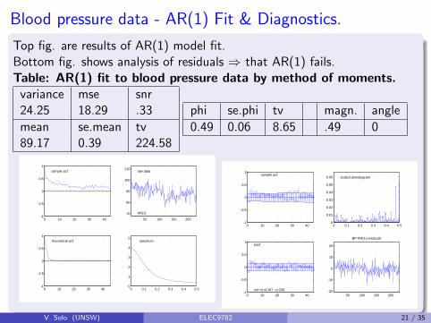
Blood pressure data - AR(1) Fit & Diagnostics.

Top fig. are results of AR(1) model fit.Bottom fig. shows analysis of residuals ⇒ that AR(1) fails.Table: AR(1) fit to blood pressure data by method of moments.

variance mse snr24.25 18.29 .33

mean se.mean tv89.17 0.39 224.58

phi se.phi tv magn. angle

0.49 0.06 8.65 .49 0

50 100 150 20070

80

90

100

110 raw data

AR(1)

0 10 20 30 40-1

-0.5

0

0.5

1sample acf

0 10 20 30 40-1

-0.5

0

0.5

1 theoretical acf

0 0.1 0.2 0.3 0.4 0.50

1

2

3

4

5 spectrum

0 10 20 30 40-1

-0.5

0

0.5

1sample acf

0 10 20 30 40-1

-0.5

0

0.5

1pacf

snr=0.41187, n=230

0 0.1 0.2 0.3 0.4 0.50

0.01

0.02

0.03

0.04

0.05

0.06 scaled periodogram

50 100 150 200-20

-10

0

10

20

BP-AR(1)-residuals


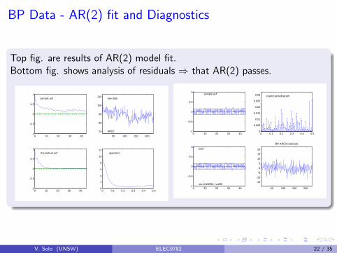
BP Data - AR(2) fit and Diagnostics

Top fig. are results of AR(2) model fit.Bottom fig. shows analysis of residuals ⇒ that AR(2) passes.

50 100 150 20070

80

90

100

110 raw data

AR(2)

0 10 20 30 40-1

-0.5

0

0.5

1sample acf

0 10 20 30 40-1

-0.5

0

0.5

1 theoretical acf

0 0.1 0.2 0.3 0.4 0.50

2

4

6

8

10

12 spectrum

0 0.1 0.2 0.3 0.4 0.50

0.005

0.01

0.015

0.02

0.025

0.03 scaled periodogram

0 10 20 30 40-1

-0.5

0

0.5

1sample acf

0 10 20 30 40-1

-0.5

0

0.5

1pacf

snr=0.24553, n=23050 100 150 200

-15

-10

-5

0

5

10

15

20

BP-AR(2)-residuals


Date post:	27-Aug-2018
Category:	Documents
Upload:	dangnhu
View:	222 times
Download:	0 times

Special Topics: Data Science · Special Topics: Data Science L4b - AR Model Fitting c Prof. Victor...

Documents