SPECIALIZATION: PRO- AND ANTI-GLOBALIZING, 1990-2002
James E. AndersonYoto V. Yotov
Working Paper 16301http://www.nber.org/papers/w16301
NATIONAL BUREAU OF ECONOMIC RESEARCH1050 Massachusetts Avenue
Cambridge, MA 02138August 2010
An earlier version was presented at the NBER ITI meetings, Spring 2010 and the Venice Trade Costsconference, June 2010. We thank participants for helpful comments, especially Keith Head and MichaelWaugh. The views expressed herein are those of the authors and do not necessarily reflect the viewsof the National Bureau of Economic Research.
NBER working papers are circulated for discussion and comment purposes. They have not been peer-reviewed or been subject to the review by the NBER Board of Directors that accompanies officialNBER publications.
Specialization: Pro- and Anti-globalizing, 1990-2002James E. Anderson and Yoto V. YotovNBER Working Paper No. 16301August 2010, Revised April 2011JEL No. F10,F15,R10,R40
ABSTRACT
Specialization alters the incidence of manufacturing trade costs to buyers and sellers, with pro-andanti-globalizing effects on 76 countries from 1990-2002. The structural gravity model yields measuresof Constructed Home Bias (the ratio of predicted local trade to predicted frictionless local trade) andthe Total Factor Productivity effect of changing incidence. A bit more than half the world's countriesexperience declining CHB and rising TFP. The effects are big for the outliers. A novel test of structuralgravity provides striking confirmation, validating both the CHB and TFP measures that rely on it here,and the large gravity literature that relies on it elsewhere.
James E. AndersonDepartment of EconomicsBoston CollegeChestnut Hill, MA 02467and [email protected]
Yoto V. YotovDrexel UniversityLeBow College of BusinessDepartment of Economics and International BusinessMatheson Hall, Suite 503-CPhiladelphia, PA [email protected]
Specialization is revealed in this paper as a powerful force churning the world’s economies
from 1990 to 2002. Trade costs inferred from gravity are large and vary with distance, so the
shifts in the location of production and consumption due to specialization and asymmetric
aggregate growth (described in Section 3 below) must be changing ‘average’ trade costs.
Structural gravity renders this intuition precise in the form of buyers’ and sellers’ incidence
and Constructed Home Bias (CHB, the ratio of predicted local trade to predicted friction-
less local trade) indexes calculated here for 18 manufacturing sectors and 76 countries.1 The
results reveal both pro- and anti-globalizing effects of specialization — some countries have
falling CHB and others rising CHB, all despite unchanging bilateral trade costs. The chang-
ing buyers’ and sellers’ incidence has significant Total Factor Productivity (TFP) effects —
some countries gain while others lose. The effects are big for the extremes.
More important to the large gravity literature, the paper provides a novel test of the
structural gravity model. Its striking confirmation provides important validation for the
incidence measures used here to construct CHB and TFP, and more generally a validation
of applying the restrictions of structural gravity to the gravity model of trade. Structural
gravity forces explain 93% of the variation in country-sector-time-directional fixed effects
estimated from gravity trade flow equations, fixed effects that in principle might be expected
to reflect many other forces.2
The CHB and TFP3 indexes are built on measures of the buyers’ and sellers’ incidence of
trade costs. More than half the world’s countries experience declining CHB and rising TFP
from changing incidence while the remainder of countries experience rising CHB and falling
TFP. Fast growers with rising shares of world shipments tend to experience the biggest
1See Anderson and Yotov (2010) for comparable measures for Canadian provinces.2Earlier gravity model estimation using aggregate trade flows often found GDP coefficient point estimates
differing significantly from the theoretically indicated value of 1. But these findings are not legitimatetests of the structural gravity model because GDP is not the appropriate activity variable and aggregategravity estimation suffers from aggregation bias that substantially understates trade costs, according toour estimates. Moreover, activity variables are perfectly collinear with the fixed effects that control formultilateral resistance, so the earlier estimates suffer from specification bias as well.
3Following the common abuse of terminology, TFP refers here to the Solow residual, not a pure tech-nological change. The structural gravity model implies that the incidence of trade costs is equivalent to atechnology friction, as we show below.
1
declines in CHB (e.g., China’s home bias falls 52% and Ireland’s 47% over the 12 years)
and rises in TFP (China’s TFP rises 18% and Ireland’s 6% ) while unfortunate parts of
the former Soviet Union experience large increases in CHB ( 258% in Ukraine and 109% in
Azerbaijan) and falls in TFP (19% and 42% respectively).4 The correlation between CHB
and TFP ranges from −0.7 to −0.8 depending on the approach used to calculate TFP.
Trade costs are treated as constant in the main account of the paper because the gravity
model coefficients are close to constant in all the variants of the model estimated and dis-
cussed below, and including their inter-temporal variation makes essentially no difference to
the main results. Constant gravity coefficients need not be inconsistent with falling trade
cost levels because the structural gravity model implies that only relative trade costs can
be identified: the bilateral pattern of trade is invariant to uniform proportional changes in
bilateral trade costs (including costs of local shipment).
Section 1 reviews the structural gravity model and its implications to derive measures
of buyers’ and sellers’ incidence of trade costs, CHB and the real output effect changing
incidence of TFP in distribution. Section 2 describes the econometric specification. Section
3 describes the data. Section 4 presents the empirical results. Section 5 concludes.
1 The Structural Gravity Model
Our development follows Anderson (1979) in using the Armington assumption and CES
preferences or technology to derive gravity. It treats the total supply to all destinations and
total expenditure on goods from all origins as exogenous.5
4The churning among the world’s economies revealed here is in sharp contrast to Anderson and Yotov(2010). Their portrayal of Canada’s provinces over the same period uses the same methods we apply here.All Canadian provinces experienced decreased home bias and increased real output as Canada integratedwith the USA and Mexico. The difference is that the present study covers (most) countries in a worldeconomy with both fast (China, India) and slow (Japan) growing and specializing economies.
5The CES-Armington model nests inside many full general equilibrium models characterized by tradeseparability: two stage budgeting and iceberg trade costs ⇒ distribution uses resources in the same propor-tions as production. The weights in the CES preferences or technology can be endogenized with monopolisticcompetition structure (Bergstrand, 1989) while sector supply is determined by Heckscher-Ohlin productionstructure. Eaton and Kortum (2002) derive an observationally equivalent structural gravity setup from ho-
2
Let Xkij denote the value of shipments at destination prices from origin i to destination
j in goods class k. Let tkij ≥ 1 denote the variable trade cost factor on shipment of goods
from i to j in class k, p∗ki denote the factory gate price, hence destination prices are p∗ki tkij.
Let Ekj denote the expenditure at destination j on goods class k from all origins, while Y k
i
denotes the sales of goods at destination prices from i in goods class k to all destinations.
The CES demand function for either final or intermediate goods gives:
Xkij = (βki p
∗ki t
kij/P
kj )1−σkEk
j . (1)
σk is the elasticity of substitution parameter for k and βki is a share parameter. The CES
price index is P kj = [
∑i(β
ki p∗ki t
kij)
1−σk ]1/(1−σk). For deriving TFP implications we think of
all goods as intermediate goods, hence P kj is the unit cost of the bundle of varieties and the
expenditure Ekj is spending bill on intermediate k in j.
Market clearance implies: Y ki =
∑j(β
ki p∗ki )1−σk(tkij/P
kj )1−σkEk
j . Define Y k ≡∑
i Yki and
(Πki )
1−σk ≡∑
j(tkij/P
kj )1−σkEk
j /Yk. Divide the market clearance equation by Y k and use Πk
i .
Market clearance implies that world supply shares equal ‘world’ expenditure shares:
(βki p∗ki Πk
i )1−σk = Y k
i /Yk, (2)
where βki p∗ki Πk
i is the world market quality adjusted price of variety i of good k. In (2) the
CES ‘world’ price index of k is understood to be equal to 1 because summing (2) yields:
∑i
(βki p∗ki Πk
i )1−σk = 1. (3)
The left hand side of (2) is a CES cost or expenditure share for a hypothetical user or
consumer located in the ‘world’ market. Πki is the sellers’ incidence of trade costs, as if all
bilateral shipments bore a uniform incidence.
mogeneous goods combined with Ricardian technology and random productivity draws, a setup extended tomultiple goods classes by Costinot and Komunjer (2007).
3
Now use (2) to substitute for (βki p∗ki )1−σk in (1), the market clearance equation and the
CES price index. This yields the structural gravity model:
Xkij =
Ekj Y
ki
Y k
(tkij
P kj Πk
i
)1−σk
(4)
(Πki )
1−σk =∑j
(tkijP kj
)1−σkEkj
Y k(5)
(P kj )1−σk =
∑i
(tkijΠki
)1−σk
Y ki
Y k. (6)
Since Πki is the sellers’ incidence, tij/Π
ki is the bilateral buyers’ incidence. P k
j generated by
(5)-(6) is called inward multilateral resistance and is also the CES price index of the demand
system. P kj is interpreted as buyers’ incidence because it is a CES index of the bilateral
buyers’ resistances on flows from i to j in class k, the weights being the frictionless trade
equilibrium shares {Y ki /Y
k}. It is as if buyers at j pay a uniform markup P kj for the bundle
of goods purchased on the world market.6 Πki is also called outward multilateral resistance
(Anderson and van Wincoop, 2003).
Measures of ‘market access’ and ‘supplier access’ proposed by Redding and Venables
(2004) are theoretically equivalent to outward and inward multilateral resistance in equi-
librium but do not provide the incidence interpretation nor provide as clear a path to op-
erationalizing the comparative statics of incidence. Their measure of ‘market access’ uses
essentially the same formula as (5) while their measure of ‘supplier access’ uses the CES
price index formula P kj = [
∑i(β
ki p∗ki t
kij)
1−σk ]1/(1−σk). In equilibrium the p∗ki ’s in the CES
price index must in theory satisfy (2), so the measures are theoretically equivalent.7
6{P kj Πki } is the general-equilibrium-consistent aggregate analog to the one-good partial equilibrium in-
cidence decomposition. If the actual set of bilateral trade costs is replaced by tkij = P kj Πki , all budget
constraints and market clearance conditions continue to hold, and factory gate prices and aggregate supplyand expenditure shares remain constant (Anderson and van Wincoop, 2004). The bilateral shipment patternshifts to that of the frictionless equilibrium. This hypothetical general equilibrium plays a role analogous tothe hypothetical frictionless equilibrium in the one good partial equilibrium incidence analysis.
7In practice, the two measures diverge. Redding and Venables estimate a wage equation proportionalto p∗i in our setup in their one-goods-class Krugman model. We think their methods do not adequatelycapture the highly nonlinear interdependence of inward and outward multilateral resistance in (5)-(6), a
4
1.1 Calculating Incidence and Constructed Home Bias
The multilateral resistances in each sector k are solved for given {tkij, Ekj , Y
ki } from system
(5)-(6). The system solves for {Πki , P
kj } only up to a scalar for each class k, so an additional
restriction from a normalization is needed.8 Our empirical procedure is P kUS = 1, ∀k. See
Anderson and Yotov (2010) for more details. None of our main results depend on the
normalization, as we will explain further as needed. Here we note that the trade flow in
equation (4) is invariant to changes in the scalar λ of the preceding footnote.
(4) leads to a useful quantification of home bias that summarizes the effect of all trade
costs acting to increase each country’s trade with itself above the frictionless benchmark,
Eki Y
ki /Y
k.9 Constructed Home Bias is defined by
CHBki ≡
(tii/Π
kiP
ki
)1−σk . (7)
CHB is the ratio of predicted to frictionless internal trade. Two regions i and j with the
same internal trade cost tii = tjj may have quite different CHB’s because ΠkiP
ki 6= Πk
jPkj .
1.2 Trade Cost Incidence and TFP
Trade cost incidence shrinks the returns to national factors of production on both the out-
put and intermediate input sides of value added. The average reduction in national Gross
Domestic Product (GDP) due to the incidence of trade costs affects national TFP just like
national technology frictions do. In contrast, world TFP in distribution from country i ag-
problem that also affects their comparative static experiments. In terms of our setup they estimate a priceequation derived by equating the right hand side of (4) with the right hand side of (1) and solving for(βip∗i )
1−σ = Πσ−1i YiP
σ−1j Ej/Y . They estimate with regressors obtained as the fixed effects of the estimated
aggregated version of trade equation (4). Recognizing that the market access and supplier access variables areco-determined with the wage (factory gate price in our case), they use lagged estimated fixed effects to replacethe contemporaneous variables. They alternatively use two stage least squares with geographic instrumentsfor origin and destination countries to proxy the fixed effects. None of these expedients adequately reflectsthe simultaneity of (5)-(6), in which every geographic exogenous variable in the system co-determines thefixed effect to be estimated simultaneously with every contemporaneous Ej , Yi.
8If {Π0i , P
0j } is a solution then so is {λΠ0
i , P0j /λ}.
9tkij = 1,∀i, j implies P kj = Πki = 1,∀i, j, using (5)-(6).
5
gregates the sellers’ and buyers’ incidences across countries in an index developed here for
perspective.
Suppose, plausibly, that imported (and local) manufactured goods are all inputs into
final goods. The preceding structure justifies analyzing GDP while abstracting from the
details of distribution. It is as if each sector k ships to a hypothetical world market receiving
price pWki = p∗ki Πk
i in each country i. Also, country i buys goods in sector k from all origins
at a price index equal to one on the world market, paying the additional buyers’ incidence
P ki to bring the the bundle home. The GDP function for country i is the maximum value
function g({pWki /Πk
i }, {P ki }, qi, vi) where vi is the national factor endowment vector and qi is
a vector of non-manufacturing goods prices. The combined reduction in GDP due to buyers
and sellers incidence is implicitly defined as the scalar incidence Gi that delivers the same
GDP as does the actual incidence vector {Πki , P
ki }:
Gi : g({pWki /Gi}, ιGi, qi, vi) = g({pWk
i /Πki }, {P k
i }, qi, vi), (8)
where ι is the vector of ones.
Solving for local rates of change Gi, using standard properties of GDP functions,10
Gi = −∑k
wki Πki −
∑k
ωki Pki , (9)
where wki denotes the share of total manufacturing shipments from origin i due to good k
and ωki denotes the share of total expenditure in destination i on intermediate goods class
k, and the circumflex (hat) denotes the percentage change in the multilateral resistance.
(9) is the same formula used in TFP calculations treating −Πki (−P k
i ) as a Hicks-neutral
productivity improvement in output (input) technology. Conceptually Gi measures by how
much manufacturing value added in i changed due to changed incidence of trade costs, all
10Derivatives with respect to output prices are equal to output supplies; derivatives with respect to inputprices are equal to input demands. The Appendix goes into more technical detail behind the derivation of(9).
6
else equal. Call this the TFP effect of changing incidence.
We use (9) to calculate measures of change in manufacturing value added due to the
changing incidence of trade costs using the changes in levels of multilateral resistances (one
for each commodity class, country and year) and the shares of shipments and expenditures
(one for each commodity class, country and year).
With a 12 year time span and discrete data, there are several plausible choices for applying
the basic idea of (9). A fixed weight approach applies some sensible shipment and expenditure
weights, in our case the shipment and expenditure weights for 1996, the middle year of the
panel, and uses the 12 year percentage change in multilateral resistances in (9).
A more elaborate chain weights approach uses arithmetic averages of yearly adjacent
shares for weights and calculates the yearly percentage change in Gj, adding the changes
up to obtain the 12 year cumulative change. In practice, recognizing discrete changes, we
integrate (9) over the annual intervals, hence use differentials of logs on both sides for the
“price” variables. The cumulative effect is thus obtained by exponentiating
ln[Gj(2002)/Gj(1990)] = −∑k
12∑τ=1
wkj (τ)Πkj (τ)−
∑k
12∑τ=1
ωkj (τ)P kj (τ) (10)
Here,
wkj (τ) ≡wkj (2002− τ + 1) + wkj (2002− τ)
2
and analogously for the ω’s. (10), after exponentiation, is a Tornqvist approximation to a
Divisia index of G. The chain weights approach has significant advantages when countries
experience large shifts in their cross-commodity composition of production and expenditure,
as many do from 1990 to 2002.
Like CHB, G is invariant to the normalization used to calculate the P ’s and Π’s in (9)
or (10). This is because any rescaling raises all P ’s proportionally while lowering all Π’s in
the same proportion, the two effects canceling out in (9) and (10).
The TFP effect of national incidence of trade costs given by (8) stands in constrast to a
7
global TFP measure of productivity in distribution. Sectoral TFP friction in distribution is
defined by the uniform friction that preserves the value of sectoral shipments from origin i at
destination prices: tki =∑
h tkihy
kih/∑
h ykih where ykih denotes the number of units of product
class k received from i at destination h, ykih = Xkih/p
∗ki t
kih. The iceberg metaphor captures
the technological requirement that distribution requires resources in the same proportion as
does production, so in product class k it takes tkihykih of origin i resources to deliver ykih to
destination h. tki is a Laspeyres index of outward trade frictions facing seller i in good k.
Aggregate TFP friction for country i is similarly given by ti ≡∑
k,h tki p∗ki y
kjh/∑
k,h p∗ki y
kih.
ti measures the (inverse of the) productivity of distribution from i to the world economy
as a whole. It measures sellers’ incidence only under the partial equilibrium assumption
that all incidence falls on the seller i, while the analogous inward trade cost measure would
measure buyer’s incidence only under the assumption that all incidence fell on buyers.
Our results show that in practice these differences are significant: Laspeyres TFP mea-
sures such as ti and the TFP effect of incidence differ in magnitude and in the case of inward
measures the correlation between them is low.
2 Econometric Specification
Two steps complete the econometric model. First, we approximate the unobservable bilateral
trade costs tkij with a set of observable variables most of which are now standard in the gravity
literature:11
tkij1−σ
= eP4
m=1 βkm lnDISTm
ij +βk5BRDRij+βk
6LANGij+βk7CLNYij+
P83i=8 β
ki SMCTRYij . (11)
Here, lnDISTmij is the logarithm of bilateral distance between trading partners i and j. We
follow Eaton and Kortum (2002) to decompose distance effects into four intervals, m ∈ [1, 4].
The distance intervals, in kilometers, are: [0, 3000); [3000, 7000); [7000, 10000); [10000,
11See Anderson and van Wincoop (2004) for a discussion of trade costs.
8
maximum].12 BRDRij captures the presence of contiguous borders. LANGij and CLNYij
account for common language and colonial ties, respectively. Finally, SMCTRYij is a set of
country-specific dummy variables equal to 1 when i = j and zero elsewhere.13 These variables
capture the effect of crossing the international border by shifting up internal trade, all else
equal. Using the internal trade dummies has the advantage of being exogenous variables that
pick up all the relevant forces that discriminate between internal and international trade. It
also preserves comparability with the specification used by Anderson and Yotov for Canadian
provincial trade.
Next, we substitute (11) for tij into (4) and then we expand the gravity equation with a
multiplicative error term, εkij, to get:
Xkij =
Y ki E
kj
Y k
(tkij
ΠkiP
kj
)1−σk
εkij. (12)
Estimating (12) requires accounting for the unobservable multilateral resistance terms.
Anderson and van Wincoop (2003) use a full information method incorporating (5)-(6). We
use directional (source and destination), country-specific fixed effects, which is easier to im-
plement and also produces consistent estimates. More important, fixed effects do not impose
unitary elasticities on P σ−1j ,Πσ−1
i , Ej, Yi and allow for other unobservable country/product
effects not contained in the theoretical gravity model. We use time-varying, directional,
country-specific dummies to control for the MRs and the E’s and Y’s in the panel estima-
tions. In Section 4.5 below we check for consistency of the estimated fixed effects with the
calculated multilateral resistances and the output and expenditure shares. The results sug-
12Eaton and Kortum (2002) find that, with aggregate data, the estimate of the distance coefficient forshorter distances is larger (in absolute value) than for longer distances. This could reflect several forces.Motivated by transport costs, there could be mode choice switches (surface for short, air for long). But theseswitches could happen differently for different goods, which is particularly important for our disaggregatedstudy, surface for heavy low value goods no matter how long the trip vs air for high value/weight goods evenfor quite short distances.
13It should be noted that we can only identify country-specific coefficients βki in a panel setting, whichhas been used to obtain our main results. Lacking observations for enough degrees of freedom, we have toimpose common cross country SMCTRY coefficients in our yearly estimates.
9
gest that the structural gravity model comes very close to accounting for the actual data
generating process.
Another econometric challenge in gravity-type estimations is the presence of a large
number of zero bilateral trade flows, which cannot be captured by a simple log-linear OLS
regression. Santos-Silva and Tenreyro (2007) show that the truncation of trade flows at
zero biases the standard OLS approach. In addition, they argue that not accounting for
trade data heteroskedasticity in the log-linear OLS regressions produces inconsistent coeffi-
cient estimates. To account for heteroskedasticity and to utilize the information carried by
the zero trade flows, Santos-Silva and Tenreyro suggest estimating the gravity equation in
multiplicative form using the Poisson pseudo-maximum-likelihood (PPML) estimator.
The PPML estimator is used to obtain the main results in this study. However, in order to
test the robustness of our findings, we also experiment with log-linear OLS regressions and the
two-step selection procedure of Helpman, Melitz and Rubinstein (2008, henceforth HMR).
HMR model selection where exporters must absorb some fixed costs to enter a market. Their
model controls simultaneously for unobserved heterogeneity (the proportion of exporting
firms) and for sample selection. Fixed costs provide an economic explanation, given CES
preferences, for the many zeroes found in bilateral trade flows, a feature even more prominent
in disaggregated data.14 Our benchmark model is PPML because the assumptions of the
HMR model, especially the exclusion restriction that permits identification, are controversial,
while evidence on 10-digit bilateral US exports presented in Besedes and Prusa (2006a,b)
shows flickering on and off that is hard to explain if fixed costs are important.
It is encouraging that our main results are robust to the method of estimation.It turns
out that switching methods shifts the gravity coefficients equiproportionately, so that the
implied t’s are shifted equiproportionately (PPML and HMR reduce gravity coefficients in
14Our data contain 38% zeroes in 1990 and 30% zeroes in 2002. The number of zeroes varies across sectors.Naturally, the most pronounced resource sector, Petroleum and Coal, has the most zeroes, 54% in 1990 and47% in 2002. Furniture and Beverage and Tobacco follow with about 50% zeroes in 1990 and about 40%zeroes in 2002. Santos-Silva and Tenreyro (2011) show from Monte Carlo simulations that PPML performswell even when the proportion of zeroes is large and the proportion varies with the regressors.
10
absolute value relative to OLS). Since gravity can only identify relative trade costs anyway,
differences in estimation methods wash out with the nomalizations.
The OLS technique estimates the following econometric specification for each class of
HMR differs by including a volume effect reflecting selection. PPML exponentiates (13).
In (13) Xij,t is bilateral trade (in levels) between partners i and j at time t.15 ηi,t denotes
the set of time-varying source-country fixed effects that control for the outward multilateral
resistances along with total sales Y ki,t. θ
kj,t denotes the fixed effects that control for the inward
multilateral resistances along with total expenditures Ekj,t.
16 The country fixed effects also
reflect the effect of border barriers varying by country, sector and time.
3 Data Description
The data covers 1990-2002 for 76 trading partners. The countries are listed in Data Ap-
pendix.17 Data availability allowed us to investigate 18 commodities aggregated on the
basis of the United Nations’ 3-digit International Standard Industrial Classification (ISIC)
Revision 2.18 To estimate gravity and to calculate the various trade cost indexes, we use
15Even though we experiment with yearly estimations, our main results are obtained from panel data. Asnoted in Cheng and Wall (2005), “Fixed-effects estimations are sometimes criticized when applied to datapooled over consecutive years on the grounds that dependent and independent variables cannot fully adjustin a single year’s time.” To avoid this critique, we use only the years 1990, 1994, 1998, and 2002. It turnsout, however, that the gravity estimates are not very sensitive to the use of alternative lags.
16In a static setting, the structural gravity model implies that the income and the expenditure elasticities ofbilateral trade flows are unity. Olivero and Yotov (2009) show that the income elasticities are not necessarilyequal to one in a dynamic setting.
17Country coverage was predetermined mainly by the availability of sectoral level production data.18The complete United Nations’ 3-digit International Standard Industrial Classification consists of 28
sectors. We combine some commodity categories when it is obvious from the data that countries reportsectoral output levels in either one disaggregated category or the other. Our commodity categories are: 1
11
industry-level data on bilateral trade flows and output, and we construct expenditures for
each trading partner and each commodity class, all measured in thousands of current US
dollars for the corresponding year.
Our focus on specialization as the driving force in the world economy is based on in-
creasing specialization observed in falling correlation between national shares of world man-
ufacturing output and expenditure across 18 3-digit manufacturing sectors and 76 countries
from 1990 to 2002. Table 1 highlights the change in correlation overall and in a few key
sectors. The decrease in total manufacturing correlation from 0.97 to 0.94 (see column 1) is
Table 1: Correlations: Output and Expenditure Shares(1) (2) (3) (4)
Year All Manufacturing Apparel (322) Leather (323) Food (311)1990 0.97 0.94 0.82 1.002002 0.94 0.74 0.70 1.00This table reports correlations between world output and expenditure sharesfor three 3-digit ISIC categories and total manufacturing in 1990 and 2002.
driven by sectors such as Apparel and Leather (see columns 2 and 3). In contrast, increased
specialization has played no role for categories such as Food (see column 4).
Behind the correlation changes are shifts in key countries’ production and expenditure
shares. For example, between 1990 and 2002, China’s share of world manufactures production
rose from 3.1% to 7.6% while Japan’s fell from 19.7% to 13.7%. Differential aggregate
growth plays a role, but specialization within manufacturing induces heterogeneity in the
comparative performance of sectoral shares. Japan’s world share of Beverages and Tobacco
actually rises while its share of Paper Products falls only marginally. China’s global share
of every sector rises but some less than double (e.g. Printing) while others (e.g., Apparel,
Transport) quadruple.
Theoretical trade, shipments and expenditure data should be measured in user prices
but valuation at full user prices is unobservable, so our data has measurement error, with
Food; 2 Beverage and Tobacco; 3 Textiles; 4 Apparel; 5 Leather; 6 Wood; 7 Furniture; 8 Paper; 9 Printing;10 Chemicals; 11 Petroleum and Coal; 12 Rubber and Plastic; 13 Minerals; 14 Metals; 15 Machinery; 16Electric; 17 Transportation; and, 18. Other. A detailed conversion table between ours and the UN 3-digitISIC classification is available upon request.
12
implications discussed further below. We use the CEPII database that gives CIF valuation
of bilateral exports for Xkij. While this is the best we can do, it leaves out the large portion
of other trade costs paid by the users.19 Shipments data do not include the costs other than
CIF margins paid by users, and the expenditures data is constructed from shipments plus
trade data.
In addition, we use data on bilateral distances, contiguous borders, colonial ties, common
language, and industry level data on elasticity of substitution. The Data Appendix provides
a detailed description of the data sources and the procedures used to construct all variables
employed in our estimations and analysis.20
4 Empirical Results
4.1 Gravity Estimation Results
Tables 2-4 report the PPML panel results obtained with robust standard errors clustered by
trading pair.21 Overall, the disaggregated gravity model works well. The gravity estimates
vary across commodities and across countries in a sensible way.
Importantly, we find that the coefficients are relatively stable over time for any given
commodity category — the puzzle of the missing globalization persists even with our novel
ability to include internal trade and thus estimate SMCTRY effects. To measure the move-
ment of our gravity estimates over time, we construct the percentage changes in the yearly
estimates for the period 1990-2002: %∆Θ = 100× bΘ2002−bΘ1990bΘ1990, where Θ is the yearly PPML
gravity coefficient estimate of any of the regressors in our estimations.22 Except for colonial
ties (CLNY) and internal trade (SMCTRY) there is no evidence of intertemporal change
19Anderson and van Wincoop (2004) report on the large and varying internal distribution margins observ-able in aggregate data, but these exclude some important user costs falling on the end purchaser.
20Tables with summary statistics and the data set itself are available upon request from the authors.21Comparison between estimates obtained with and without clustering reveal that the clustered standard
errors are a bit larger. This suggests positive intracluster correlations, as expected.22These indexes, the corresponding standard errors (computed with the Delta method), as well as the
disaggregated gravity estimates for individual years, are available upon request.
13
while for the former the scant evidence is discussed below.
Distance (DIST1-DIST4). Distance is a large impediment to manufactures trade: all
estimated distance coefficients are negative and statistically significant. For most commodi-
ties, we find an inverted u-shape (algebraically) relationship between distance and trade
flows.23 This non-monotonic pattern contrasts with results of Eaton and Kortum (2002),
who report monotonically rising estimates of distance elasticities based on aggregate data.
Distance elasticities vary greatly by sector, consistently with variation in value to weight and
the physical requirements of transportation.
Common Border (BRDR). All estimated coefficients on the contiguity variable BRDR
are positive, large and, in most cases, significant.24 Contiguity effects vary significantly
across commodities. For example, each of the positive contiguity effects for Wood, Metals
and Electric products are more than twice those for Chemical products.
Common Language (LANG). All else equal, sharing a common official language facili-
tates bilateral trade for eleven of the categories in our sample, marginally so in the case of
Rubber and Plastic Products. Insignificant LANG effects are found for more than one third
of the sectors including Leather, Wood, Paper, Petroleum and Coal, Electrical Products,
Transportation and Other Manufacturing products. The variation in the magnitude of the
coefficients across commodities makes intuitive sense. Thus, for example, while the estimate
on Paper is neither economically nor statistically significant, the estimate on Printing and
Publishing is the largest. The explanation is that knowledge of a specific language is nec-
essary for consumption of published products. It is also intuitive that language should not
matter much in the case of Petroleum and Coal, which is the most pronounced resource
sector in our sample.
23The negative effect of distance on bilateral trade is usually smallest for the countries that are less than3000 kilometers away from each other. Depending on the commodity, the effects of distance are largestfor country pairs in either the second interval, of [3000, 7000) kilometers, or in the third interval, of [7000,10000) kilometers. In the case of Chemicals the estimate of the distance coefficient increases (in absolutevalue) with the distance interval.
24The two exceptions are Leather Products, with a positive but insignificant coefficient, and Beveragesand Tobacco Products, for which the coefficient estimate on BRDR is neither economically nor statisticallysignificant.
14
Colonial Ties (CLNY). As compared to the other gravity variables, ‘colonial ties’ is
the regressor with least explanatory power. Tables 2-4 indicate that colonial ties increase
bilateral, commodity-level trade flows only for a few product categories: Only one-third of
the CLNY coefficient estimates are positive and significant, and, in most cases, marginally
so.25 Furthermore, the significant estimates are small in magnitude. Colonial ties matter
most for the categories of Beverage and Tobacco, Apparel, Leather Products, and Printing
and Publishing Products. Overall, our estimates suggest that the effects of colonial ties have
slowly disappeared during the 90s.
Same Country (SMCTRY). International borders reduce trade, all else equal. The co-
efficient estimates reported in Tables 2-4 are averages across all country-specific estimates.
The vast majority of the estimates of the coefficients on SMCTRY (the dummy variable
capturing internal trade) are positive, large, and significant at any level. Beverages and
Tobacco and Printing and Publishing are the two categories with highest domestic bias in
trade, while Machinery and Transportation, are among the categories with lowest SMCTRY
estimates. The high estimates for the former sectors suggest a large relative cost advantage
(e.g., in advertising) to reaching local consumers while the low estimates for the latter sec-
tors suggest that a lower relative cost advantage of reaching local users. The variation of
the estimated SMCTRY coefficients makes intuitive sense at the country level too. First,
less developed nations are more prone to buy domestic products. Thus, Mongolia, Iran
and Tanzania are the three nations with largest average SMCTRY estimates, followed by
Kenya, Senegal and several former Soviet republics including Kazakhstan, Kyrgyz Republic
and Armenia. Second, the regions with lowest bias in purchase of domestic goods are the
Netherlands, Germany, Belgium-Luxembourg and US.26
25Less than one third of the yearly estimates of the coefficients on CLNY are significant. For the fewproducts for which the yearly estimates are significant, we find that the CLNY effects have decreased overtime, but the decrease is not statistically significant.
26We estimate negative average internal trade coefficients for two regions: Hong Kong and Singapore.It should be noted though that the estimates for Transportation and Other manufacturing, where theseregions seem to have comparative advantage are positive (but not significant), while the SMCTRY estimateon Machinery for Hong Kong is positive and statistically significant.
15
Overall, the SMCTRY effects are persistent over time.27 The percentage changes of the
yearly estimates are mostly small in magnitude and not statistically significant. There are
a few categories for which we estimate a significant decrease in the domestic bias over the
period 1990-2002. These commodities are Textiles, Apparel, Metals, and Electrical products.
For Textiles and Apparel, the entry of China into the WTO is an obvious explanation despite
the contrary effect of the MFA, none of which is modeled. Petroleum and Coal products is
the only category for which we find an increase in domestic bias. Possible explanations for
this finding include recent wars and political conflicts, and efforts to improve energy security.
In order to abstract from any effects due to changes in the yearly gravity estimates,28 we
choose to employ the panel PPML estimates in the calculation of the trade costs indexes be-
low. As more justification for this procedure we construct correlations (by product) between
the panel PPML estimates and their yearly PPML counterparts. All correlation indexes are
very large (above 0.9) and significant.29 This suggests that the two estimation sets (panel
and yearly) can be used interchangeably in the calculation of the trade costs indexes.
As a robustness check, we compare the panel PPML estimates against two alternative
econometric specifications, a log-linear OLS and a two-step HMR procedure. Santos-Silva
and Tenreyro (2006) criticize the standard log-linear OLS approach to estimate gravity as
inappropriate. They argue in favor of the PPML estimator and find significant biases in the
OLS gravity estimates. In accordance with their findings, but using disaggregated data, we
find an upward bias in the OLS estimates, especially in the coefficient estimates of distance
and of colonial ties. These results are consistent in both the panel and the yearly estimations.
Importantly for present purposes, there is almost perfect correlation between the OLS (both
yearly and panel) estimates and the PPML gravity estimates. Remembering that the gravity
system identifies only relative trade costs, the very high correlation between the PPML and
27To obtain yearly SMCTRY estimates we impose a common cross-country coefficient for each commodity,because a country-specific indicator trade dummy would have had only one observation that differs fromzero.
28In a few instances, we obtain wrong-sign estimates. For example, we estimate a positive and significanteffect of distance on bilateral trade for Textiles in 1990.
29These numbers, along with the yearly PPML estimates, are available upon request.
16
the OLS estimates suggests that the two sets are equally good proxies for the unobservable
bilateral trade costs and can be used interchangeably for our purposes.
Finally, we compare the panel PPML estimates to estimates obtained with the two-
step HMR method, where exporters must absorb some fixed costs to enter a market. HMR
estimation controls simultaneously for sample selection bias and for unobserved heterogeneity
bias. To keep the sample size as large as possible, we follow HMR in using religion as the
exclusionary variable that permits identification. We apply the HMR cubic polynomial
specification to control for the biases caused by the unobserved firm heterogeneity along
with the Heckman (1979) sample selection correction to obtain both panel as well as yearly
estimates. The disaggregated HMR estimates support their aggregate findings: both the
selection and the unobserved heterogeneity biases are significant, which leads to exaggerated
OLS estimates. But most important for our purposes is the almost perfect correlation
between the panel PPML estimates and the HMR panel and yearly counterparts.30 PPML
and HMR (and OLS) estimates turn out to be essentially equivalent for the calculation of
the trade cost indexes.
4.2 Multilateral Resistance Indexes
The multilateral resistances are calculated from (5)-(6) with fitted bilateral trade costs and
data on expenditure and supply shares. Let τ kij ≡ (tkij)1−σk the power transform of the
bilateral trade cost factor. We construct τ kij from the estimated gravity coefficients , the β’s,
and the proxy variables data as:
τ kij = eP4
m=1bβkm lnDISTm
ij +bβk5BRDRij+bβk
6LANGij+bβk7CLNYij+
P83i=8
bβki SMCTRYij .
Where needed to get the levels of multilateral resistances, σk is the estimate of the elasticity
of substitution obtained, as described in the data appendix, from the 3-digit HS indexes of
30Correlation coefficients and HMR estimation results (panel and yearly) are available upon request.
17
Broda et al. (2006).31
Theory implies that bilateral trade cost factors tkij should always be greater than one.
In less than one percent of the cases (mostly for the estimates of internal trade costs, tkii)
our estimates are lower than one. To preserve the variability in the bilateral trade cost
estimates, we divide each of them by tkij,min, where tkij,min is the smallest estimate for a given
class of commodities (usually the internal estimate for a small country). This transformation
is inconsequential for our analysis since the full gravity system is homogeneous of degree zero
in the set of gravity implied trade costs. Estimation can only identify relative trade costs.
The power transforms of multilateral resistance are solved from the gravity system (5)-
(6) using the τ ’s. Overall, we find significant variation, within reasonable bounds, in the
multilateral resistances across countries for a single product, and across commodity lines for
a given country. For brevity and clarity of exposition, we construct and analyze aggregate
indexes across all commodities for a given nation, and across all countries for a given com-
modity category. We use expenditure shares as weights in the aggregation of the inward
multilateral resistances and output shares in the aggregation of the outward counterparts.
Intertemporal variation is induced by changing shares with constant bilateral trade costs.
To describe the evolution of the multilateral resistances over time, we follow the procedure
from Anderson and Yotov (2010) who adopt a time-invariant normalization to convert cur-
rent prices to base year prices. Applied to our setting, the procedure is to convert US current
inward multilateral resistance (chosen for normalization) to base year US inward multilateral
resistance. Initially we calculate MR’s for each commodity with PUSA(t) = 1 for each year
t. This yields (for each commodity) a set {Pi(t),Πi(t)} for each region i and year t. Using
output and expenditure shares, respectively as weights, we aggregate commodity level mul-
tilateral resistances to form country MR’s. To convert them to intertemporally comparable
values, we construct an inflator variable for US, drawn from country-level personal consump-
31Estimates of σ can be obtained directly as coefficients on bilateral tariffs in the gravity model. However,due to unavailability of bilateral tariff data for the period of investigation, we choose to use the elasticityindexes from Broda et al. (2006)
18
tion expenditures (PCE) prices on durable and nondurable goods (but not services) for the
period 1990-2002.32 The inflator is equal to πUSA(t) = PCEUSA(t)/PCEUSA(1990). The new
set of ‘time-consistent’ MR’s is {πUSA(t)Pi(t), (1/πUSA(t))Πi(t)}. Conceptually, any coun-
try’s inward MR is converted to a 1990 US dollars equivalent. For example, Pi(t)/PUSA(t)
is replaced by Pi(t)/PUSA(1990). The scale of outward MR’s is inversely related to the scal-
ing of inward MR’s due to the structure of the gravity system, so outward MR’s are also
interpreted as being in 1990 US dollars.
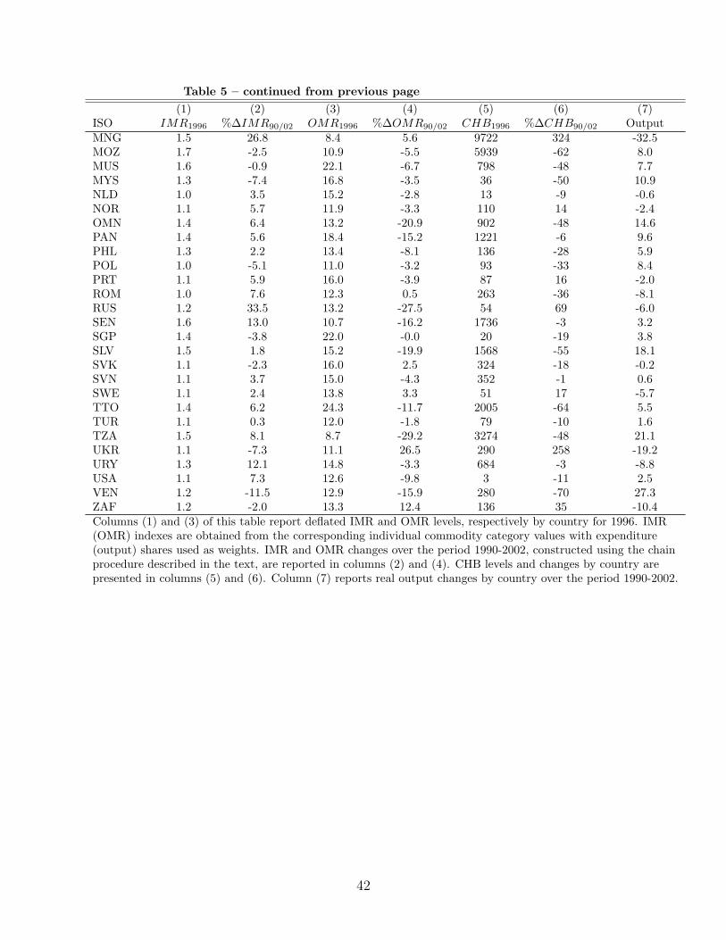
Deflated inward multilateral resistance (IMR) indexes are reported in Table 5. Column
(1) reports IMR’s by country for 1996, the midyear of our sample that is also representa-
tive.33 The IMR values vary across countries, and the pattern of IMR variation makes good
intuitive sense. More ‘remote’ nations, geographically and in terms of industry concentra-
tion and economic development, face larger buyers’ incidence. Thus, developing countries
(e.g. Mozambique, Senegal and Tanzania) and some former Soviet republics (e.g. Kyrgyz
Republic and Azerbaijan) are consistently among the regions with highest buyers’ incidence.
In contrast, all developed countries are in the lower tail of the IMR distribution. The levels
and range of values of IMR’s in manufacturing for countries resemble those for Canada’s
provinces over a wider set of goods in Anderson and Yotov (2010).
The numbers in column (2) of Table 5 summarize the IMR changes over the period 1990-
2002 and are constructed using the chain procedure of Section 1.2. Over time consumers
in twenty eight of the countries in our sample enjoyed a moderate decrease in the inward
multilateral resistances. Consumers in the Czech republic and Indonesia are the biggest
winners. On the opposite side of the spectrum of IMR changes we find Russia, with an IMR
increase of 34 percent, and another former Soviet republic, Azerbaijan, with an even larger
increase of 55 percent. The estimates for these two nations are in accordance with the fact
that they are among the countries with largest consumer price increases in the sample.34
32The PCE price index is constructed and maintained by the Bureau of Economic Analysis.33These numbers are the deflated yearly average inward multilateral resistances for each country across
all goods, weighted by the national expenditure share on each commodity.34In principle, IMR changes are comparable to average CPI changes. However, IMR’s may only loosely
19
IMR’s vary across product lines for a single country. We aggregate across countries
to portray the cross-commodity variation of the IMR’s in Table 6. The numbers for each
year and commodity are calculated as relative to the corresponding number for the United
States. Thus, the indexes from column (1) of Table 6 suggest that the average consumer
costs of Food, Wood, and Paper Products are considerably higher in the rest of the world,
as compared to the US, while the average costs of Furniture, Apparel and Mineral Products
are lower than in the US.
Estimates of the percentage changes in the IMR indexes, reported in column (2) of
Table 6, show that, on average, the inward multilateral resistances have increased for most
commodity categories (about two thirds) in our sample. The increase varies by product line.
At 12%, Food and Furniture are the categories for which consumers have suffered the largest
IMR increase over the period 1990-2002. Rubber and Plastic and Electrical products are
two other sectors with large IMR increase. Wood and Beverage and Tobacco are two of the
categories with IMR decrease of more than 10%. Petroleum and Coal is the category with
largest IMR fall of 22%. This finding coincides with the stable oil prices of the 90’s, followed
by a fall in the early 2000’s, and the fall in IMR’s due to changing specialization patterns
may be part of the explanation.35
Outward multilateral resistance (OMR) indexes for manufacturing also vary across in-
dustries for a single country and across nations for a single sector. Once again, to ease
interpretation of our findings, we aggregate OMR’s across commodities for each country and
across countries for each commodity using commodity shipment shares as weights. The vari-
ation of the OMR’s across countries is revealed in column (3) of Table 5, where we report
track variations in consumer price indexes and any differences between the CPI’s and the IMR’s have anumber of explanations. First, our IMR indexes are based on a manufacturing sample, excluding services,agriculture and mining. Second, the inward incidence of trade costs probably falls on intermediate goodsusers in a way that does not show up in measured prices. Third, the production weighted IMR’s are notreally conceptually comparable to the consumer price indexes of final goods baskets. Next, home bias inpreferences may be indicated by our results. Home bias in preferences results in attributions to ‘trade costs’that cannot show up in prices. Finally, the IMR’s are no doubt subject to measurement error and are basedon a CES model that itself may be mis-specified.
35The oil price fall is also partly explained by a series of increases in OPEC quotas, increase in the Russianproduction, and a weakened US economy. Prices fell further immediately after the September 11 attacks.
20
deflated outward multilateral resistances for 1996. In column (4) of the table, we calculate
the percentage change in the OMR’s over the period 1990-2002 using the chain procedure of
Section 1.2. Overall, the levels and range of values (7.8-31.9) are significantly higher than
for Canada’s provinces (3.5 to 7.6) in Anderson and Yotov (2010). This is also consistent
with the relatively low aggregate OMR for Canada reported in Table 5. The explanation is
that the largest trading partner for each Canadian province and territory, or for Canada as
a whole, is very close geographically and trade between Canada and US is ‘free’.
The pattern of OMR variation makes good sense for the most part. Three properties
stand out. First, the regions with the largest sellers’ incidence are more remote regions
(geographically and in terms of industry concentration and national specialization) and some
former Soviet republics. Interestingly, we find that the regions with lowest OMR’s are also
less developed economies such as Iran, Mongolia, Kenya and Tanzania. The reason is that
these regions have the largest SMCTRY estimates, tending to lower their OMR’s. Mexico
also a low OMR, due to its large trade with US, fostered by NAFTA and free trade relations
with the EU and series of Latin American countries during the period of investigation.
As expected, we find the majority of developed countries in the lower halve of the OMR
distribution. Second, OMR’s are considerably larger than the IMR’s, as in Anderson and
Yotov (2010).36
Third, we find evidence of a decline over time in the OMR’s for close to two-thirds of the
nations in our sample and an increase in the seller’s incidence for the rest of the countries.
See column (4) of Table 5. This stands in sharp contrast to the uniform OMR fall for
36To explain why the outward multilateral resistance exceeds its inward counterpart, they draw intuitionfrom two propositions. According to Proposition 1, larger supply or net import shares (defined as thedifference between expenditure shares and output shares) tend to reduce multilateral resistances in a specialcase. Building on the intuition from Proposition 1, in Proposition 2 they show that a greater dispersion ofsupply shares, which is an empirical regularity, drives average outward above average inward multilateralresistance. This pattern also plausibly reflects specialization, with causation running from multilateralresistances to supply (and demand) allocations. The prediction of Proposition 1 holds up strikingly well inour OMR estimates, helping to explain some other results as well. Correlations between the OMR’s andthe output and net import shares at the product level, available upon request, reveal that the OMR’s aresignificantly decreasing in output shares and decreasing in net import shares.
21
Canada’s provinces in Anderson and Yotov (2010).37 Essentially this reflects the empirical
regularity that OMR decreases with supply shares and the zero sum property of changes in
shares. Specialization in the global economy induces incidence shifts that cause gainers and
losers, especially via sellers’ incidence. The Canadian provinces turn out to be a specially
favored case with the zero sum aspects of their interaction inflicted on the much larger
outside world. Kuwait is the nation experiencing the largest OMR increase of close to 32
percent. The reason is the large increase in the incidence on the producers of Petroleum and
Coal (Multilateral resistance and output changes for individual commodities are available
upon request). Most of the oil producers in the world also suffered OMR increase, but the
oil industry accounts for more than 85 percent of Kuwait’s exports and for more than 50
percent of its GDP, extreme relative to other oil exporters.
Sellers in some republics from the former Soviet bloc (e.g., Armenia, Russia and Kaza-
khstan) enjoy significant OMR decreases, while producers in other Soviet nations, such as
Ukraine, and economies under the heavy Soviet influence, such as Bulgaria, suffer large in-
creases in seller’s incidence. The explanation is that after the collapse of communism, during
the early ’90s, some nations lost their guaranteed portion of the large Soviet market to more
competitive producers, while others expanded into new markets including some in the former
Soviet Union.
The patterns of OMR variation across commodity categories and their change over time
are revealed in columns (3)-(4) of Table 6. Column (3) reports deflated aggregates obtained
with output shares used as weights. Leather, Petroleum and Coal and Other Manufacturing
are always among the categories with highest outward trade costs at the country level,
which translates into high aggregate indexes for these categories. Transportation Products
and Food are consistently among the sectors with lowest OMR indexes. Results from column
(4) of Table 6 indicate that over the period 1990-2002 OMR’s have fallen for more than two-
thirds of the commodities in the sample. Food is the category for which producers have
37It should be noted that we do estimate and aggregate OMR fall for Canada, which is consistent withthe results from Anderson and Yotov (2010).
22
enjoyed the largest OMR fall of more than 12 percent. Beverage and Tobacco and Wood
are two of the categories with largest OMR increase. Petroleum and Coal is the outlier with
OMR increase of 22 percent.
Comparison between the changes in the incidence on consumers and producers at the
product level reveals two interesting patterns. First, any IMR fall is inevitably accompanied
by an OMR increase. And, second, the changes in the corresponding inward and outward
multilateral resistances for each category are almost equal in absolute value. This finding
reflects the formal property of (5)-(6) that the Π’s and P ’s are inversely related on average.
This nearly zero sum result is also captured by the real output numbers reported in column
(7) of the table, discussed below.
The MR characteristics are in sharp contrast to those of Laspeyres trade cost (LTC)
indexes. Share-weighted Laspeyres indexes of bilateral trade costs for each country and year
are constructed as follows. The outward index is calculated as∑
k Tki Y
ki /∑
k Yki , where
T ki ≡∑
j tkijX
kij/Y
ki . The inward counterpart calculation is
∑k T
kj E
kj /∑
k Ekj , where T kj ≡∑
i tkijX
kij/E
kj . The inward and the outward LTC’s (available on request) are very similar
and the same is true for their evolution over time. There is a significant positive correlation
between the OMR’s and both outward and inward LTC’s. In contrast, there is a weak
correlation (sometimes negative) between inward multilateral resistance and either of the
LTC measures. Despite the high correlation of the OMR’s and the LTC’s, the magnitudes
are different. This difference has important resource allocation and TFP implications. An
even more important difference between LTC’s and multilateral resistances is that LTC’s
are flat over time. The pro- and anti-globalizing effects of specialization driving changes in
the multilateral resistance indexes have a nearly zero-sum effect on the global efficiency LTC
measures.
23
4.3 Constructed Home Bias
Constructed Home Bias (CHB) is calculated from (7) using the power transforms of esti-
mated t’s and multilateral resistances for each commodity and country. In practice tkii is the
estimated internal trade cost for country i and commodity k relative to the smallest internal
trade cost for commodity k across all countries and regions. It is important to note that
CHB is independent of the normalization, and of elasticity of substitution estimates because
it is constructed using the 1− σk power transforms of t’s, Π’s and P ’s.
Aggregated country level CHB indexes,38 are obtained as weighted averages across com-
modity level CHB values. Recalling that CHB is interpreted as the predicted value of internal
trade relative to the theoretical value of internal trade in a frictionless world, the aggregate
CHB for country or region i should be the ratio of predicted internal total trade∑
k Xkii to
frictionless internal total trade∑
k Yki E
ki /Y
k. This can be obtained from (7) as:
CHBi =∑k
(tkii
ΠkiP
ki
)1−σk Y ki E
ki /Y
k∑k Y
ki E
ki /Y
k,
the weighted average of commodity CHB’s, where the weights are equal to the frictionless
internal trade shares.
Column (5) of Table 5 portrays the cross-national variation of CHB in 1996, which is
representative of our findings across the whole period 1990-2002. Three properties stand
out. First, most of the CHB values are large. There is a massive home bias in trade
flows. Second, there is wide variability in CHB. Third, CHB is larger for the less developed
and the smaller countries, and lower for the more developed and the industrialized nations.
Thus, in each year, the United States (USA), Japan (JPN), Germany (DEU) and France
(FRA) are consistently the four countries with the lowest constructed home bias indexes.
On the opposite side of the CHB spectrum are developing and small countries such as
Mongolia (MNG), Mozambique (MOZ), Tanzania (TZN) and Trinidad and Tobago (TTO),
38CHB indexes at the product level for each country are available upon request.
24
as are most of the former Soviet republics. Compared to the CHB’s for Canadian provinces
reported in Anderson and Yotov (2010), the range of CHB’s is contracted substantially,
explained because countries are more diverse in size than provinces.
The CHB changes over the period 1990-2002 are entirely due to the general equilibrium
effect of changes in production and expenditure shares on multilateral resistance. A fall in
CHB is not due to the usual understanding of globalization because the fitted trade costs
tij’s (including the internal fitted values tii’s) are constant over time by definition, as we
employ the panel (time-invariant) gravity estimates to construct them. Specialization drives
pro- anti-globalization, both falling and rising CHB.39
Column (6) of Table 5 reports percentage changes in CHB for each country and region
in our sample. From 1990 to 2002, CHB falls for about two-thirds of the countries while
rising for the rest. The pattern is mostly explained because market share tends empirically
to lower outward multilateral resistance. Slower than average growth implies smaller market
shares that are associated in the cross section with higher outward multilateral resistance.
The more developed and industrialized economies, which in the 90’s are already pretty well
set in their specialization patterns, do not experience large CHB changes. Thus Germany,
Great Britain, and France are in the middle of the distribution of CHB changes. Notably,
US experiences a moderate fall in CHB, while, in contrast, Japan experiences a large CHB
increase. This is likely due to its lost decade of slow growth in the 90s.
The mixed CHB change results here stand in contrast those of Anderson and Yotov
(2010), revealing falling CHB for all of Canada’s provinces over a wider set of goods. The
difference in results is due to differences in the drivers in each case, the changes in supply
and demand shares. We make no attempt here to endogenize supply and demand shares but
note that incidence would play a role along with other familiar forces of specialization and
39To assess the relative importance of specialization vs. changes in bilateral trade costs, we constructan alternative CHB measure, where we employ the yearly gravity estimates to calculate fitted trade costs.Comparison between the CHB changes obtained with the panel and the yearly gravity estimates reveals thatthey are almost identical. Thus, the CHB fall is indeed due to the general equilibrium effect of changes inproduction and expenditure shares on the multilateral resistances, and the usual forces of globalization haveplayed a small role for the CHB changes during 1990-2002.
25
growth.
The newly liberalizing economies are at the upper tail of the distribution of CHB changes.
For example, Mexico and China are among the nations experiencing large CHB falls. Some
of the smaller European economies, such as Portugal and Greece, that have not gone through
serious economic changes during the period 1990-2002, experience an increase in CHB. Fi-
nally, the big changes in former Soviet bloc trade had different effects on the CHB for the
Soviet republics. Most of them suffered a significant CHB increase. Notably, three of the
five countries with largest CHB increase are the Kyrgyz Republic, Ukraine and Azerbaijan.
The fourth is Bulgaria, which was heavily influenced by the Soviet Union. In contrast, some
former Soviet nations (e.g., Estonia, Latvia and Armenia) enjoyed CHB fall.
CHB’s vary across product lines for a single country. The patterns of CHB variation
across commodity categories and their change over time are revealed in columns (5) and (6)
of Table 6. Notably, we find that product-level CHB indexes are relatively small and much
more homogeneous as compared to their country-level counterparts. The explanation for
the small magnitude is that larger and more developed countries, that have very low CHB
values, are given higher weight (due to their size) in obtaining the aggregate CHB indexes
for each category. Even though CHB variation across product lines is not large, it makes
intuitive sense for the most part. For example, we estimate large home biases for Food and
Beverage and Tobacco, which we believe are demand-driven, and for Petroleum and Coal
and Mineral Products, which we explain with the nature of production and supply.40 The
low CHB values for the more technologically-oriented sectors (e.g. Machinery, Electrical
products, Transportation and Other Manufacturing) are also intuitive and can be explained
with clear world specialization patterns in these manufacturing sectors. Finally, we estimate
an average CHB for only five of the commodities in our sample and decrease for the rest. The
40In particular, even though Petroleum and Coal and Mineral Products are natural resource sectors andone may expect low home biases for these categories, it should be remembered that our data covers trade andproduction of manufactured products, which often are produced domestically from crude natural resourcesthat are imported, however our data does not cover natural resource trade flows. This also explains therelatively large gravity estimates of the SMCTRY coefficients, capturing internal trade, for Petroleum andCoal and Minerals.
26
CHB increase is the largest for Petroleum and Coal and Electrical Products, while leather
and Furniture experience the largest fall.
4.4 The TFP Effect of Incidence
Changes in the incidence of trade costs impact manufacturing value added like TFP changes:
real manufacturing output changes. The real output changes in the last column of Table 5,
are constructed using the chain procedure of Section 1.2. It is important to note that our
results for real output changes are independent of (i) the normalization used to calculate the
multilateral resistances, and (ii) the choice of a price deflator (if any) used to intertempo-
rally link the multilateral resistances. In contrast, the results are sensitive to the choice of
elasticity of substitution in each sector, and the division of gains/losses between buyers and
sellers does depend on the external price deflator.
Buyers in most countries suffered increasing incidence of trade costs (column 2), while
sellers in about two thirds of the nations have enjoyed lower incidence of trade costs (column
4). The changes in real output, in column 7, suggest that more than half the world’s countries
experience rising real output while the remainder of countries experience falling real output.
Globalization as specialization generates winners and losers, tending toward a zero sum.
The pattern of real output changes makes intuitive sense for the most part. In the cross
section, and over time, sellers’ incidence tends to fall with increases in output shares.41 Thus,
nations that have been heavily involved in trade (and wider economic) liberalization during
the 90s, such as China and Mexico, are among the countries with largest real output gains.42
Disaggregated real output changes (available upon request) reveal that these nations are
consistently among the countries with largest real output gains at the commodity level. We
also find that some less developed nations and economies in transition enjoy TFP gains as
41See Anderson and Yotov (2010) for more evidence and some theoretical insight.42Venezuela is another example of a country that liberalized trade intensively during the 90s. Moreover,
oil accounts for only one third of Venezuela’s GDP, while manufacturing, which accounts for about one fifthof GDP, has been growing steadily at very high rates. These characteristics explain Venezuela’s high realoutput benefit from the incidence of TFP in distribution.
27
well, which are driven mostly by decreasing average trade costs incidence on producers.
Most of the countries that suffer large real output decline during the 90s are some de-
veloped nations, but mostly economies in transition and members of the former Soviet bloc.
In the case of the latter (see Russia for example) producers often enjoy significant decrease
in outward multilateral resistance, however, the loss for consumers is even larger. These
findings are supported at the commodity level as well. Along with the developing economies
and the economies in transition, some developed nations, led by Japan, also experienced
large real output loss. The explanation is that Japan suffered a lost decade of slow growth
in the 90s. Most of the other developed nations are in the middle of the real output changes
distribution.
For some nations, the real output effect of globalization is quite heterogeneous across
sectors. For example, Brazil enjoyed the third largest real output gain (after China and
Hong Kong, but in front of Italy) for leather products in the world. This is consistent with
the fact that Brazil is one of the world’s largest leather producers and it gained significantly
from the geographical redistribution of the leather industry during the early 90s. More
interestingly, Brazil is the leader in real output gains in the Petroleum and Coal industry.
Brazilian consumers benefitted from falling oil prices during the 90s. Brazilian oil producers
however, were some of the few in the world that actually enjoyed a fall in outward multilateral
resistance. Brazil’s share of world production rose due to the opening of the oil sector to
private and foreign investors during the late 90’s.
While globalization as specialization generates clear winners and losers at the country-
level, our estimates reveal no significant real output changes for the world economy at the
product-level over the period 1990-2002. See column (7) of Table 6. The most significant
gains are realized in the Food, Minerals and Textiles categories. The overall real output
effect for all manufacturing in the world economy is 0.3%. In principle, the shifts in output
and expenditure shares could significantly raise this measure of world efficiency, as on a
smaller scale Anderson and Yotov (2010) argued was the case for Canada’s provinces, due
28
to expenditure on average rising where inward trade costs are relatively low and similarly
supply rising where outward trade costs are relatively low.43
Openness is positively associated with growth in our sample, as changes in CHB and
changes in the incidence of TFP have a correlation coefficient varying between −0.7 and
−0.8, depending on the approach used in the calculation of real output changes.44
4.5 Testing Structural Gravity
Structural gravity theory implies that the sum of the origin and destination country fixed
effects ηki,t + θkj,t estimated from equation (13) should be equal to the structural gravity term
ln [Ekj P
kjσk−1
Y ki Πk
iσk−1
/Y k]. A simple measure of the goodness of fit of structural gravity is
based on the residuals
rkij,t = ηki,t + θkj,t − ln [Ekj,tP
kj,t
σk−1Y ki,tΠ
ki,t
σk−1].
Since the ηki,t + θkj,t variables are estimated as deviations from the US, the composite variable
ln [Ekj P
kjσk−1
Y ki Πk
iσk−1
] is also constructed as a deviation from the US value. In principle
differencing from the US cancels out the global scaling variable 1/Y kt that is otherwise a
component of the structural gravity term. The data points are very densely clustered about
zero in Figure 1 showing the kernel density estimated distribution of the r’s.
The structural gravity term theoretically predicts the fixed effects. The simple R2 of
structural gravity theory is 0.9.45 Considering the amount of sector-country-time variation
43Totally differentiate (5)-(6), multiply by si ≡ Yi/Y and bj ≡ Ej/Y respectively and sum over countries.
Rearranging the results:∑
i(si +∑
j wij)Πi +∑
j(bj +∑
iwij)Pj = 11−σ
(∑i,j wij bj +
∑i,j wij si
),
where wij = sibj(tij/ΠiPj)1−σ and
∑i,j wij = 1. In the frictionless economy, the right hand
side is equal to zero because the sum of shares is equal to 1. Elsewhere, the right hand sideis negative as b’s tend on average to rise where the composite trade friction term is large(i.e., tij/ΠiPj is small), and as s’s tend on average to rise where the composite trade frictionterm is large (tij/ΠiPj) is small.
44The correlation indexes obtained with the chain-type output numbers are larger. Furthermore, if weeliminate the outliers with CHB indexes above 1000, the correlation between the changes in CHB and thechanges in the incidence of TFP varies between −0.8 and −0.85.
45The R2 of structural gravity is given by 1 − V (r)/V (η + θ), where V (x) denotes the variance of the
29
in the fixed effects and in the constructed structural gravity terms this goodness-of-fit is
astonishing.46 Our prior beliefs were far more pessimistic. The standard decomposition of
variance (using the theoretical coefficient of 1 on the structural gravity components) implies
that the multilateral resistance terms ln(ΠkiP
kj ) account for 32.3% of the variance of ηki,t+θ
kj,t’s
while the size effect terms ln(Y ki E
kj ) account for 57.7%. That size effects should matter is
hardly a surprise based on the large atheoretic gravity literature preceding structural gravity,
but the large importance of the multilateral resistance term, arising strictly from structural
gravity, is striking.
The fit of structural gravity improves still more by regressing the rkij,t’s on sector-time
fixed effects to control for differing sector-time mean measurement error in the E’s and Y ’s.47
In addition, to allow for time-varying, country-specific border barriers not modeled in (13)
due to lack of data, we add time-varying country fixed effects:
ηki,t + θkj,t − ln [Ekj,tP
kj,t
σk−1Y ki,tΠ
ki,t
σk−1] = α0 + ψkt + φi,t + ekij,t (14)
The right hand side fixed effects in the estimate of (14) account for 25% of the variance.
Adding the additional explained variation to that of the simpleR2, structural gravity explains
92.8% of the variation in the estimated sector-country-time fixed effects ηki,t + θkj,t.
To probe the robustness of this finding we look suspiciously at time and country effects.
As to time, the estimated ψkt ’s and φi,t’s do not vary much over time, so the structural
gravity term ln [Ekj P
kjσk−1
Y ki Πk
iσk−1
] absorbs essentially all time variation in the directional
country-time fixed effects. To test this further, we experiment by breaking the sector-time
random variable x. The R2’s at the sectoral level are all above 0.9 for all categories except Beverages andTobacco, Apparel, Leather Products and Petroleum and Coal Products all of which have R2 of about 0.8.
46The vast majority of the fixed effects are very precisely estimated. At the same time they vary quite abit across countries and across commodities.
47The estimated ψkj,t + φki,t values can be rescaled as factors that shift trade flows of the gravity equationin levels, obtained by exponentiating. These range from around 0.26 to 1.73, plausibly associated withsector fixed effects on the following reasoning. Suppose, plausibly, that the mean measurement error for eachgoods class k is in proportion to the observable component of global shipments. The range of the estimatedcountry-time fixed effects values is comparable to the range of values implied by the total shipments dataY k/[
∑k Y
k/N ] where N is the number of sectors. This is (0.07, 2.51) and is stable over time.
30
and the country-time dummies into separate year, country and product fixed effects to find
that none of the year dummies are quantitatively significant, and the two year coefficients
that are statistically significant (for 1991 and 1993) are only marginally so.48
As to country effects, results are robust to eliminating country fixed effects (φi,t = 0)
that might control for activity elasticities not equal to one or other country-specific effects
not explained by structural gravity. The R2 of this variant of (14) falls to 0.19. Figure 2
illustrates. The x-axis shows the rkij,t’s and the y-axis shows the fitted residual values, the
ekij,t’s of (14). If neither sector-time nor country fixed effects mattered, the points would
lie on the 45 degree line. The 95% confidence band of the fitted line for (14) contains the
line labeled “Fitted Values No Country FEs” that plots the fitted values of (14) estimated
subject to φi,t = 0.49 Even the 45 degree line is mostly contained in the confidence band,
emphasizing the minor role of all the fixed effects in (14) in improving the fit of structural
gravity. The data points are very densely concentrated in the center of Figure 2, as indicated
by Figure 1.
As a useful exploration of the performance of structural gravity we also estimate
ηki,t + θkj,t = γk0,t + γk1,t ln [Ekj,tP
kj,t
σk−1Y ki,tΠ
ki,t
σk−1] + εkij,t (15)
for each k and t, and overall. Here εkij,t is a random error term that is correlated with
measurement error in ln [Ekj,tP
kj,tσk−1
Y ki,tΠ
ki,tσk−1
]. The standard test for estimated γ1 6= 1 is
therefore invalid because the estimator is biased. Measurement error in the structural gravity
term is due to the activity variables {Y ki , E
kj } both directly and in calculation of multilateral
resistance in (5)-(6), along with the usual estimation error from the gravity coefficients, both
of which are correlated with estimation error in the ηki,t + θkj,t’s.50
48Full details are available on request.49For visual clarity, the data range is truncated to exclude an outlying 1.3% of dependent variable obser-
vations. About 1/4 of the country-time fixed effects are not statistically significant, although the F-test forjoint significance rejects the null hypothesis for country-specific fixed effects.
50Theory assumes shipments evaluated at full user prices whereas actual shipments data excludes tradecosts paid by users. The exclusion cancels on average in the shares but introduces unknown error to (5)-(6).
31
The results of estimating (15)51 are reported in Table 7 along with a series of alternative
eclectic regressions separating the components of structural gravity. The top panel of Table
7, labeled Aggregate Fixed Effects, presents the results of (15) pooled across sectors (with
sector fixed effects). Columns 1-3 report yearly estimates, the column headed Panel also
pools across time and the last column drops Textiles and Apparel, where the un-modeled
MFA is at work. Yearly estimates are obtained with industry fixed effects, and product-year
dummies are employed in the panel estimations. Our estimated γ1’s cluster very close to
1 in each specification. The constrained-uniform estimate from column 4 is 0.97. Without
Textiles and Apparel, see column 5, the coefficient rises closer to 1 and the F-statistic falls.52
In either case the standard F-test rejects the null hypothesis γ1 = 1, but we attribute the
deviation from 1 to measurement error bias in the coefficient estimate, while the F-test is
also biased toward rejecting the null because the standard errors are under-estimated by not
taking into account the measurement error in the right hand side variables.
Table 7 presents additionally informative results of estimating eclectic regressions to ex-
amine the performance of separate components of structural gravity. All variants indicate
that multilateral resistance accounts for substantial variation in the directional fixed effects.
The second panel decomposes the structural gravity term into size and multilateral resis-
tance. Both are significant (again using standard errors that are too small) while the beta
coefficients for size (available on request) indicate size is almost 3 times larger in all samples.
that affects the multilateral resistance coefficient far more than the size coefficient. A still
more eclectic approach allows for directional country fixed effects not implied by structural
For this reason, we do not generate bootstrapped standard errors for multilateral resistance.51To take advantage of the additional information contained in the standard errors of the country-specific,
directional fixed effects, we estimate (15) using weighted ordinary least squares with weights equal to theinverse squared standard errors of the sum of the fixed effect estimates. The intuition is that more preciseestimates should be given higher weights in the estimations.
52Decomposing by sectors, some γ1’s are more different from 1 while others are not statistically significantlydifferent from 1 (again using standard errors that are too small).
32
gravity:
θkj,t = αk0 + αk2 ln(P kj,t)
σk−1 + αk3 lnEkj,t + +vkj,t (16)
for the destination country, and
ηki,t = βk0 + +βk2 ln(Πki,t)
σk−1 + βk3 lnY ki,t + uki,t (17)
for the source country. See the panels labeled Inward Effects and Outward Effects in Table
7 for the results pooled across sectors. The coefficients deviate further from 1 compared to
the top panel.
The results give useful clues for amending the theory. First, some sectors are less well
described by structural gravity than the others, especially those for Textiles and Apparel
where the Multi-Fibre Arrangement is at work. Dropping these sectors moves γ1 closer to
1. A better approach, beyond the scope of this study, is to specify bilateral trade costs for
these sectors to capture the effect of the MFA and other important trade policies. Second,
combined with imposing the structural gravity value of coefficients, the results of the eclectic
regressions suggest some properties of measurement error that it may be possible to utilize
in the service of more accurate estimation.
4.6 Aggregation Bias
Large aggregation bias is revealed comparing our results with gravity coefficients estimated
on aggregates of the 18 industries. Distance elasticities and border effects from aggregate
data are reduced by a third or more in absolute value. More important, there is downward
bias in CHB. The bias is skewed toward the less developed countries and close to zero for
the most developed countries.
CHB changes and real output changes from aggregate data are reduced in average ab-
solute magnitude, implying dispersion is reduced. The good performance of the gravity
model on disaggregated data is notable in relation to the earlier gravity literature, which
33
encountered poorer performance with disaggregated estimation.53
5 Conclusion
Specialization acting on the incidence of trade costs is revealed in this paper to be a powerful
force moving the world’s economies. The results show that more than half of the 76 countries
experience significant declines in Constructed Home Bias while the remainder experience
rising CHB. Changes in buyers’ and sellers’ incidence raise real output of more than half the
countries while lowering real output of the remainder. At the extremes, the changes in CHB
and the real output effects of incidence changes are big.
The structural gravity model is revealed as remarkably successful in fitting disaggregated
manufacturing data. Future work should address the impact of measured border restrictions
and proxies for non-border variables that act differentially on international trade, confronting
the issues of endogeneity that arise. Future research should also include development of data
that would permit extending the coverage of structural gravity estimation to disaggregated
trade flows in non-manufacturing sectors. Regional trade flow analysis for Canada (Anderson
and Yotov, 2010) reveals large within-country differences in the implications of specialization.
Future research should include improvements in regional trade flow data for other countries as
an aid to understanding the sharp differences between regions that emerge with globalization.
53The earlier gravity literature utilized GDP’s of origin and destination countries and often found elas-ticities that differed from 1. Previous estimates are dubious for two reasons apart from aggregation bias.First, the appropriate activity variables are for total shipments, not a value added concept like GDP. Second,gravity models without controls for multilateral resistance have omitted variable bias (Anderson and vanWincoop, 2003). Both are controlled by direction-country-time fixed effects.
34
References
Anderson, James E. 1979. “A theoretical foundation for the gravity equation”, American
Economic Review 69, 106-116.
Anderson, James E. and Eric van Wincoop. 2004.“Trade Costs”, Journal of Economic
Literature, 42, 691-751.
Anderson, James E. and Eric van Wincoop. 2003. “Gravity with Gravitas: A Solution to
the Border Puzzle”, American Economic Review, 93, 170-92.
Anderson, James E. and Yoto V. Yotov. 2010. “The Changing Incidence of Geography,”
American Economic Review, 100, 2157-2186.
Bergstrand, Jeffrey H., 1989, “The Generalized Gravity Equation, Monopolistic Competi-
tion, and the Factor-Proportions Theory in International Trade,” Review of Economics and
Statistics, Vol. 71, No. 1, February 1989, 143-153.
Besedes, Tibor and Thomas J. Prusa (2006a), “Product Differentiation and the Duration of
US Import Trade”, Journal of International Economics, 70(2), 339-58.
Besedes, Tibor and Thomas J. Prusa (2006b), “Ins, Outs and the Duration of Trade”,
Canadian Journal of Economics, 39 (1), 266-95.
Broda, C., J. Greenfield and D. Weinstein, “From Groundnuts to Globalization: A Structural
Estimate of Trade and Growth”, NBER Working Paper No. 12512, 2006.
Cheng, I.-Hui and Howard J. Wall. 2002. “Controlling for heterogeneity in gravity models
of trade”, Federal Reserve Bank of St. Louis Working Paper vol. 1999-010C.
Costinot, Arnaud and Ivana Komunjer (2007), “What Goods Do Countries Trade? New
Ricardian Predictions”, NBER Working Paper No. 13691.
Diewert, W. Erwin. 2008. “Index Numbers”, New Palgrave Dictionary of Economics, 2nd
Ed., Palgrave-Macmillan, S. N. Durlauf and L.E. Blume, eds.
Eaton, Jonathan, and Samuel Kortum. 2002. “Technology, Geography, and Trade”, Econo-
metrica, 70: 1741-1779.
Feenstra, Robert. 2004. Advanced International Trade: Theory and Evidence, Princeton,
35
NJ: Princeton University Press.
Gaulier, G. and S. Zignago (2008), “BACI: A World Database of International Trade Analysis
at the Product Level”, Technical report, CEPII Working Paper, Forthcoming.
Helpman, Elhanan, Marc J. Melitz and Yona Rubinstein. 2008. “Estimating Trade Flows:
Trading Partners and Trading Volumes”, Harvard University, Quarterly Journal of Eco-
nomics, 123: 441-487.
Mayer, T. and R. Paillacar and S. Zignago (2008), “TradeProd. The CEPII Trade, Produc-
tion and Bilateral Protection Database: Explanatory Notes”, CEPII.
Mayer, T. and S. Zignago (2006), “Notes on CEPIIs distances measures”, CEPII.
Mayer, T. and S. Zignago (2005), “Market Access in Global and Regional Trade”, CEPII
Working Paper 2005-02.
Head, Keith and Thierry Mayer (2000), “Non-Europe : The Magnitude and Causes of Market
Fragmentation in Europe”, Weltwirtschaftliches Archiv 136, 285-314.
Olivero, Maria and Yoto V. Yotov. 2009. “Dynamic Gravity: Theory and Empirical Impli-
cations,” Manuscript, Drexel University.
Redding, Stephen and Anthony J. Venables. 2004. “Economic Geography and International
Inequality”, Journal of International Economics, 62(1), 53-82.
Santos Silva, Jorge and Sylvana Tenreyro. 2006. “The Log of Gravity”, Review of Economics
and Statistics, Vol. 88, No. 4: 641-658.
Santos Silva, Jorge and Sylvana Tenreyro. 2011. “Further simulation evidence on the per-
formance of the Poisson pseudo-maximum likelihood estimator”, Economics Letters, forth-
N 21172 21033 21172 21172 21096 21172LL -1.751e+08 -7.015e+07 -1.097e+08 -1.525e+08 -4.546e+07 -3.988e+07Notes: + p < 0.10, * p < .05, ** p < .01. Huber-Eicker-White clustered standard errors arereported in parentheses. Time-varying, directional, country-specific fixed effects are used ineach estimation. The years included in the estimations are 1990, 1994, 1998, and 2002. Theestimate on SMCTRY is an average of the corresponding country-specific coefficients.Standard errors for SMCTRY are calculated with the Delta method.
N 21172 21172 21172 21172 20944 21172LL -2.979e+07 -5.944e+07 -2.257e+07 -2.942e+08 -1.191e+08 -5.135e+07Notes: + p < 0.10, * p < .05, ** p < .01. Huber-Eicker-White clustered standard errors arereported in parentheses. Time-varying, directional, country-specific fixed effects are used ineach estimation. The years included in the estimations are 1990, 1994, 1998, and 2002. Theestimate on SMCTRY is an average of the corresponding country-specific coefficients.Standard errors for SMCTRY are calculated with the Delta method.
39
Table 4: PPML Panel Gravity EstimatesMinerals Metals Machinery Electric Transport Other
N 21172 21172 21172 21172 21172 21172LL -3.397e+07 -2.808e+08 -3.268e+08 -3.388e+08 -5.035e+08 -1.374e+08Notes: + p < 0.10, * p < .05, ** p < .01. Huber-Eicker-White clustered standard errors arereported in parentheses. Time-varying, directional, country-specific fixed effects are used ineach estimation. The years included in the estimations are 1990, 1994, 1998, and 2002. Theestimate on SMCTRY is an average of the corresponding country-specific coefficients.Standard errors for SMCTRY are calculated with the Delta method.
40
Table 5: Trade Costs and Output Indexes by Country
(0.704)** (0.423)** (0.272)** (0.205)** (0.207)**R2 0.868 0.895 0.913 0.877 0.882N 1097 1350 1350 16972 15087Standard errors in parentheses. + p < 0.10, * p < .05, ** p < .01. The yearly estimates are obtainedwith product fixed effects. The panel estimates are obtained with product-year fixed effects. Fixedeffects estimates are omitted for brevity. The estimator is weighted least squares. See text for details.
44
Appendix A: Technical Appendix
Normalization
Normalization must ultimately be consistent with both the gravity module and the general
equilibrium superstructure. Note that the CES price index is given by
P 1−σj =
∑i
(βip∗i )
1−σt1−σij . (18)
Imposing Pj = 1 implies, for given (estimated) tij’s, a normalization on the unknown βip∗i ’s.
Then (βip∗i )
1−σ can be solved for using the CES demand for each good i in location j:
Xij/Ej = (βip∗i )
1−σt1−σij ,∀i.
The resulting (βip∗i )
1−σ’s can in principle be used to check that the theoretical normalization
of the Π’s is met by the Π’s calculated with the actual procedure: set Pj = 1 and drop the
jth CES price index equation P 1−σj =
∑i(tij/Πi)
1−σYi/Y from the MR system. Because
the multilateral resistance system is constructed and solved using Yi/Y = (βip∗iΠitij)
1−σ it
is automatically consistent with the theoretical normalization.
Some other choice such as Pj+1 = 1 will change the solution to multilateral resistances
but with no implications for allocation. Demand system estimation can only ever identify the
β’s up to a scalar, so picking some Pj = 1 is effectively normalizing the estimated coefficients
{βi}.
TFP Effect of Incidence
Strictly speaking, (9) does not follow from differentiating (8) unless manufacturing output
and input demand are separable in the GDP function. Generally, the first (second) ele-
ment on the right hand side of (9) should be multiplied by the ratio of manufacturing sales
(purchases) in the actual equilibrium to manufacturing sales (purchases) in the hypothetical
45
equilibrium.
The simpler expression (9) is restored if Gi is redefined for local comparison purposes.
Consider a scalar measure comparing two adjacent years 0 and 1 with prices {pWki (0), P k
i (0)}
and {pWki (1), P k
i (1)}:
Gi : g({pWki (0)/Gi}, P k
i (0)Gi, qi, vi) = g({pWki (1)/Πk
i (1)}, {P ki (1)}, qi, vi), (19)
When changes are small, (9) is correct regardless of separability conditions. For discrete
changes, the Tornqvist approximation to a Divisia index is justified by (19).
Appendix B: Data Appendix
The study covers 76 trading partners.54 Bilateral trade flows, measured in thousands of
current US dollars, are from CEPII’s Trade, Production and Bilateral Protection Database55
(TradeProd) and the United Nation Statistical Division’s COMTRADE Database.56 The
TradeProd database is the primary source. The reason is that TradeProd is based on CEPII’s
Base pour l’Analyse du Commerce International (BACI), which implements a consistent pro-
cedure for mapping the CIF (cost, insurance and freight) values reported by the importers
in COMTRADE to the FOB (free on board) values reported by the exporters in COM-
TRADE.57 To further increase the number of non-missing bilateral trade values, we add the
54Argentina, Armenia, Australia, Austria, Azerbaijan, Bulgaria, Belgium-Luxembourg, Bolivia, Brazil,Canada, Chile, China, Colombia, Costa Rica, Cyprus, Czech Republic, Germany, Denmark, Ecuador, Egypt,Spain, Estonia, Finland, France, United Kingdom, Greece, Guatemala, Hong Kong, China, Hungary, In-donesia, India, Ireland, Iran, Italy, Jordan, Japan, Kazakhstan, Kenya, Kyrgyz Republic, Korea, Kuwait,Sri Lanka , Lithuania , Latvia, Morocco, Moldova, Mexico, Macedonia, Malta , Mongolia, Mozambique,Mauritius , Malaysia , Netherlands, Norway, Oman, Panama, Philippines, Poland, Portugal, Romania, Rus-sian Federation, Senegal, Singapore , El Salvador, Slovak Republic, Slovenia, Sweden, Trinidad and Tobago,Turkey, Tanzania, Ukraine, Uruguay, United States, Venezuela, South Africa.
55For details regarding this database see Mayer, Paillacar and Zignago (2008).56We access COMTRADE through the World Integrated Trade Solution (WITS) software,
http://wits.worldbank.org/witsweb/.57As noted in Anderson and Yotov (2010), in principle, gravity theory calls for valuation of exports at
delivered prices. In practice, valuation of exports FOB avoids measurement error arising from poor qualitytransport cost data. For details regarding BACI see Gaulier and Zignago (2008).
46
mean of the bilateral trade flows from COMTRADE.58
Industrial production data comes from two sources. The primary source is the United
Nations’ UNIDO Industrial Statistics database, which reports industry level output data
at the 3 and 4-digit level of ISIC Code (Revisions 2 and 3). In addition to UNIDO, we
use CEPII’s TradeProd database,59 as a secondary source.60 10.8 percent of the original
data were missing after combining the two data sets. As output data are crucial for the
calculation of the multilateral resistance indexes, we construct the missing values. First, we
interpolate the data to decrease the missing values to 8.6 percent.61 Then, we extrapolate
the rest of the missing values using GDP deflator data, which comes from the World Bank’s
World Development Indicators (WDI) Database.62
We generate internal trade and also expenditure data by combining total shipments data
and export data:
Xkii = Y k
i −∑j 6=i
Xkij. (20)
For expenditures
Ekj =
∑i6=j
(Xkij +Xk
jj). (21)
This procedure can result in negative expenditure and internal trade values, and does so for
1.7% of the internal trade observations and for 0.29 percent of the expenditures. In addition,
4.6 percent of the expenditures were missing.63 To construct the missing expenditure values,
first, we interpolate the data, then, we extrapolate the rest using CPI data from the WDI
Database.64
58We also experiment by just using the export data from COMTRADE and then assigning missing tradevalues to the observations when only data on imports are available. Estimation results are very similar.
59TradeProd uses the OECD STAN Industrial Database as well as UNIDO’s IndStat Database.60We experiment with two output variables, based on the main data source, to obtain identical results.61Most of the missing observations are for the early years in the sample (1990-1993) and for the former
Soviet republics (e.g. Armenia, Estonia, Lithuania, etc.), which declared independence during the early 90s.62GDP deflator data were not available for Belgium-Luxembourg (BLX). We use Belgium’s GDP deflator
data to proxy for BLX.63Once again, most of the missing observations are for the early years in the sample (1990-1993) and for
the former Soviet republics, which declared independence during the early 90s.64CPI data were not available for Belgium-Luxembourg (BLX). We used Belgium’s CPI to proxy for BLX.
47
To handle the negative internal trade and expenditure values, we use the average internal
trade to expenditure ratio for each country across all products to fill in the missing values.
This has to be done so that the expenditure shares and shipment shares remain consistent
by modifying their values in turn. Specifically, let K(i) denote the set of goods for which,
for any country i, Xkii > 0. Aggregate across k ∈ K(i) to form the aggregate version of (20):
Y′
i −∑
k∈K(i),j 6=i
Xkij = X
′
ii. (22)
Similarly form ‘aggregate’ expenditure
E′
i =∑
k∈K(i),j 6=i
(Xkji +Xk
ii). (23)
From these restricted aggregates, form the average ratio of internal trade to expenditure:
sii = X′
ii/E′
i ,∀i. (24)
Finally, generate the value of inferred internal trade as
Xkii = siiE
′
i ,∀k /∈ K(i). (25)
Using the generated values from (25), replace the values of internal trade where (20) gives
a non-positive value. Then use (20) again with the new data. For consistency of the data,
this means that the original data on Y ki must be increased by the inferred value of internal
trade from (25).
In order to calculate the multilateral resistance indexes, we need data on elasticities of
substitution at the commodity level. These data are obtained from Broda et al (2006), who
estimate and report 3-digit HS indexes for 73 countries for the period 1994-2003. This period
almost coincides with the period of investigation in our study. We use imports as weights
48
to aggregate the original indexes to the level of commodity aggregation in our study. In
addition, as some of the original numbers seem implausible,65 we bound the originals in the
interval [4,12] before aggregation. We view the aggregated elasticity indexes as plausible.
More homogeneous categories (e.g. Wood and Paper products) have higher values, while less
homogeneous categories (e.g. Furniture and Transportation products) have lower numbers.
We experiment with several distance variables based on different approaches in the cal-
culation of internal as well as bilateral distances.66 Provided that our results are robust to
the choice of alternative distance measures, we employ the procedure for distance calculation
from Mayer and Zignago (2006).67 Their approach is appealing because it can be used to
calculate consistently both internal distances and bilateral distances.68 In addition, we follow
Eaton and Kortum (2002) to decompose distance effects into four intervals. The distance
intervals, in kilometers, are: [0, 3000); [3000, 7000); [7000, 10000); [10000, maximum]. Data
on other standard gravity variables such as common language, common border, and colonial
ties are from CEPII’s Distances Database and from Rose (2004).69 We also generate a set
of border dummy variables, which take a value of one for internal trade.
65For example, the elasticity estimate for the 3-digit HS commodity category 680, which includes Articlesof asphalt, Panels, Boards, Tiles, Blocks, Friction materials etc. is 195.95, while the estimate for category853 including Electrical capacitors, Electrical resistors, Electric sound/visual signalling equipment etc. is1.07.
66Head and Mayer (2000) provide a nice summary and discussion of alternative distance calculations.67Their procedure is based on Head and Mayer (2000), using the following formula to generate weighted
distances: dij =∑k∈i
popk
popi
∑l∈j
popl
popjdkl, where popk is the population of agglomeration k in trading partner
i, and popl is the population of agglomeration l in trading partner j, and dkl is the distance betweenagglomeration k and agglomeration l, measured in kilometers, and calculated by the Great Circle DistanceFormula. All data on latitude, longitude, and population is from the World Gazetteer web site.
68In the few instances where we were not able to implement Mayer and Zignago’s procedure, we just tookthe distance between the main cities from the two trading partners.
69Rose’s (2004) original data covers the period up to the year of 2000, so we update some of the variablesin order to match the time span investigated in this study.