NTNU Fakultet for naturvitenskap og teknologi Norges teknisk-naturvitenskapelige Institutt for kjemisk prosessteknologi universitet SPECIALIZATION PROJECT 2011 TKP 45 PROJECT TITLE: Influence of feed rate and feed composition on a temperature controller in a binary distillation column By Iakov Dolgov Supervisor for the project: Sigurd Skogestad Co-supervisor: Marius Støre Govatsmark (Statoil Kårstø) Date: 16.12.2011
Transcript
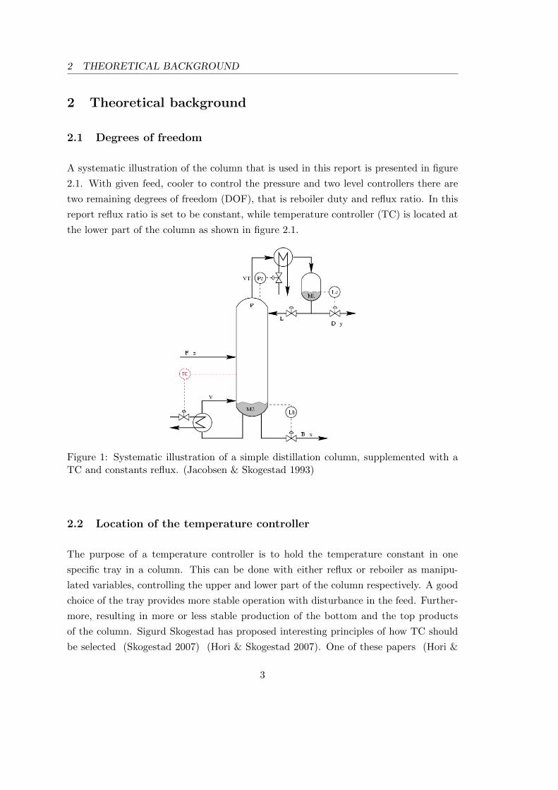
NTNU Fakultet for naturvitenskap og teknologi
Norges teknisk-naturvitenskapelige Institutt for kjemisk prosessteknologi
universitet
SPECIALIZATION PROJECT 2011
TKP 45
PROJECT TITLE:
Influence of feed rate and feed composition on a temperature
controller in a binary distillation column
By
Iakov Dolgov
Supervisor for the project: Sigurd Skogestad
Co-supervisor: Marius Støre Govatsmark (Statoil Kårstø)
Date: 16.12.2011
Abstract
Tuning of a temperature controller in a distillation column is very dependent on feed
rate, feed composition and in some cases composition of the products of the column.
Tight tuning done at high feed rate and minor content of light component in the feed
may result in unstable control at lower feed rate and major content of light component
in the feed. This project elaborates how oscillations caused by unstable control could
be avoided in a binary distillation column. The proposed methods are smooth tuning
of the controller and gain scheduling. The latter was found to be almost inevitable if
distillation column has large variation in feed rate. While a smooth global tuning is
found to be sufficient enough for variation in feed composition. Regarding the variation
of composition in product streams, the gain scheduling was found to be unnecessary if
set point in temperature controller is kept at some certain boundaries. MPC models at
different operation conditions were also presented in this report.
Acknowledgment
A big gratitude is directed to Sigurd Skogestad for sharing his model of distillation
column, but also for continuous help in preface and during the execution of the
simulation. Another big acknowledgment is directed to Marius Stre Govatsmark for his
encouraging and effective visits at NTNU during the semester and his e-mail support.
1) Reflux constraint ignored 2) Reflux constraint active
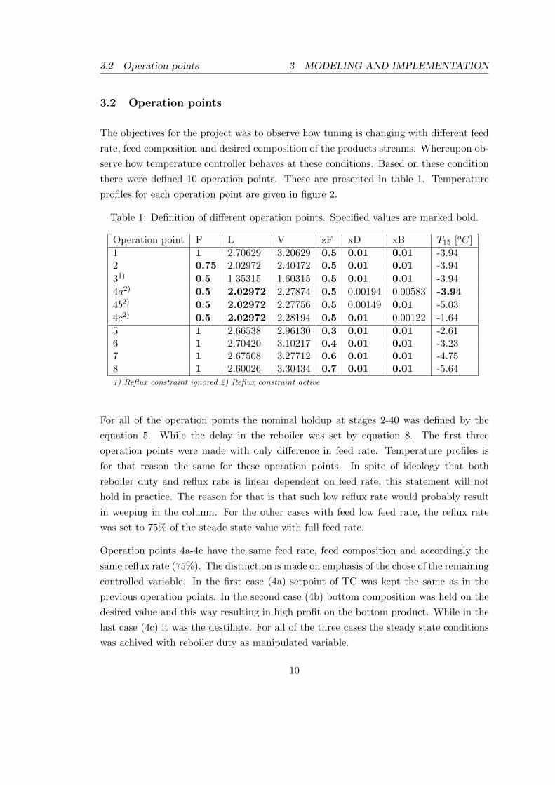
For all of the operation points the nominal holdup at stages 2-40 was defined by the
equation 5. While the delay in the reboiler was set by equation 8. The first three
operation points were made with only difference in feed rate. Temperature profiles is
for that reason the same for these operation points. In spite of ideology that both
reboiler duty and reflux rate is linear dependent on feed rate, this statement will not
hold in practice. The reason for that is that such low reflux rate would probably result
in weeping in the column. For the other cases with feed low feed rate, the reflux rate
was set to 75% of the steade state value with full feed rate.
Operation points 4a-4c have the same feed rate, feed composition and accordingly the
same reflux rate (75%). The distinction is made on emphasis of the chose of the remaining
controlled variable. In the first case (4a) setpoint of TC was kept the same as in the
previous operation points. In the second case (4b) bottom composition was held on the
desired value and this way resulting in high profit on the bottom product. While in the
last case (4c) it was the destillate. For all of the three cases the steady state conditions
was achived with reboiler duty as manipulated variable.
10
3 MODELING AND IMPLEMENTATION 3.2 Operation points
The remaining operation points (5-8) were created with consideration of the feed com-
position. The compositions of product streams are held at the desired values in all of
the cases. The steady state conditions were achieved with both reboiler duty and reflux
rate as manipulated variable for the product streams.
5 10 15 20 25 30 35 40
−11
−10
−9
−8
−7
−6
−5
−4
−3
−2
−1
Stage number
Tem
pera
ture
[oC
]
Operation point 1−3Operation point 4aOperation point 4bOperation point 4cOperation point 5Operation point 6Operation point 7Operation point 8Temperature controllers in operation points 1−4aTemperature controller in operation point 4bTemperature controller in operation point 4cTemperature controller in operation point 5Temperature controller in operation point 6Temperature controller in operation point 7Temperature controller in operation point 8
Figure 2: Temperature profiles at different operation points, with bottom to top enu-meration.
M-file code ”Starter All.m” can be used to run the simulation at different operation
points, both for tuning an open loop, but also to compare the tuning results with dis-
turbances in feed rate and feed composition. The description is added in the begging of
the file and is also giving in appendix D. For creation of MPC models the file
”starter All MPCmodels.m” can be used. Both files runs simulink file
”colas nonlin operation All.mdl” which is also given in in appendix E.
11
4 RESULTS
4 Results
4.1 Tuning results
Temperature controller was tuned at different operation points. In all cases the tun-
ing was done with equations 9 and 10, assuming pure integrating response and tuning
parameter (τc) equal to total delay (Θ). The results of tuning are presented in table 2
For consideration of gain scheduling it was found strong correlation between k′ ·Θ and
feed rate as well as k′ ·Θ and feed composition. This is presented in figure 3.
0.5 0.55 0.6 0.65 0.7 0.75 0.8 0.85 0.9 0.95 11
2
3
4
5
6
7
Feed rate (normalized)
Tun
ing
para
met
er: Θ
*k
Without constraint on minimum refluks valueWith constraint on minimum refluks value, operation point 4aWith constraint on minimum refluks value, operation point 4bWith constraint on minimum refluks value, operation point 4c
(a) Results of tuning at different feed rates
0.3 0.35 0.4 0.45 0.5 0.55 0.6 0.65
1.4
1.6
1.8
2
2.2
2.4
2.6
2.8
Fraction of light component in the feed
Tun
ing
para
met
er: Θ
*k
(b) Results of tuning at different feed composition
Figure 3: Correlation between k′ ·Θ and feed rate a), feed composition b).
As shown in figure 3 and more elaborated in appendix C the tuning parameters are
hard dependent on how the distillation column is operated. For instance, impurities in
the distillate or bottom product would reduce tuning significant. However, if set point
in temperature controller is held constant (operation point 4a), a linear correlation on
tunings parameters and feed rate is observed. The regression line is evaluated to be:
y = −5.42x+ 7.32 with gain scheduling factor of −5.42 as sketched in figure 4.
13
4.2 Simulation results 4 RESULTS
0.5 0.55 0.6 0.65 0.7 0.75 0.8 0.85 0.9 0.95 11
2
3
4
5
6
7
Feed rate (normalized)
Tun
ing
para
met
er: Θ
*k
Without constraint on minimum reflux valueOperation point 4a (active constraint on minimum reflux value)Operation point 4b (active constraint on minimum reflux value)Operation point 4c (active constraint on minimum reflux value)Fitted regression line: y=−5.42x+7.32
Figure 4: Correlation between k′ ·Θ and feed rate. Regression line is fitted to operationpoints with the same setpoint in TC.
4.2 Simulation results
The obtained tunings, that are showed in table 2 were implemented at different operation
points. The idea was to set tuning done at first operation point to the test at other
operation points and compare with new tuning at current operation point. A global
tuning was also suggested with characteristic smooth behavior.
The testing procedure was set to be disturbance at feed rate after 10 with magnitude of
0.1 and feed composition after 150 minutes with magnitude if 0.05. All of the simulations
are presented sequentially in appendix A. In this section operation point 3, 4b, 8 are
presented in figures 5- 7 respectively. All of the figure show temperature controller,
reboiler duty and impurity in distillate and bottom product with approximately the
same window as operator would see it.
14
4 RESULTS 4.2 Simulation results
0 50 100 150 200 250 300267
267.5
268
268.5
269
269.5
270
270.5
271
271.5
272
272.5
Time [min]
Tem
pera
ture
con
trol
ler
[o C]
SetpointController tuned at operation point 1
Controller retuned at current operation point Controller with recommended global tuning
(a) Temperature controller
0 50 100 150 200 250 3001.5
2
2.5
3
3.5
Time [min]
Reb
oile
r du
ty
Controller tuned at operation point 1
Controller retuned at current operation point Controller with recommended global tuning
(b) Reboiler
0 50 100 150 200 250 3000
0.005
0.01
0.015
0.02
0.025
0.03
0.035
Time [min]
Impu
rity
in to
p pr
oduc
t
Controller tuned at operation point 1
Controller retuned at current operation point Controller with recommended global tuning
(c) Impurity in top product
0 50 100 150 200 250 3000
0.005
0.01
0.015
0.02
0.025
0.03
0.035
Time [min]
Impu
rity
in b
otto
m p
rodu
ct
Controller tuned at operation point 1
Controller retuned at current operation point Controller with recommended global tuning
(d) Impurity in bottom product
Figure 5: Behavior of temperature controller a) at operation point 3 with disturbance infeed rate (dF=0.1) after 10 minutes and feed composition (dzF=-0.05) after 150 minutes.
15
4.2 Simulation results 4 RESULTS
0 50 100 150 200 250 300267
267.5
268
268.5
269
269.5
270
270.5
271
271.5
272
272.5
Time [min]
Tem
pera
ture
con
trol
ler
[o C]
SetpointController tuned at operation point 1
Controller retuned at current operation point Controller with recommended global tuning
(a) Temperature controller
0 50 100 150 200 250 3001.5
2
2.5
3
3.5
Time [min]
Reb
oile
r du
ty
Controller tuned at operation point 1
Controller retuned at current operation point Controller with recommended global tuning
(b) Reboiler
0 50 100 150 200 250 3000
0.005
0.01
0.015
0.02
0.025
0.03
0.035
Time [min]
Impu
rity
in to
p pr
oduc
t
Controller tuned at operation point 1
Controller retuned at current operation point Controller with recommended global tuning
(c) Impurity in top product
0 50 100 150 200 250 3000
0.005
0.01
0.015
0.02
0.025
0.03
0.035
Time [min]
Impu
rity
in b
otto
m p
rodu
ct
Controller tuned at operation point 1
Controller retuned at current operation point Controller with recommended global tuning
(d) Impurity in bottom product
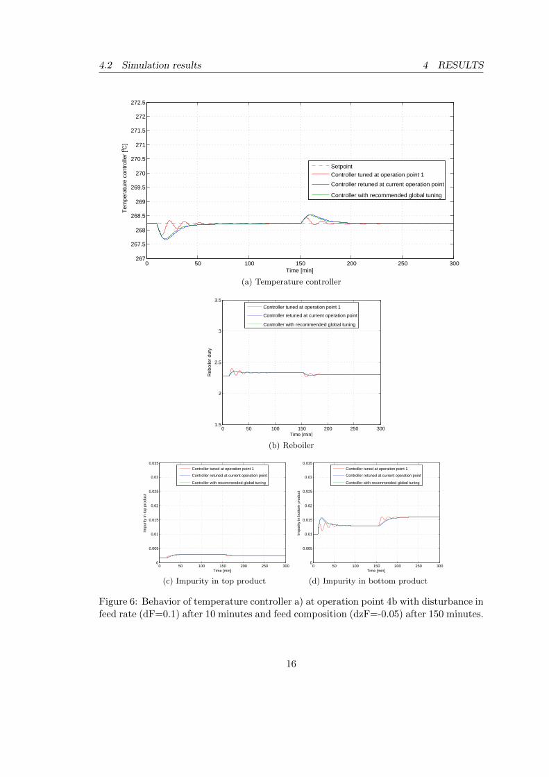
Figure 6: Behavior of temperature controller a) at operation point 4b with disturbance infeed rate (dF=0.1) after 10 minutes and feed composition (dzF=-0.05) after 150 minutes.
16
4 RESULTS 4.2 Simulation results
0 50 100 150 200 250 300267
267.5
268
268.5
269
269.5
270
270.5
271
271.5
272
272.5
Time [min]
Tem
pera
ture
con
trol
ler
[o C]
SetpointController tuned at operation point 1
Controller retuned at current operation point Controller with recommended global tuning
(a) Temperature controller
0 50 100 150 200 250 3001.5
2
2.5
3
3.5
Time [min]
Reb
oile
r du
ty
Controller tuned at operation point 1
Controller retuned at current operation point Controller with recommended global tuning
(b) Reboiler
0 50 100 150 200 250 3000
0.005
0.01
0.015
0.02
0.025
0.03
0.035
Time [min]
Impu
rity
in to
p pr
oduc
t
Controller tuned at operation point 1
Controller retuned at current operation point Controller with recommended global tuning
(c) Impurity in top product
0 50 100 150 200 250 3000
0.005
0.01
0.015
0.02
0.025
0.03
0.035
Time [min]
Impu
rity
in b
otto
m p
rodu
ct
Controller tuned at operation point 1
Controller retuned at current operation point Controller with recommended global tuning
(d) Impurity in bottom product
Figure 7: Behavior of temperature controller a) at operation point 8 with disturbance infeed rate (dF=0.1) after 10 minutes and feed composition (dzF=-0.05) after 150 minutes.
17
4.3 MPC models 4 RESULTS
4.3 MPC models
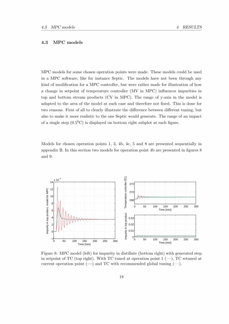
MPC models for some chosen operation points were made. These models could be used
in a MPC software, like for instance Septic. The models have not been through any
kind of modification for a MPC controller, but were rather made for illustration of how
a change in setpoint of temperature controller (MV in MPC) influences impurities in
top and bottom stream products (CV in MPC). The range of y-axis in the model is
adapted to the area of the model at each case and therefore not fixed. This is done for
two reasons. First of all to clearly illustrate the difference between different tuning, but
also to make it more realistic to the one Septic would generate. The range of an impact
of a single step (0.50C) is displayed on bottom right subplot at each figure.
Models for chosen operation points 1, 3, 4b, 4c, 5 and 8 are presented sequentially in
appendix B. In this section two models for operation point 4b are presented in figures 8
and 9.
0 50 100 150 200 250 300−2
0
2
4
6
8
10
12
14x 10
−4
Time [min]
Impu
rity
in to
p pr
oduc
t, m
odel
for
MP
C
0 50 100 150 200 250 300
268
270
272
Time [min]
Tem
pera
ture
con
trol
ler
[o C]
0 50 100 150 200 250 3000
0.01
0.02
0.03
Time [min]
Impu
rity
in to
p pr
oduc
t
Figure 8: MPC model (left) for impurity in distillate (bottom right) with generated stepin setpoint of TC (top right). With TC tuned at operation point 1 (—), TC retuned atcurrent operation point (—) and TC with recommended global tuning (—).
18
4 RESULTS 4.3 MPC models
0 50 100 150 200 250 300−10
−8
−6
−4
−2
0
2x 10
−3
Time [min]
Impu
rity
in b
otto
m p
rodu
ct, m
odel
for
MP
C
0 50 100 150 200 250 300
268
270
272
Time [min]
Tem
pera
ture
con
trol
ler
[o C]
0 50 100 150 200 250 3000
0.01
0.02
0.03
Time [min]Im
purit
y in
bot
tom
pro
duct
Figure 9: MPC model (left) for impurity in bottom product (bottom right) with gener-ated step in setpoint of TC (top right). With TC tuned at operation point 1 (—), TCretuned at current operation point (—) and TC with recommended global tuning (—).
19
5 DISCUSSION
5 Discussion
In equation 15 it was found that controller gain is non linear correlated to reboiler duty.
In this report the reference values of reboiler duty, delay in the reboiler and liquid tray
holdup were used from the first operation point and applied in calculations of k′ ·Θ with
equation 15. The values were then compared with values from process (table 3).
The results show that all of the approximation done in section 2.3 can be excepted at
certain operation conditions. Calculated and process values at for example operation
points 1-3, with only differences in feed rate, follows the same trend. However, the trend
is not followed at operation points 5-8. The reason for that could be approximation done
in equations 13- 14, since feed composition influences composition at each stage, what
is clearly observed in temperature profiles in figure 2.
Regarding operation points 4a-4c it is observed that process values changes, but the
calculated values remains almost the same, due to the fact that they are dependent only
at reboiler duty, which has almost no variation (table 1). The variation of the process
values can be explained by investigate these operation points one by one.
When feed rate drops significant, constraint on minimum reflux would be reached (75%)
and further operation needs to be specified by which product stream should be given up
to control. In that case operator of the column would have three alternatives:
1. Give up composition control in both product streams and rather control the tem-
perature in the column (operation point 4a). In this case both product stream
would be overpurified, but temperature would be kept at the same setpoint.
2. Give up composition control in distillate product and rather prioritize control of the
bottom stream (operation point 4b). This would result in increase of purification
in the distillate stream. The choice could be preferred if the price of the light
component is smaller then the heavy component.
3. Give up composition control in bottom product and rather prioritize control of
distillate (operation point 4c). This would result in increase of purification in the
bottom stream. The choice could be preferred if the price of the heavy component
is smaller then the light component.
In the case with binary mixture with n-butane and isobutane. The latter one is expected
to be more expensive and should therefore be produced at largest possible scale. If the
20
5 DISCUSSION
feed rate is set, the best solution is to keep impurity at highest profitable value and
overpurify the other stream. Since isobutane is the light component in the mixture,
operation point 4c is the most profitable from these three operations.
From the control point of view operation point 4c is the one with smallest process gain
(table 2), but a small increase of reboiler duty has a tremendous effect on top product
at this operation point. The explanation for that is lying in the fact that temperature
controller at this point is far from nominal value. A small disturbance in the feed would
therefore pollute the product stream far over the desired level, making the product hard
to sell. However, operation points 4a and 4b does not have this behavior. One suggestion
for the best operation point could be a compromise between operation point 4b and
4c. This could be done by adding constrains in the temperature controller. On the
other hand, it is important to state the fact that reflux was not used as a manipulated
variable in simulations with disturbances and problem with the tremendous effect on
the top product would be by far from so tremendous if reflux would be used to control
composition in distillate by for example MPC, which can handles reflux constraint in a
proper way.
Nevertheless if the prices of products are expected to be varying and changes of active
constrains are demanded. The set point of TC i forced to be changing. An option in
such case could be an individual gain schedule. However, this can be avoided if setpoint
of TC is designed to have only small variations, i.e. add constraints as explained above.
Even though this will not result in maximum utilization of the valuable product, the
control structure would be much simpler.
Regarding simulation results, it was obvious that tuning done at first operation point
gave oscillatory behavior at lower feed rates. A global tuning was therefore suggested.
The tuning had smooth behavior in all of the operation points, but could be considered
too slow at high feed rate and high content of light component in the feed. Consequently,
a linear gain scheduling with consideration of feed rate was suggested. The factor was
found to be 5.42 and was based on the fact that temperature controller would be kept
at the same value at different feed rates. Even though in theory it was found non linear
relation between reboiler duty and tuning parameters, the empirically obtained linear
simplification is suitable when constrain on minimum reflux is taken into consideration.
Gain scheduling with consideration of feed composition was not evaluated. On of the
reasons for that is that tuning from the first operation point was not found to have
oscillatory behavior at these operation points. Recommendation for further work could
21
5 DISCUSSION
be to see if this is the case with other models then column A.
Later in the report there were found MPC models for some interesting operation point.
Some strong oscillations were noticed with controller tuning from the first operation
point. These were observed, as expected, in operation points 3 and 4b. Even Septic,
which is a good MPC software would have problems controlling a process with these
(red) models. Regarding the global tuning, in most operations it had a similar model as
retuned controller and Septic would probably not have problems.
The alarming fact with developed MPC models appeared when gain of one model de-
veloped at one operation point was mutually compared with another model developed
at different operation point. Put another way, if models that were developed at one op-
eration points would be used at other feed rates and feed compositions, the MPC would
probably have total different behavior. The vast variation of the gain is observed be-
tween operation points 3 and 4c regarding the models for distillate and operation points
4b and 5 regarding the models for bottom product. The variation can be summarized
with following enumeration:
• If the CV is initially overpurified, the models would have small gain.
• If the CV is kept at the constrain, but the other product stream is overpurified,
the models would have abundant large gain.
• An increase of feed rate with same composition in product streams and set point
for TC does not result in significant change of the model.
• An increase of light component content in the feed stream results in gain reduction
of the model. Equivalently, low content of light component results in gain increase
of the model.
The models were made for illustration of how a change in setpoint of temperature con-
troller in influences impurities distillate and bottom stream products. The models have
not been through any kind of modification for a MPC controller, and should not be
implemented directly in a MPC software. Recommendation for further work could be to
evaluate the behavior of MPC at different operation points and different MPC models.
22
6 CONCLUSION
6 Conclusion
In this project behavior of a single temperature controller in a distillation was investi-
gated. Column A was used as a model for distillation column with a simple relationship
between composition and temperature at each stage. Several operation points were de-
fined, with variation in feed rate, feed composition and composition in product streams.
Tuning of the temperature controller was done at initial operation conditions and eval-
uated at other operation points. The result was that initial tunings had oscillatory
characteristics when the feed rate was reduced significantly. It was therefore suggested
linear gain scheduling with magnitude of 5.42. It was also suggested that global tuning
for the controller could be used at various feed compositions. Regarding variation of
composition in product streams, the tuning at current feed rate was found to be suitable
if set point in temperature controller is kept at some certain boundaries. Considering
supervisory control layer, it as found that the developed models at certain operation
conditions should be evaluated before implementation.
Trondheim 16.desember 2011
—————————–
Iakov Dolgov
23
REFERENCES REFERENCES
References
Halvorsen, I. J., Skogestad, S., Morud, J. C. & Alstad, V. (2003), ‘Optimal selection of
controlled variables’, Ind. Eng. Chem. Res 42, 3273–3284.
Hori, E. S. & Skogestad, S. (2007), ‘Selection of control structure and temperature
location for two-product distillation columns’, Trans IChemE 85(A3), 293–306.
Jang, J., Annaswamy, A. M. & Lavretsky, E. (2008), Adaptive control of time-varying
systems with gain-scheduling, in ‘American Control Conference’.
Luyben, W. L. (2005), ‘Effect of feed composition on the selection of control structures
for high-purity binary distillation’, Ind. Eng. Chem. Res 44, 7800–7813.
Skogestad, S. (2007), ‘The dos and dont-ts of distillation column control’, Trans IChemE
85(A1), 13–23.
Skogestad, S. & Grimholt, C. (2011), ‘The simc method for smooth pid controller tuning’.
Skogestad, S. & Morari, M. (1988), ‘Understanding the dynamic behavior of distillation
columns’, Ind . Eng. Chem. Res 27, 1859.
Wittgens, B. & Skogestad, S. (2000), ‘Evaluation of dynamic models of distillation
columns with emphasis on the initial response’, MIC 21, 83–103.
24
A SIMULATION
Appendices
A Simulation
25
A.1 Operation point 1 A SIMULATION
A.1 Operation point 1
0 50 100 150 200 250 300267
267.5
268
268.5
269
269.5
270
270.5
271
271.5
272
272.5
Time [min]
Tem
pera
ture
con
trol
ler
[o C]
SetpointController tuned at operation point 1
Controller retuned at current operation point Controller with recommended global tuning
(a) Temperature controller
0 50 100 150 200 250 3001.5
2
2.5
3
3.5
Time [min]
Reb
oile
r du
ty
Controller tuned at operation point 1
Controller retuned at current operation point Controller with recommended global tuning
(b) Reboiler
0 50 100 150 200 250 3000
0.005
0.01
0.015
0.02
0.025
0.03
0.035
Time [min]
Impu
rity
in to
p pr
oduc
t
Controller tuned at operation point 1
Controller retuned at current operation point Controller with recommended global tuning
(c) Impurity in top product
0 50 100 150 200 250 3000
0.005
0.01
0.015
0.02
0.025
0.03
0.035
Time [min]
Impu
rity
in b
otto
m p
rodu
ct
Controller tuned at operation point 1
Controller retuned at current operation point Controller with recommended global tuning
(d) Impurity in bottom product
Figure 10: Behavior of temperature controller a) at operation point 1 with disturbance infeed rate (dF=0.1) after 10 minutes and feed composition (dzF=-0.05) after 150 minutes.Reboiler duty b) was used as input for the controller resulting in impurity changes inrespectively top c) and bottom product streams d).
26
A SIMULATION A.2 Operation point 2
A.2 Operation point 2
0 50 100 150 200 250 300267
267.5
268
268.5
269
269.5
270
270.5
271
271.5
272
272.5
Time [min]
Tem
pera
ture
con
trol
ler
[o C]
SetpointController tuned at operation point 1
Controller retuned at current operation point Controller with recommended global tuning
(a) Temperature controller
0 50 100 150 200 250 3001.5
2
2.5
3
3.5
Time [min]
Reb
oile
r du
ty
Controller tuned at operation point 1
Controller retuned at current operation point Controller with recommended global tuning
(b) Reboiler
0 50 100 150 200 250 3000
0.005
0.01
0.015
0.02
0.025
0.03
0.035
Time [min]
Impu
rity
in to
p pr
oduc
t
Controller tuned at operation point 1
Controller retuned at current operation point Controller with recommended global tuning
(c) Impurity in top product
0 50 100 150 200 250 3000
0.005
0.01
0.015
0.02
0.025
0.03
0.035
Time [min]
Impu
rity
in b
otto
m p
rodu
ct
Controller tuned at operation point 1
Controller retuned at current operation point Controller with recommended global tuning
(d) Impurity in bottom product
Figure 11: Behavior of temperature controller a) at operation point 2 with disturbance infeed rate (dF=0.1) after 10 minutes and feed composition (dzF=-0.05) after 150 minutes.Reboiler duty b) was used as input for the controller resulting in impurity changes inrespectively top c) and bottom product streams d).
27
A.3 Operation point 3 A SIMULATION
A.3 Operation point 3
0 50 100 150 200 250 300267
267.5
268
268.5
269
269.5
270
270.5
271
271.5
272
272.5
Time [min]
Tem
pera
ture
con
trol
ler
[o C]
SetpointController tuned at operation point 1
Controller retuned at current operation point Controller with recommended global tuning
(a) Temperature controller
0 50 100 150 200 250 3001.5
2
2.5
3
3.5
Time [min]
Reb
oile
r du
ty
Controller tuned at operation point 1
Controller retuned at current operation point Controller with recommended global tuning
(b) Reboiler
0 50 100 150 200 250 3000
0.005
0.01
0.015
0.02
0.025
0.03
0.035
Time [min]
Impu
rity
in to
p pr
oduc
t
Controller tuned at operation point 1
Controller retuned at current operation point Controller with recommended global tuning
(c) Impurity in top product
0 50 100 150 200 250 3000
0.005
0.01
0.015
0.02
0.025
0.03
0.035
Time [min]
Impu
rity
in b
otto
m p
rodu
ct
Controller tuned at operation point 1
Controller retuned at current operation point Controller with recommended global tuning
(d) Impurity in bottom product
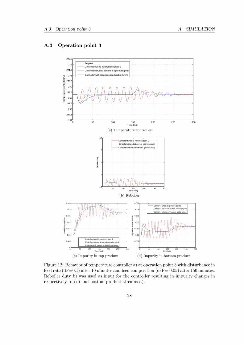
Figure 12: Behavior of temperature controller a) at operation point 3 with disturbance infeed rate (dF=0.1) after 10 minutes and feed composition (dzF=-0.05) after 150 minutes.Reboiler duty b) was used as input for the controller resulting in impurity changes inrespectively top c) and bottom product streams d).
28
A SIMULATION A.4 Operation point 4a
A.4 Operation point 4a
0 50 100 150 200 250 300267
267.5
268
268.5
269
269.5
270
270.5
271
271.5
272
272.5
Time [min]
Tem
pera
ture
con
trol
ler
[o C]
SetpointController tuned at operation point 1
Controller retuned at current operation point Controller with recommended global tuning
(a) Temperature controller
0 50 100 150 200 250 3001.5
2
2.5
3
3.5
Time [min]
Reb
oile
r du
ty
Controller tuned at operation point 1
Controller retuned at current operation point Controller with recommended global tuning
(b) Reboiler
0 50 100 150 200 250 3000
0.005
0.01
0.015
0.02
0.025
0.03
0.035
Time [min]
Impu
rity
in to
p pr
oduc
t
Controller tuned at operation point 1
Controller retuned at current operation point Controller with recommended global tuning
(c) Impurity in top product
0 50 100 150 200 250 3000
0.005
0.01
0.015
0.02
0.025
0.03
0.035
Time [min]
Impu
rity
in b
otto
m p
rodu
ct
Controller tuned at operation point 1
Controller retuned at current operation point Controller with recommended global tuning
(d) Impurity in bottom product
Figure 13: Behavior of temperature controller a) at operation point 4a with disturbancein feed rate (dF=0.1) after 10 minutes and feed composition (dzF=-0.05) after 150minutes. Reboiler duty b) was used as input for the controller resulting in impuritychanges in respectively top c) and bottom product streams d).
29
A.5 Operation point 4b A SIMULATION
A.5 Operation point 4b
0 50 100 150 200 250 300267
267.5
268
268.5
269
269.5
270
270.5
271
271.5
272
272.5
Time [min]
Tem
pera
ture
con
trol
ler
[o C]
SetpointController tuned at operation point 1
Controller retuned at current operation point Controller with recommended global tuning
(a) Temperature controller
0 50 100 150 200 250 3001.5
2
2.5
3
3.5
Time [min]
Reb
oile
r du
ty
Controller tuned at operation point 1
Controller retuned at current operation point Controller with recommended global tuning
(b) Reboiler
0 50 100 150 200 250 3000
0.005
0.01
0.015
0.02
0.025
0.03
0.035
Time [min]
Impu
rity
in to
p pr
oduc
t
Controller tuned at operation point 1
Controller retuned at current operation point Controller with recommended global tuning
(c) Impurity in top product
0 50 100 150 200 250 3000
0.005
0.01
0.015
0.02
0.025
0.03
0.035
Time [min]
Impu
rity
in b
otto
m p
rodu
ct
Controller tuned at operation point 1
Controller retuned at current operation point Controller with recommended global tuning
(d) Impurity in bottom product
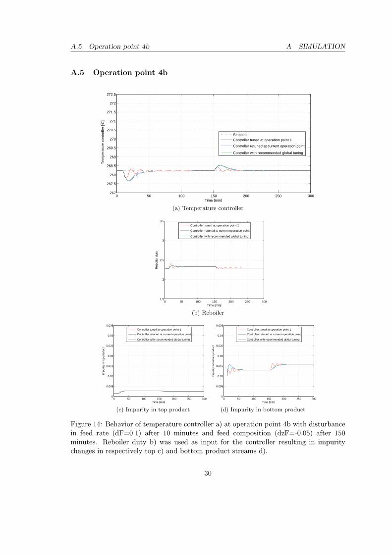
Figure 14: Behavior of temperature controller a) at operation point 4b with disturbancein feed rate (dF=0.1) after 10 minutes and feed composition (dzF=-0.05) after 150minutes. Reboiler duty b) was used as input for the controller resulting in impuritychanges in respectively top c) and bottom product streams d).
30
A SIMULATION A.6 Operation point 4c
A.6 Operation point 4c
0 50 100 150 200 250 300267
267.5
268
268.5
269
269.5
270
270.5
271
271.5
272
272.5
Time [min]
Tem
pera
ture
con
trol
ler
[o C]
SetpointController tuned at operation point 1
Controller retuned at current operation point Controller with recommended global tuning
(a) Temperature controller
0 50 100 150 200 250 3001.5
2
2.5
3
3.5
Time [min]
Reb
oile
r du
ty
Controller tuned at operation point 1
Controller retuned at current operation point Controller with recommended global tuning
(b) Reboiler
0 50 100 150 200 250 3000
0.005
0.01
0.015
0.02
0.025
0.03
0.035
Time [min]
Impu
rity
in to
p pr
oduc
t
Controller tuned at operation point 1
Controller retuned at current operation point Controller with recommended global tuning
(c) Impurity in top product
0 50 100 150 200 250 3000
0.005
0.01
0.015
0.02
0.025
0.03
0.035
Time [min]
Impu
rity
in b
otto
m p
rodu
ct
Controller tuned at operation point 1
Controller retuned at current operation point Controller with recommended global tuning
(d) Impurity in bottom product
Figure 15: Behavior of temperature controller a) at operation point 4c with disturbancein feed rate (dF=0.1) after 10 minutes and feed composition (dzF=-0.05) after 150minutes. Reboiler duty b) was used as input for the controller resulting in impuritychanges in respectively top c) and bottom product streams d).
31
A.7 Operation point 5 A SIMULATION
A.7 Operation point 5
0 50 100 150 200 250 300267
267.5
268
268.5
269
269.5
270
270.5
271
271.5
272
272.5
Time [min]
Tem
pera
ture
con
trol
ler
[o C]
SetpointController tuned at operation point 1
Controller retuned at current operation point Controller with recommended global tuning
(a) Temperature controller
0 50 100 150 200 250 3001.5
2
2.5
3
3.5
Time [min]
Reb
oile
r du
ty
Controller tuned at operation point 1
Controller retuned at current operation point Controller with recommended global tuning
(b) Reboiler
0 50 100 150 200 250 3000
0.005
0.01
0.015
0.02
0.025
0.03
0.035
Time [min]
Impu
rity
in to
p pr
oduc
t
Controller tuned at operation point 1
Controller retuned at current operation point Controller with recommended global tuning
(c) Impurity in top product
0 50 100 150 200 250 3000
0.005
0.01
0.015
0.02
0.025
0.03
0.035
Time [min]
Impu
rity
in b
otto
m p
rodu
ct
Controller tuned at operation point 1
Controller retuned at current operation point Controller with recommended global tuning
(d) Impurity in bottom product
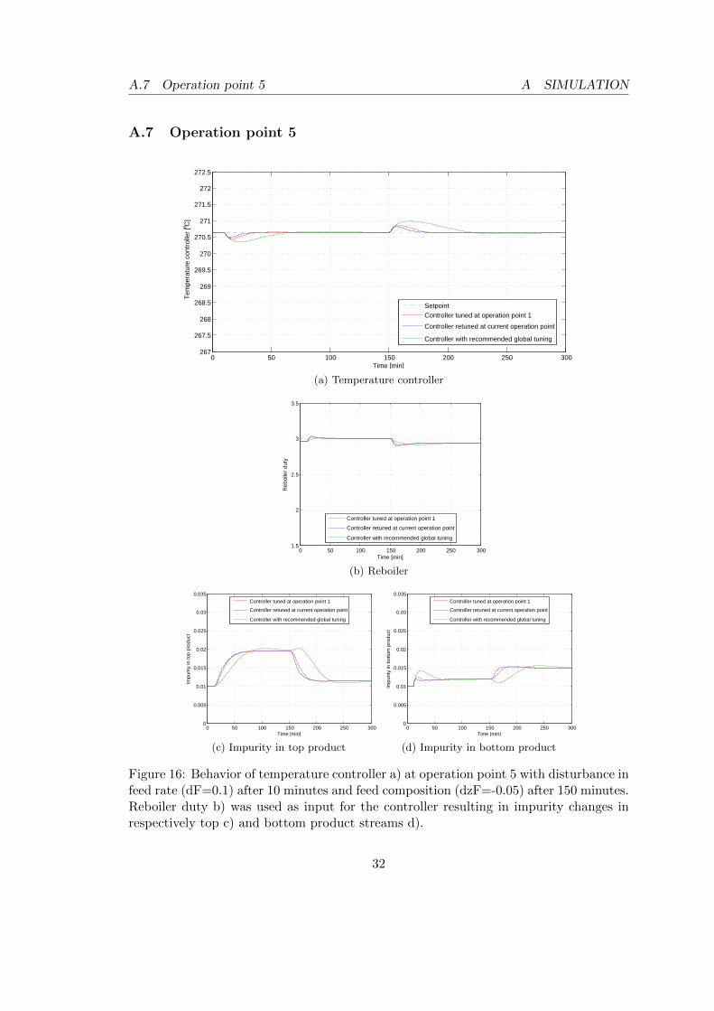
Figure 16: Behavior of temperature controller a) at operation point 5 with disturbance infeed rate (dF=0.1) after 10 minutes and feed composition (dzF=-0.05) after 150 minutes.Reboiler duty b) was used as input for the controller resulting in impurity changes inrespectively top c) and bottom product streams d).
32
A SIMULATION A.8 Operation point 6
A.8 Operation point 6
0 50 100 150 200 250 300267
267.5
268
268.5
269
269.5
270
270.5
271
271.5
272
272.5
Time [min]
Tem
pera
ture
con
trol
ler
[o C]
SetpointController tuned at operation point 1
Controller retuned at current operation point Controller with recommended global tuning
(a) Temperature controller
0 50 100 150 200 250 3001.5
2
2.5
3
3.5
Time [min]
Reb
oile
r du
ty
Controller tuned at operation point 1
Controller retuned at current operation point Controller with recommended global tuning
(b) Reboiler
0 50 100 150 200 250 3000
0.005
0.01
0.015
0.02
0.025
0.03
0.035
Time [min]
Impu
rity
in to
p pr
oduc
t
Controller tuned at operation point 1
Controller retuned at current operation point Controller with recommended global tuning
(c) Impurity in top product
0 50 100 150 200 250 3000
0.005
0.01
0.015
0.02
0.025
0.03
0.035
Time [min]
Impu
rity
in b
otto
m p
rodu
ct
Controller tuned at operation point 1
Controller retuned at current operation point Controller with recommended global tuning
(d) Impurity in bottom product
Figure 17: Behavior of temperature controller a) at operation point 6 with disturbance infeed rate (dF=0.1) after 10 minutes and feed composition (dzF=-0.05) after 150 minutes.Reboiler duty b) was used as input for the controller resulting in impurity changes inrespectively top c) and bottom product streams d).
33
A.9 Operation point 7 A SIMULATION
A.9 Operation point 7
0 50 100 150 200 250 300267
267.5
268
268.5
269
269.5
270
270.5
271
271.5
272
272.5
Time [min]
Tem
pera
ture
con
trol
ler
[o C]
SetpointController tuned at operation point 1
Controller retuned at current operation point Controller with recommended global tuning
(a) Temperature controller
0 50 100 150 200 250 3001.5
2
2.5
3
3.5
Time [min]
Reb
oile
r du
ty
Controller tuned at operation point 1
Controller retuned at current operation point Controller with recommended global tuning
(b) Reboiler
0 50 100 150 200 250 3000
0.005
0.01
0.015
0.02
0.025
0.03
0.035
Time [min]
Impu
rity
in to
p pr
oduc
t
Controller tuned at operation point 1
Controller retuned at current operation point Controller with recommended global tuning
(c) Impurity in top product
0 50 100 150 200 250 3000
0.005
0.01
0.015
0.02
0.025
0.03
0.035
Time [min]
Impu
rity
in b
otto
m p
rodu
ct
Controller tuned at operation point 1
Controller retuned at current operation point Controller with recommended global tuning
(d) Impurity in bottom product
Figure 18: Behavior of temperature controller a) at operation point 7 with disturbance infeed rate (dF=0.1) after 10 minutes and feed composition (dzF=-0.05) after 150 minutes.Reboiler duty b) was used as input for the controller resulting in impurity changes inrespectively top c) and bottom product streams d).
34
A SIMULATION A.10 Operation point 8
A.10 Operation point 8
0 50 100 150 200 250 300267
267.5
268
268.5
269
269.5
270
270.5
271
271.5
272
272.5
Time [min]
Tem
pera
ture
con
trol
ler
[o C]
SetpointController tuned at operation point 1
Controller retuned at current operation point Controller with recommended global tuning
(a) Temperature controller
0 50 100 150 200 250 3001.5
2
2.5
3
3.5
Time [min]
Reb
oile
r du
ty
Controller tuned at operation point 1
Controller retuned at current operation point Controller with recommended global tuning
(b) Reboiler
0 50 100 150 200 250 3000
0.005
0.01
0.015
0.02
0.025
0.03
0.035
Time [min]
Impu
rity
in to
p pr
oduc
t
Controller tuned at operation point 1
Controller retuned at current operation point Controller with recommended global tuning
(c) Impurity in top product
0 50 100 150 200 250 3000
0.005
0.01
0.015
0.02
0.025
0.03
0.035
Time [min]
Impu
rity
in b
otto
m p
rodu
ct
Controller tuned at operation point 1
Controller retuned at current operation point Controller with recommended global tuning
(d) Impurity in bottom product
Figure 19: Behavior of temperature controller a) at operation point 8 with disturbance infeed rate (dF=0.1) after 10 minutes and feed composition (dzF=-0.05) after 150 minutes.Reboiler duty b) was used as input for the controller resulting in impurity changes inrespectively top c) and bottom product streams d).
35
B MODELS FOR MPC
B Models for MPC
B.1 Operation point 1
0 50 100 150 200 250 300−1
0
1
2
3
4
5
6
7x 10
−3
Time [min]
Impu
rity
in to
p pr
oduc
t, m
odel
for
MP
C
0 50 100 150 200 250 300
268
270
272
Time [min]Tem
pera
ture
con
trol
ler
[o C]
0 50 100 150 200 250 3000
0.01
0.02
0.03
Time [min]
Impu
rity
in to
p pr
oduc
t
Figure 20: MPC model (left) for impurity in distillate (bottom right) with generatedstep in setpoint of TC (top right). With TC tuned at operation point 1 (—), TC retunedat current operation point (—) and TC with recommended global tuning (—).
0 50 100 150 200 250 300−7
−6
−5
−4
−3
−2
−1
0
1x 10
−3
Time [min]
Impu
rity
in b
otto
m p
rodu
ct, m
odel
for
MP
C
0 50 100 150 200 250 300
268
270
272
Time [min]
Tem
pera
ture
con
trol
ler
[o C]
0 50 100 150 200 250 3000
0.01
0.02
0.03
Time [min]
Impu
rity
in b
otto
m p
rodu
ct
Figure 21: MPC model (left) for impurity in bottom product (bottom right) with gen-erated step in setpoint of TC (top right). With TC tuned at operation point 1 (—), TCretuned at current operation point (—) and TC with recommended global tuning (—).
36
B MODELS FOR MPC B.2 Operation point 3
B.2 Operation point 3
0 50 100 150 200 250 300−0.01
0
0.01
0.02
0.03
0.04
0.05
0.06
Time [min]
Impu
rity
in to
p pr
oduc
t, m
odel
for
MP
C
0 50 100 150 200 250 300
268
270
272
Time [min]
Tem
pera
ture
con
trol
ler
[o C]
0 50 100 150 200 250 3000
0.01
0.02
0.03
Time [min]
Impu
rity
in to
p pr
oduc
t
Figure 22: MPC model (left) for impurity in distillate (bottom right) with generatedstep in setpoint of TC (top right). With TC tuned at operation point 1 (—), TC retunedat current operation point (—) and TC with recommended global tuning (—).
0 50 100 150 200 250 300−0.02
−0.01
0
0.01
0.02
0.03
0.04
0.05
Time [min]
Impu
rity
in b
otto
m p
rodu
ct, m
odel
for
MP
C
0 50 100 150 200 250 300
268
270
272
Time [min]
Tem
pera
ture
con
trol
ler
[o C]
0 50 100 150 200 250 3000
0.01
0.02
0.03
Time [min]
Impu
rity
in b
otto
m p
rodu
ct
Figure 23: MPC model (left) for impurity in bottom product (bottom right) with gen-erated step in setpoint of TC (top right). With TC tuned at operation point 1 (—), TCretuned at current operation point (—) and TC with recommended global tuning (—).
37
B.3 Operation point 4b B MODELS FOR MPC
B.3 Operation point 4b
0 50 100 150 200 250 300−2
0
2
4
6
8
10
12
14x 10
−4
Time [min]
Impu
rity
in to
p pr
oduc
t, m
odel
for
MP
C
0 50 100 150 200 250 300
268
270
272
Time [min]
Tem
pera
ture
con
trol
ler
[o C]
0 50 100 150 200 250 3000
0.01
0.02
0.03
Time [min]
Impu
rity
in to
p pr
oduc
t
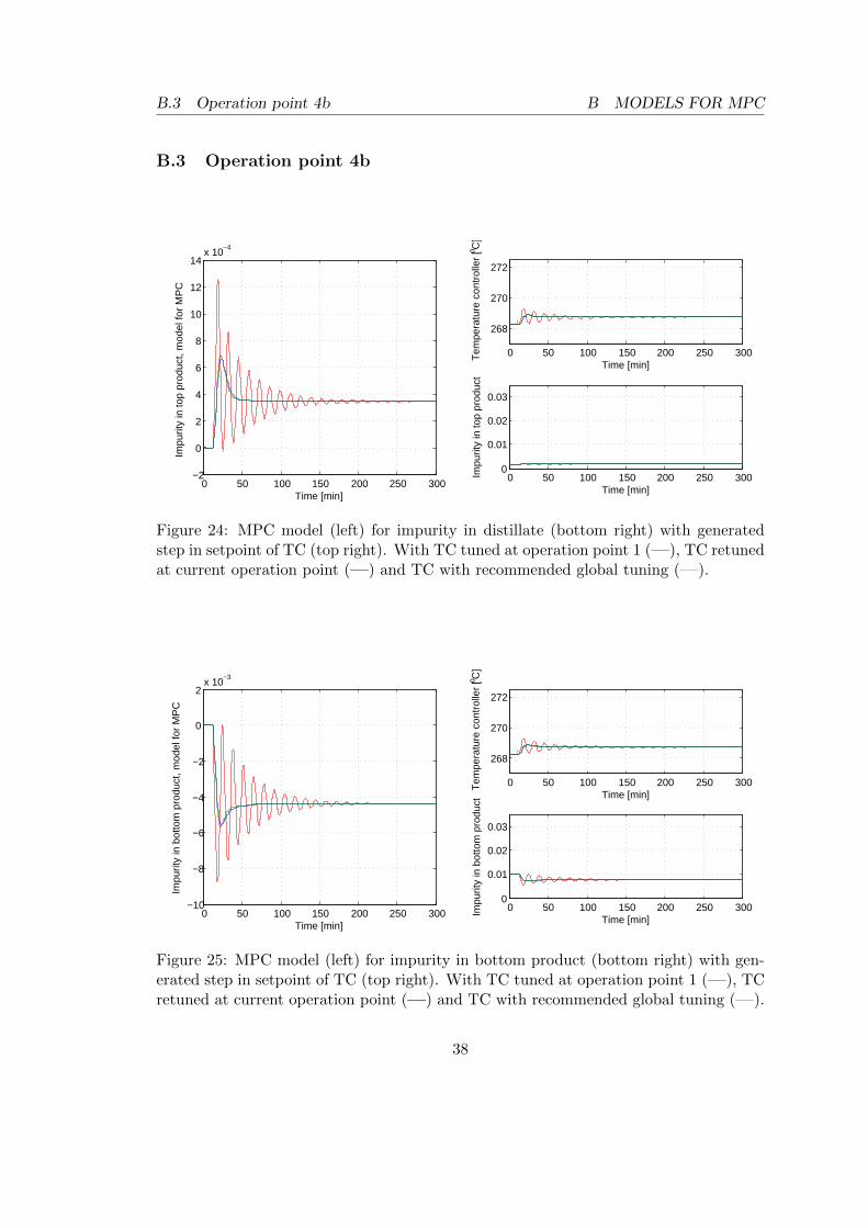
Figure 24: MPC model (left) for impurity in distillate (bottom right) with generatedstep in setpoint of TC (top right). With TC tuned at operation point 1 (—), TC retunedat current operation point (—) and TC with recommended global tuning (—).
0 50 100 150 200 250 300−10
−8
−6
−4
−2
0
2x 10
−3
Time [min]
Impu
rity
in b
otto
m p
rodu
ct, m
odel
for
MP
C
0 50 100 150 200 250 300
268
270
272
Time [min]
Tem
pera
ture
con
trol
ler
[o C]
0 50 100 150 200 250 3000
0.01
0.02
0.03
Time [min]
Impu
rity
in b
otto
m p
rodu
ct
Figure 25: MPC model (left) for impurity in bottom product (bottom right) with gen-erated step in setpoint of TC (top right). With TC tuned at operation point 1 (—), TCretuned at current operation point (—) and TC with recommended global tuning (—).
38
B MODELS FOR MPC B.4 Operation point 4c
B.4 Operation point 4c
0 50 100 150 200 250 3000
0.05
0.1
0.15
0.2
0.25
Time [min]
Impu
rity
in to
p pr
oduc
t, m
odel
for
MP
C
0 50 100 150 200 250 300
268
270
272
Time [min]
Tem
pera
ture
con
trol
ler
[o C]
0 50 100 150 200 250 3000
0.01
0.02
0.03
Time [min]
Impu
rity
in to
p pr
oduc
t
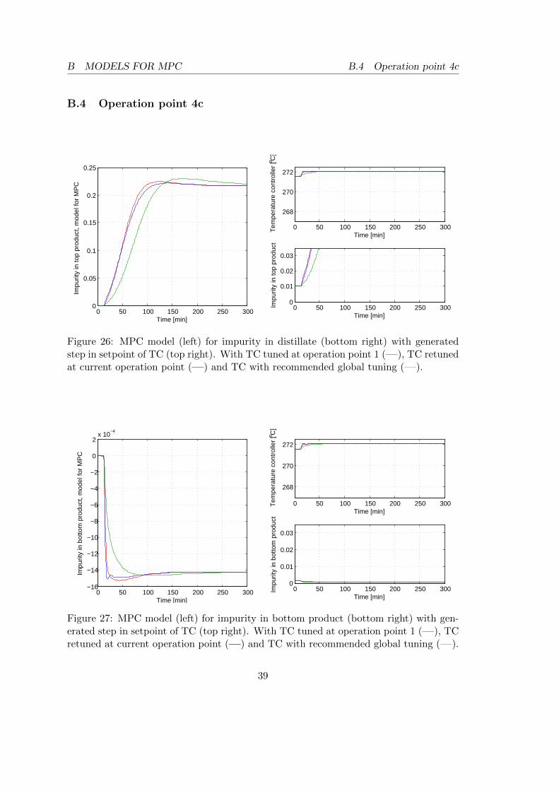
Figure 26: MPC model (left) for impurity in distillate (bottom right) with generatedstep in setpoint of TC (top right). With TC tuned at operation point 1 (—), TC retunedat current operation point (—) and TC with recommended global tuning (—).
0 50 100 150 200 250 300−16
−14
−12
−10
−8
−6
−4
−2
0
2x 10
−4
Time [min]
Impu
rity
in b
otto
m p
rodu
ct, m
odel
for
MP
C
0 50 100 150 200 250 300
268
270
272
Time [min]
Tem
pera
ture
con
trol
ler
[o C]
0 50 100 150 200 250 3000
0.01
0.02
0.03
Time [min]
Impu
rity
in b
otto
m p
rodu
ct
Figure 27: MPC model (left) for impurity in bottom product (bottom right) with gen-erated step in setpoint of TC (top right). With TC tuned at operation point 1 (—), TCretuned at current operation point (—) and TC with recommended global tuning (—).
39
B.5 Operation point 5 B MODELS FOR MPC
B.5 Operation point 5
0 50 100 150 200 250 300−0.005
0
0.005
0.01
0.015
0.02
0.025
0.03
Time [min]
Impu
rity
in to
p pr
oduc
t, m
odel
for
MP
C
0 50 100 150 200 250 300
268
270
272
Time [min]
Tem
pera
ture
con
trol
ler
[o C]
0 50 100 150 200 250 3000
0.01
0.02
0.03
Time [min]
Impu
rity
in to
p pr
oduc
t
Figure 28: MPC model (left) for impurity in distillate (bottom right) with generatedstep in setpoint of TC (top right). With TC tuned at operation point 1 (—), TC retunedat current operation point (—) and TC with recommended global tuning (—).
0 50 100 150 200 250 300−10
−8
−6
−4
−2
0
2x 10
−3
Time [min]
Impu
rity
in b
otto
m p
rodu
ct, m
odel
for
MP
C
0 50 100 150 200 250 300
268
270
272
Time [min]
Tem
pera
ture
con
trol
ler
[o C]
0 50 100 150 200 250 3000
0.01
0.02
0.03
Time [min]
Impu
rity
in b
otto
m p
rodu
ct
Figure 29: MPC model (left) for impurity in bottom product (bottom right) with gen-erated step in setpoint of TC (top right). With TC tuned at operation point 1 (—), TCretuned at current operation point (—) and TC with recommended global tuning (—).
40
B MODELS FOR MPC B.6 Operation point 8
B.6 Operation point 8
0 50 100 150 200 250 3000
0.5
1
1.5
2
2.5
3
3.5x 10
−3
Time [min]
Impu
rity
in to
p pr
oduc
t, m
odel
for
MP
C
0 50 100 150 200 250 300
268
270
272
Time [min]
Tem
pera
ture
con
trol
ler
[o C]
0 50 100 150 200 250 3000
0.01
0.02
0.03
Time [min]
Impu
rity
in to
p pr
oduc
t
Figure 30: MPC model (left) for impurity in distillate (bottom right) with generatedstep in setpoint of TC (top right). With TC tuned at operation point 1 (—), TC retunedat current operation point (—) and TC with recommended global tuning (—).
0 50 100 150 200 250 300−7
−6
−5
−4
−3
−2
−1
0
1x 10
−3
Time [min]
Impu
rity
in b
otto
m p
rodu
ct, m
odel
for
MP
C
0 50 100 150 200 250 300
268
270
272
Time [min]
Tem
pera
ture
con
trol
ler
[o C]
0 50 100 150 200 250 3000
0.01
0.02
0.03
Time [min]
Impu
rity
in b
otto
m p
rodu
ct
Figure 31: MPC model (left) for impurity in bottom product (bottom right) with gen-erated step in setpoint of TC (top right). With TC tuned at operation point 1 (—), TCretuned at current operation point (—) and TC with recommended global tuning (—).
41
C GAIN SCHEDULING
C Gain scheduling
Correlation between feed rate, feed composition and tuning parameters (k′ and Θ).
0.5 0.55 0.6 0.65 0.7 0.75 0.8 0.85 0.9 0.95 10.4
0.6
0.8
1
1.2
1.4
1.6
1.8
2
Feed rate (normalized)
Tun
ing
para
met
er: k
´
Without constraint on minimum refluks valueWith constraint on minimum refluks value, operation point 4aWith constraint on minimum refluks value, operation point 4bWith constraint on minimum refluks value, operation point 4c
(a) Results of tuning at different feed rates
0.3 0.35 0.4 0.45 0.5 0.55 0.6 0.650.5
0.6
0.7
0.8
0.9
1
1.1
1.2
1.3
1.4
Fraction of light component in the feed
Tun
ing
para
met
er: k
‘
(b) Results of tuning at different feed composition
Figure 32: Correlation between k′ and feed rate a), feed composition b).
0.5 0.55 0.6 0.65 0.7 0.75 0.8 0.85 0.9 0.95 12
2.2
2.4
2.6
2.8
3
3.2
3.4
3.6
3.8
4
Feed rate (normalized)
Tun
ing
para
met
er: Θ
Without constraint on minimum refluks valueWith constraint on minimum refluks value, operation point 4aWith constraint on minimum refluks value, operation point 4bWith constraint on minimum refluks value, operation point 4c
(a) Results of tuning at different feed rates
0.3 0.35 0.4 0.45 0.5 0.55 0.6 0.651.9
1.95
2
2.05
2.1
2.15
2.2
2.25
Fraction of light component in the feed
Tun
ing
para
met
er: Θ
(b) Results of tuning at different feed composition
Figure 33: Correlation between Θ and feed rate a), feed composition b).
42
C GAIN SCHEDULING
0.5 0.55 0.6 0.65 0.7 0.75 0.8 0.85 0.9 0.95 11
2
3
4
5
6
7
Feed rate (normalized)
Tun
ing
para
met
er: Θ
*k
Without constraint on minimum refluks valueWith constraint on minimum refluks value, operation point 4aWith constraint on minimum refluks value, operation point 4bWith constraint on minimum refluks value, operation point 4c
(a) Results of tuning at different feed rates
0.3 0.35 0.4 0.45 0.5 0.55 0.6 0.65
1.4
1.6
1.8
2
2.2
2.4
2.6
2.8
Fraction of light component in the feed
Tun
ing
para
met
er: Θ
*k
(b) Results of tuning at different feed composition
Figure 34: Correlation between k′ ·Θ and feed rate a), feed composition b).
43
D MATLAB CODE
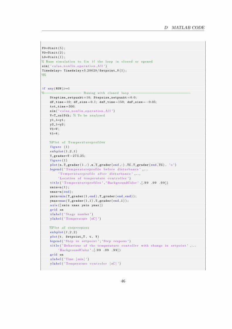
D Matlab code
%−−−−−−−−−−−−−−−−−−−−−−−−−−−−−−−−−−−−−−−−−−−−−−−−−−−−−−−−−−−−−−−−−−−−−−−−−−%−−−−−−−−−−−−−−−−−−−−−−−−−−−−−−−−−−−−−−−−−−−−−−−−−−−−−−−−−−−−−−−−−−−−−−−−−−% S t a r t e r o f the D i s t i l l a t i o n c o l u m n
%<<<< >>>>%
% This f i l e can run both with open loop , to tune the c o n t r o l l e r based on %
% which opera t i on po int i s chosen , but a l s o with c l o s e d loop to s imulate %
% how c o n t r o l l e r handles d i s tu rbance s in f e ed ra t e and f eed compos it ion . %
% To choose between open and c l o s e d loop open s imul ink f i l e %
% ” c o l a s n o n l i n o p e r a t i o n A l l ” and change the p o s i t i o n o f the %
% ”Manual Switch ” by d o b b e l k l i c k i n g on i t . Then run t h i s f i l e %
% ” S t a r t e r A l l ” .
%<<<< >>>>%
c l c
c l e a r a l l
c l f
N=41; %Number o f s t a g e s
i=1:N ; n ( i )=i ; % Matrix with s t a g e s in i n c r e a s i n g order
Tb1=261.45; %Bo i l i ng po int o f i so−butane
Tb2=272.65; %Bo i l i ng po int o f n−butane
deltaTb= Tb1−Tb2 ; %Bo i l i ng po int d i f f e r e n c e
%I n i t i a l de lay in b o i l e r
Timedelay=2;
%TC
TC=15; %Locat ion o f TC, numbering from the bottum of the column
T_under=TC−1; %Stages under TC
T_control=1;
T_over=N−TC ; %Stages over TC
%I n i t i a l va lue s
tot_time=5;
Steptime=0; Stepsize=0; %Rebo i l e r
Steptime_setpunkt=0; Stepsize_setpunkt=0; %Setpo int in TC