SPECIFIC ENERGY YIELD OF LOW-POWER AMORPHOUS SILICON AND CRYSTALLINE SILICON PHOTOVOLTAIC MODULES IN A SIMULATED OFF-GRID, BATTERY-BASED SYSTEM HUMBOLDT STATE UNIVERSITY By Stephen Kullmann A Thesis Presented to The Faculty of Humboldt State University In Partial Fulfillment Of the Requirements for the Degree Master of Science In Environmental Systems: Energy, Environment, and Society May 2009
Transcript
SPECIFIC ENERGY YIELD OF LOW-POWER AMORPHOUS SILICON AND
CRYSTALLINE SILICON PHOTOVOLTAIC MODULES IN A SIMULATED
OFF-GRID, BATTERY-BASED SYSTEM
HUMBOLDT STATE UNIVERSITY
By
Stephen Kullmann
A Thesis
Presented to
The Faculty of Humboldt State University
In Partial Fulfillment
Of the Requirements for the Degree
Master of Science
In Environmental Systems: Energy, Environment, and Society
May 2009
SPECIFIC ENERGY YIELD OF LOW-POWER AMORPHOUS SILICON AND
CRYSTALLINE SILICON PHOTOVOLTAIC MODULES IN A SIMULATED
OFF-GRID, BATTERY-BASED SYSTEM
HUMBOLDT STATE UNIVERSITY
By
Stephen Kullmann
Approved by the Master's Thesis Committee:
_______________________________________________________________________ Arne Jacobson, Major Professor Date
_______________________________________________________________________ Charles Chamberlin, Committee Member Date
_______________________________________________________________________ Chris Dugaw, Committee Member Date
_______________________________________________________________________ Chris Dugaw, Graduate Coordinator Date
_______________________________________________________________________ Chris A. Hopper, Interim Dean Date Research, Graduate Studies & International Programs
iii
ABSTRACT
SPECIFIC ENERGY YIELD OF LOW-POWER AMORPHOUS SILICON AND
CRYSTALLINE SILICON PHOTOVOLTAIC MODULES IN A SIMULATED
OFF-GRID, BATTERY-BASED SYSTEM
Stephen Kullmann
Some amorphous silicon (a-Si) photovoltaic (PV) manufacturers claim that their
power ratings at standard test conditions (STC) understate the performance of their
modules because of a-Si technology’s ability to achieve 10-15% higher energy yield per
rated peak power (WP) than crystalline silicon (c-Si) technology. I tested this claim in a
simulated off-grid, battery-based system through a 12-month study of the energy yield of
five a-Si and five c-Si PV modules with ratings between 14 to 20 WP. The test was
conducted in Arcata California, with a climate characterized by mild, rainy winters and
dryer, often foggy, summers. The specific energy yield (energy yield per tested WP) of
the different types of modules was correlated to temperature, insolation, and clearness
index (C.I.) data and compared between the groups and between individual modules.
The a-Si group outperformed the c-Si group in specific energy yield (Wh/WP)
over the 12-month period by 2.7%. While it was statistically difficult to isolate the effects
of temperature and C.I. on specific energy yield, the results indicated that the a-Si
group’s higher specific energy yield is due more to better performance in higher
iv
temperatures rather than in low C.I. conditions. Two reasons that may account for a lower
difference in specific energy yield than reported in previous studies are Arcata’s mild
climate and the absence of a maximum power point tracker in the system. Both the best
and worst performing individual modules were a-Si, which illustrates that individual
module quality can outweigh any improved performance of a-Si technology.
v
ACKNOWLEDGEMENTS
Many people were instrumental in helping me complete this project. First, I would
like to thank my advisor and friend Arne Jacobson for conceiving of the idea and
entrusting it to me, as well as for all of the guidance and instruction he gave me during
my less-than-the-shortest-distance-between-two-points pursuit of my Masters Degree.
Charles Chamberlin served on my committee and provided valuable insight
throughout the project. Sharon Brown was an original member of my committee and
helped conceptualize the project as a whole. After she moved away from the area, Chris
Dugaw stepped in to serve on my committee and helped bring this project to completion.
I have to thank everyone at the Schatz Energy Research Center who provided
technical and moral support during this project, particularly Scott Rommel who
masterminded the electronics of the array and shared in the frustrations of getting
everything running right. My fellow students were a continual source of inspiration and
amusement. Ranjit Deshmukh helped edit the data processing software, and Douglas
Saucedo’s brilliant data analysis and modeling skills were essential in the beginning
phases of the project. Without the aid of Marty Reed, Equipment Technician and all
around nice guy, the array would have fallen apart multiple times.
Thanks to my parents for providing support, encouragement, and patience through
my many years of schooling. Finally, thank you to my wife Allyson and our daughter
Leela for helping me stay focused on the important things in life.
vi
TABLE OF CONTENTS
ABSTRACT....................................................................................................................... iii
Comparison of Specific Energy Yields................................................................. 52
Correlations between Average Module Temperature, Clearness Index, and Specific Energy Yield ........................................................... 56
Temperature Coefficients...................................................................................... 62
1 The thirteen solar PV modules in the study array. Module 5a failed in November 2006 and was replaced by module 5b. Results from module 1 were not used in the analysis because it does not appear to have an anti-reflective coating....................................................................................................................19
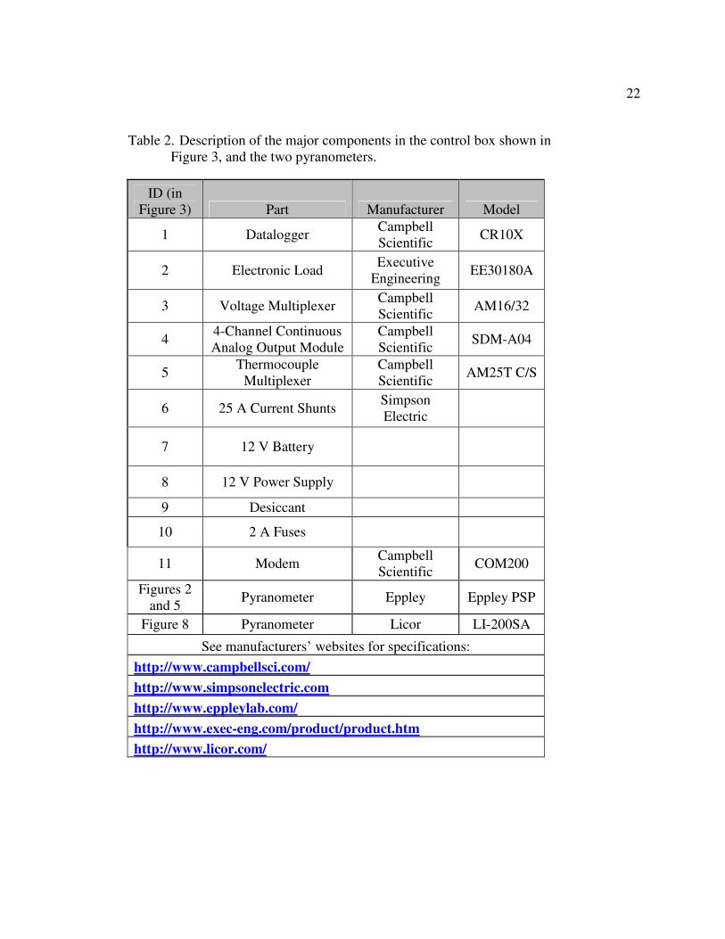
2 Description of the major components in the control box shown in Figure 3, and the two pyranometers. .....................................................................................22
3 Sensor equipment, ranges, and precisions. ............................................................27
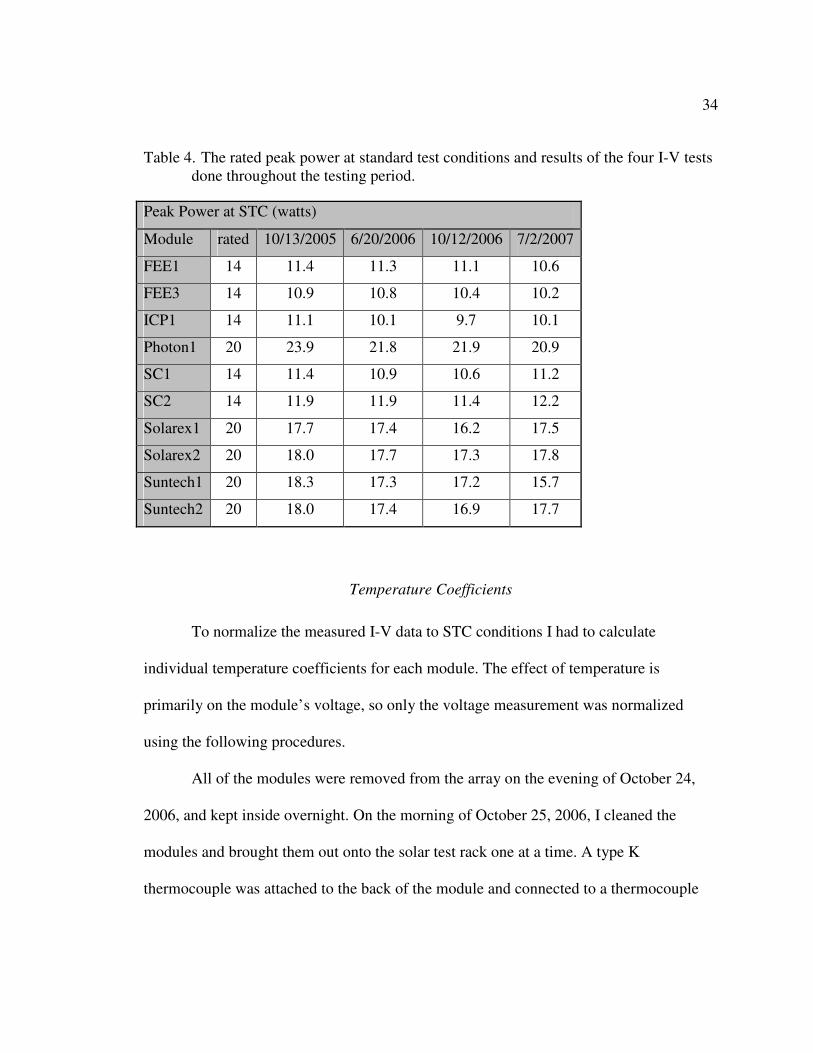
4 The rated peak power at standard test conditions and results of the four I-V tests done throughout the testing period. ...............................................................34
5 Temperature coefficients for the ten study modules. The c-Si group average is 19.2% lower than the a-Si group average. .............................................................36
6 Average, maximum, and minimum values of average ten-minute module temperature (Ta) and clearness index (C.I.) over the course of the 12-month testing period..........................................................................................................52
7 Summary of bins for 4x4 matrix, showing the upper and lower bounds, the count, and the percentage of total datapoints in each bin for average module temperature (Ta) (°C), and clearness index (C.I.), .................................................54
8 Coefficients and standard errors of 4x4 linear regression for percent difference in specific energy yield. The higher the coefficient, the more the a-Si group outperforms the c-Si group. Sample sizes are given in Table 7.............................56
9 Correlation test results suggesting little correlation between the factors of average modular temperature (Ta), clearness index (C.I.), or the product of the two variables and the difference in specific energy yield [(AveaSi – AvecSi)/AvecSi]between the two types of modules. ................................................57
10 Monthly and annual specific energy yield percent difference from mean for the individual modules and two groups. ................................................................64
ix
LIST OF FIGURES
Figure Page
1 Project location on the roof of the Science D Building, Humboldt State University in Arcata, California...............................................................................3
2 The project array, located on the roof of Science D building at Humboldt State University, showing the modules listed in Table 1......................................20
3 The control and datalogging box, with the main components numbered referring to their descriptions in Table 2................................................................23
4 View beneath the array showing the wiring of the thermocouples and modules positive and negative leads. The thermocouple sensors are attached to the center of the back of the modules and covered in insulating material.........24
5 Simple flowchart showing the data collection process for the PV array. For readability, the 12 PV modules and 4 shade sensors are grouped in the flowchart, but they are wired separately in the array. Major components are listed in Table 2. ....................................................................................................25
6 A cumulative probability diagram and histogram comparing the distributions of 31 days of simulated voltages and 300 days of randomly selected battery voltages as measured in 11 Kenyan off-grid PV systems............29
7 An I-V curve for module Solarex2, taken at the end of the year of data collection, July 2, 2007. Two runs are graphed with the data corrected for standard test conditions (25°C and 1000 W/m2). The peak power point (WP) is indicated by the dashed blue line. ......................................................................31
8 The author performing an I-V test on an a-Si PV module. ....................................32
9 Average monthly daytime a-Si, c-Si, and ambient temperatures. The a-Si group runs consistently hotter than the c-Si group. ...............................................46
10 Percent difference in average monthly specific energy yields between the a-Si and c-Si groups. The annual average percent difference is 2.7%......................48
x
11 Percent difference in monthly average specific energy yields [(Avea-Si – Avec-Si)/Aveall] versus average module temperatures. A positive value indicates the amount by which the a-Si outperformed the c-Si modules. The two outlier points below the trendline are from December 2006 and January 2007. ....................................................................................................................49
12 Percent difference in monthly average specific energy yields [(Avea-Si – Avec-Si)/Aveall] versus average daily insolation. A positive value indicates the amount by which the a-Si outperformed the c-Si modules..............................50
13 Distribution of average module temperature and clearness index (C.I.). The C.I. values over 1.0 occurred in two consecutive intervals in the late afternoon on May 2, 2007 and are most likely the result of an isolated incidence of cloud focusing of sunlight on the array. ............................................53
14 The percent difference in specific energy yield for each of the 16 bins with error bars reflecting one standard deviation. Positive values indicate percent by which the a-Si group outperforms the c-Si group. The percent difference is calculated as [(AveaSi – AvecSi)/AvecSi]..............................................................55
15 Four plots showing the four average module temperature (Ta) bins on a graph of clearness index (C.I.) versus percent difference in specific energy yield, with standard error bars shown. ...................................................................59
16 Four plots showing the four clearness index (C.I.) bins on a graph of average module temperature (Ta) versus percent difference in specific energy yield, with standard error bars shown. .............................................................................61
xi
LIST OF APPENDICES
Appendix Page
A COMMON ELECTRICAL TERMINOLOGY .....................................................71
B BATTERY VOLTAGE DATA ANALYSIS AND STOCHASTIC MODELING ..........................................................................................................74
C I-V CURVE SPREADSHEET...............................................................................88
D TEMPERATURE COEFFICIENTS TEST ...........................................................90
E SOLAR DATA PROCESSING CODE.................................................................93
F DAILY MONTHLY SUMMARIES ...................................................................103
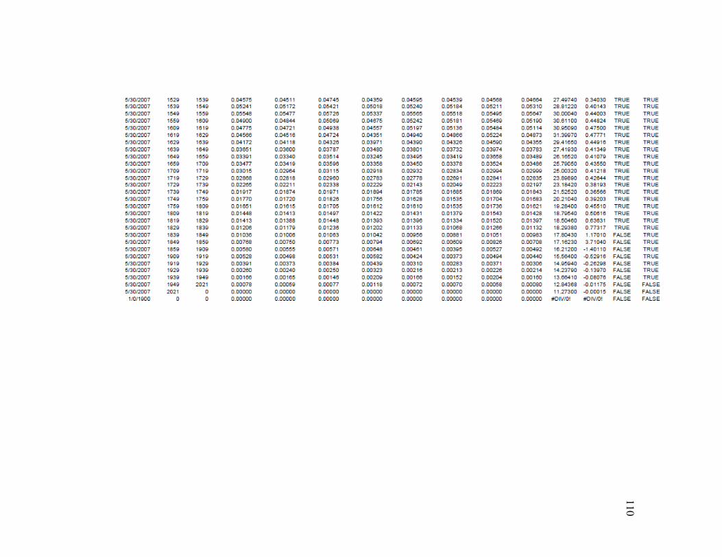
G CLEARNESS INDEX SPREADSHEET 2007.05.30 .........................................107
H 4X4 MATRIX REGRESSION SPREADSHEET ...............................................111
1
INTRODUCTION
As society recognizes the demand for clean, renewable energy, more effort is
placed on the improvement of technologies such as solar photovoltaic (PV) modules.
Two common types of modules are crystalline silicon (c-Si) and amorphous silicon
(a-Si). Ratings for PV modules are generally reported as peak power (WP) for standard
test conditions (STC) of 1000 watts per square meter (W/m2) insolation direct normal to
the module and 25ºC, measured in a controlled laboratory setting. Real-world conditions
rarely match the testing laboratory conditions exactly, so it can be difficult to accurately
predict how an individual or type of module will perform in particular light and
temperature conditions. Some a-Si PV manufacturers claim that their STC power ratings
understate the real-world performance of their modules because of a-Si technology’s
ability to achieve 10-15% higher specific energy yield, the energy yield per WP, than c-Si
technology, due to higher relative efficiencies both in diffuse light and at higher
temperatures (Jacobson and Kammen, 2007, Van Cleef, 2001, Jansen, 2006).
Having a rating system that accurately reflects the expected energy yield of a PV
module is important because consumers may wish to use the ratings to compare different
products. Inaccurate ratings, whether because of the differences in technologies or poor
quality control, may affect the acceptance of PV as a viable energy source. The typical
user will not know if the rating of the module is accurate, only if the system is producing
sufficient energy. In addition to any differences in the energy yield of the different
2
technologies, the measured peak power of most of the modules in this project was lower
than their nominal ratings.
I conducted a 12-month study of the energy yield of ten low-power PV modules
in a simulated off-grid, battery-based system. The study included five a-Si and five c-Si
modules with ratings between 14 to 20 WP. All of the amorphous modules were single
junction a-Si PV technology, while the c-Si modules included a mix of monocrystalline
and polycrystalline technologies. I measured the actual peak power for each of the
modules and calculated the specific energy yield, defined as energy yield per tested peak
power. The specific energy yield was correlated to temperature, insolation, and clearness
index (C.I.) data and comparisons were made between the two groups and among the
individual modules.
The project array location was on the roof of the Science D Building at Humboldt
State University in Arcata, California (see map in Figure 1). Arcata is located in coastal
Northern California and has a climate characterized by mild, rainy winters and dryer,
often foggy, summers.
Twelve months of data, from July 2006 through June 2007, were used for this
analysis. Data collection occurred every minute of daylight hours for the voltage, current,
and temperature of each module, as well as ambient temperature, total solar insolation
(power from the sun in W/m2), and the voltage setpoint for the array. The voltage setpoint
also changed every 30 minutes controlled by an algorithm based on battery voltages
directly measured in small off-grid Kenyan systems.
3
Figure 1. Project location on the roof of the Science D Building, Humboldt State University in Arcata, California.
4
Two methods were used to analyze the data and report the findings. First, sums of
daily average specific energy yield were reported for each month. These data show the
a-Si group outperforming the c-Si group in the months of April through October by a
small margin. The largest difference in specific energy yield between the two groups was
7.4% in July. The a-Si group is equal to or slightly below the c-Si group in November
through March. The a-Si group also outperformed the c-Si group on average over the
entire year by 2.7%. This suggests that while the a-Si modules in this study show a
definite advantage over the c-Si modules in specific energy yield, the cause is more likely
due to better performance in higher temperatures experienced in the summer months than
any benefit in diffuse light conditions.
To further examine the effects on specific energy yield from temperature and
diffusivity, the data were separated into nearly 20,000 ten-minute intervals through the
year. The clearness index was calculated for each of the intervals by taking the ratio of
the solar energy measured by the pyranometer at the array and the available solar energy
at the same tilt at the edge of the atmosphere. The intervals were divided into a four-by-
four matrix of average module temperatures (Ta) and clearness index. The a-Si group
outperformed the c-Si group across the range of temperatures and clearness indexes
except for in the bin with the lowest Ta and C.I. values.
As in the monthly analysis, the a-Si group had an average specific energy yield
2.7% higher than the c-Si group over the 12-month period. Temperature appeared to play
a greater role in the a-Si group’s improved performance than clearness index, although
5
the two effects are difficult to isolate statistically. The mild temperatures of the testing
location may have contributed to the small relative difference between the two groups.
Furthermore, the worst individual performer was an a-Si module, so the
differences between modules may be greater than the differences between groups. This
study presents no clear support for a different rating system for a-Si modules alone. An
overall change in the rating system for all PV modules that more accurately predicts the
expected energy yields could be warranted. Finally, failure of one out of the twelve
original modules and the low tested to rated peak power ratio for all of the modules both
call for greater diligence in the manufacture and testing of low power PV modules sold in
markets like they are in Kenya. In addition to what was learned from the data collection,
we have also acquired considerable knowledge and experience in conducting long-term
PV tests and will be able to build on that experience for future testing projects and make
it available to others wishing to conduct similar experiments.
This project is a continuation of the work performed by my advisor, Dr. Arne
Jacobson, in his Ph.D dissertation (Jacobson 2004), and in subsequent research (Jacobson
and Kammen, 2007). My involvement in the project began as a graduate student research
assistant at the Schatz Energy Research Center (SERC) at Humboldt State University in
2006. Dr. Jacobson had conceived of an idea to test a-Si solar module manufacturer’s
claims that their modules had higher specific energy yields in high temperature and
diffuse light conditions. I was involved in all aspects of the project, from the design,
6
construction, and wiring of the test array through the day-to-day maintenance, trouble-
shooting, and data collection, to the final analysis and reporting of the data.
The next chapter is a literature review with discussions on the research leading up
to this project, how PV works, and previous energy yield tests. The remainder of this
thesis report consists of a discussion of the methodology, the results of the data analysis,
and conclusions and recommendations. A glossary of some common electrical
terminology used throughout this thesis report is included as Appendix A. Appendices B
through H contain background material and sample spreadsheets used in the analyses.
7
LITERATURE REVIEW
This chapter begins with an introduction to how PV works and some of the
differences between a-Si and c-Si technologies. Next is a discussion of research on the
issues of PV product quality in Kenya, which provides much of the background for this
thesis project. Following is a review of some of the applicable research done on the
energy yields of specific PV technologies, both by independent research laboratories and
in manufacturer-sponsored reports.
How PV Works
Photovoltaic modules directly convert the sun’s power into electricity. This
section will provide a brief description of how photons from the sun are converted into
electricity that can be used to power loads or charge batteries.
A PV cell is made up of two or more layers of a semiconductor material, most
commonly silicon. The layers are intentionally doped with impurities, generally
phosphorous and boron. The silicon layer doped with phosphorous is called n-type and
has extra electrons. The boron layer is called p-type and has fewer electrons. When struck
by a photon of sunlight, an electron is freed and travels from one layer to the other. The
electron is directed through a path along positive and negative leads to flow through a
circuit to return to its original layer. This flow of electrons through a circuit produces a
current, which is electricity that can be used to power loads. In addition to the silicon
8
layers, a typical solar module will also have a protective glass cover, an anti-
reflective coating, and contact grid layers (US Department of Energy 2006).
A c-Si module is made up of a number of pairs of thin slices of crystals wired
together in parallel (positive connected to positive, negative connected to negative) to
increase the voltage. An a-Si module is composed of a non-crystalline form of silicon
layered in thin sheets. Amorphous silicon modules require less energy input to produce,
resulting in lower costs. Crystalline silicon modules have greater efficiencies than a-Si
modules in terms of power output per surface area. This means that to have the same
power output, an a-Si module would need to be larger than a c-Si module of the same
rating. In terms of cost per watt they would be approximately equal or the a-Si may be
somewhat less. (US Department of Energy, 2006).
Amorphous silicon modules experience an initial period of performance drop,
known as Staebler-Wronski degradation, during their first few months of exposure to
sunlight. The amount of degradation and time before stabilization varies between
manufacturers, so it is often difficult to predict an a-Si module’s stabilized performance
from its initial performance (Staebler and Wronski, 1977, cited in Duke, et al., 2002, and
Jacobson and Kammen, 2007). The a-Si modules in this project were all given a “light-
soaking” period until their measured peak power output stabilized.
Kenyan Solar
The background for my thesis project stems from Arne Jacobson’s research into
the Kenyan solar PV market. In Jacobson and Kammen (2007), the authors discuss issues
9
in the Kenyan PV market and the results of tests of PV modules commercially
available in Kenya.
Kenya has one of the largest per capita solar markets in the developing world, but
little oversight has led to concerns about product quality. Five brands of a-Si solar
modules available in the Kenyan market were tested in 2004 and 2005 to compare their
post light-soaking peak power to the manufacturers’ ratings. Two of the five modules
performed well below their rated specifications, while three were measured near 12 W for
a 14 W rating. The manufacturers had already said that the correct stabilized power
output for their modules was 12 W, so the performance corresponded to expectations.
Nonetheless, the modules were being sold on the Kenyan market with a 14 W rating.
Jacobson and Kammen’s article also reports on the authors’ tests of Kenyan solar
modules in 1999, which resulted in the removal of some underperforming brands from
the market, and encouraged other brands to improve their product.
Energy Yield Tests
Some of the a-Si manufacturers claim that brands of a-Si modules have been
shown to produce 15% more energy per rated WP than c-Si modules. In Van Cleef, et al.
(2001), the authors observed up to 20% higher energy yield per peak power and attribute
this to higher performance in diffuse light and high temperature, and greater tolerance for
shading. Tests are cited that indicate higher relative performance by not only the Uni-
Solar triple junction a-Si modules, but also show single-junction a-Si modules
outperforming c-Si modules.
10
These claims are based primarily on a Dutch study by Eikelboom and
Jansen (2000) using indoor and outdoor tests conducted on nine solar modules of
different technologies. I-V curves were taken at a number of temperatures and irradiances
using a test rig with a mobile robot positioner and were used to calculate module
efficiencies, defined as the ratio between output power and incident irradiation on the
entire module area. The a-Si modules were tested pre-degradation and were scaled to
yield manufacturer specified nominal power. An indoor flash tester was used to also
produce I-V curves as well as temperature coefficients. The resulting data were used in a
computer model to estimate annual energy yields per stated peak power.
The modules with the highest specific energy yields (kWh/kWP) were both a-Si
technology. The researchers attribute the high performance of the a-Si modules to their
low temperature coefficients and excellent low light level characteristics.
The results of the Dutch study (Eikelboom and Jansen, 2000) are questionable for
several reasons. The methodology for estimating the performance in low light conditions
involved tilting the modules away from the sun, which does not accurately simulate all
low light conditions. The energy yield data are determined through an untested model as
opposed to direct measurements. The a-Si modules were tested pre-Staebler-Wronski
degradation, and the peak power was scaled to manufacturers’ stated ratings in a way that
may not accurately reflect performance. The researchers also provide the disclaimer that
the modules used were not all purchased on the free-market, which allows for the
possibility of manufacturers “cherry-picking” their best modules for testing. They also
11
state that the number of modules in the study is too small to draw any general
conclusions. Finally, independent studies by other researchers have not replicated
Eikelboom and Jansen’s results.
The following study benefits from being a direct comparison of energy output
instead of using a model. Jardine (2002) studied two solar arrays, one in London, UK,
and the other in Mallorca, Spain. Both arrays were made up of 11 subarrays of different
technologies, including triple, double, and single-junction a-Si, single and multi-junction
c-Si, copper indium diselenide (CIS), and cadmium telluride (CdTe) cells. The two arrays
were 6.2 kWP each, and the subarrays ranged from 512 to 640 WP each. The authors did
not report the number of modules in each subarray. The array in London was tested for
one year and the array in Mallorca was tested for two years. Data were recorded over the
course of the test periods and used to calculate specific energy yields.
The multi-junction a-Si and CIS subarrays were found to have the highest specific
energy yields, while the single junction a-Si and CdTe subarray had the lowest. They also
reported that a-Si modules in general perform better than c-Si modules under high
temperatures and diffuse lighting, while c-Si modules perform better in low temperature
conditions.
Testing a wide variety of modules in different locations set up in subarrays helps
instill confidence in the comparison between technologies. While all a-Si modules were
found to benefit from high temperature and diffuse light effects, only the multi-junction
a-Si modules showed an overall higher energy yield than c-Si modules. The authors
12
stated that due to potential inaccuracies from manufacturers’ rated peak power,
insolation measurements, and inverter power levels, the absolute energy yield values they
report may be inaccurate. They attest that the conclusions about the physical responses of
the different technologies still hold true. Furthermore, the London array was installed at a
tilt of 13° and orientation of 5° W of south. The Mallorca array was at a 25° tilt and
orientation 15° W of south. Both of the arrays were tilted at a sub-optimal angle that
would benefit performance in the hotter summer months when the sun is higher in the
sky. This could lead to overall specific energy yield performance results favoring a-Si
modules.
The overall energy yield advantage for a-Si modules is contradicted by Fairman,
et al. (2003), who report on a year-long study conducted in a desert climate in Israel
testing the energy yield of a-Si and c-Si modules. Both mono and polycrystalline c-Si
modules were used. Monthly hourly energy yield averages, irradiance data, and measured
peak power output were used to calculate system efficiency and specific energy yield.
The results showed higher specific energy yields (termed specific energy delivery) for the
a-Si modules throughout the months from March through September, with the c-Si
modules performing slightly better for the rest of the year. The data were then examined
on an hourly basis for the months of March, June, September, and December. For the first
three months, the a-Si modules outperform the c-Si modules during the mid hours of the
day, while for all hours in December and the morning and evening hours for the entire
year, the c-Si modules performed better. Overall, both the multi and mono-c-Si modules
13
had a higher specific energy yield than the a-Si modules, though the difference
was only 3% from highest to lowest. The authors attribute the differences between the
modules types to spectral shifts in light and temperature effects. The two effects are
related and not isolated in this study. This report uses the measured peak power values
rather than the rated values, which makes it similar to my project. The data are examined
only on a monthly basis for the year and hourly for four months. Temperature and
insolation conditions are presumed by time of day and year rather than from actual
measurements. These shortcomings make it difficult to accurately assess the effects of
temperature and insolation on specific energy yield, although it should not affect annual
results. Considering the evidence for a temperature effect on a-Si modules specific
energy yields, especially through direct measurements of temperature coefficients, it is
surprising that the warmer desert climate did not produce higher results for the a-Si
modules.
While the studies cited above have conflicting results, the evidence builds that
peak power at STC alone does not accurately predict the energy yield of different
technology PV modules. A case is made for a photovoltaic rating system based on energy
yield over a range of temperatures and insolation rather than peak power at standard test
conditions in two recent articles by Kenny, et al. (2005 and 2006). Tests were made in the
laboratory and then specific climatic data were used to make energy predictions. Energy
yield data were then collected for the same modules over the course of the year and
compared to the energy yield predictions, with favorable results. The goal of the
14
experiment was to develop an energy yield rating system that would be both
relatively simple to execute while more accurately predicting performance than the
current STC rating system. For simplicity, the authors did not consider effects of light
diffusivity or spectral differences.
They concluded that using only insolation and temperature data is not sufficient to
accurately predict the energy yield of thin film PV modules, and that the effects of
spectral variations must be accounted for. The tests are conducted by taking multiple I-V
curve measurements throughout the day while the module is mounted on a solar tracking
device to keep it oriented directly normal to the sun. The purpose of the solar tracker is to
negate any effect of angle of incidence. The spectral variations are calculated from the
amount of air mass the sunlight must pass through at the time of the test. The results
show that the performance of the thin film modules is influenced by changes in the solar
spectrum. Accounting for changes in the solar spectrum in energy yield is difficult,
however, because haze and clouds significantly modify the spectrum and are difficult to
predict.
The multi-junction a-Si and CIS modules were the best performers in specific
energy yield. The a-Si modules overall performed better in higher temperatures, while the
c-Si modules performed better at lower temperatures. As in other studies, this study used
the manufacturers’ rated peak power instead of the actual tested peak power.
An article by Drews, et al. (2008), discusses the use of irradiation maps to predict
the energy yield of PV installations based on their rated peak power. Ten PV installations
15
in the German state of Saxony ranging from 0.75 to 92 kWP of installed power
were tested. The specific energy yield (kWh/kW) was predicted using the irradiation
maps and compared to the actual specific energy yields. The relative errors between the
modeled and measured specific energy yields ranged from -7.3 % to 8.4%, with the mean
of absolute errors being 4.65%. This result shows the potential for inaccuracies in energy
yield predictions using rated peak power at STC and irradiation data and the need for a
more refined approach to rating PV modules.
Another example of an a-Si PV manufacturer claiming better energy yield
performance is found in an article by K.W. Jansen, et al. (2006). The study, published by
researchers at Energy Photovoltaics, Inc, an American subsidiary of a German PV
manufacturer, claims 18% greater specific energy yields for a-Si PV modules compared
to c-Si over the course of a one-year test in central Florida, with the greatest gains during
high temperature times. While the results coming directly from a manufacturer should be
interpreted with caution, the article is interesting in that it also calculates the total
installed cost for electricity. The cost for electricity for the a-Si arrays was calculated at
$0.168 - $0.190 /kWh compared to $0.203/kWh for the c-Si. The results are also in doubt
because they were based on the rated peak power of two nine-module a-Si arrays,
potentially hand-selected by the manufacturer, and a single, un-specified c-Si module.
Differences between this Project and Previous Research
My thesis project adds some different elements and procedures to the research
discussed above. This project investigates the energy yield of low-power modules in a
16
simulated battery-based, off-grid system. Previous studies concentrated on
higher power modules in grid-connected AC arrays. This difference will yield results
more applicable to the type of modules and available in markets in sub-Saharan Africa
and other “developing world” markets.
The voltage setpoint in this study was determined by a probability algorithm
based on actual recorded voltages from Kenyan households with battery-based PV
systems instead of the maximum power point trackers used in other studies. Maximum
power point trackers keep the voltage at the point that will maximize the product of the
current and voltage, resulting in peak power output (see the following chapter for more
discussion on calculating peak power from I-V curve measurements).
This study differs from previous research not only in the how the data are
collected, but how they are analyzed. Instead of calculating specific energy yield using
the rated peak power, as in most of the previously cited reports, I use my I-V curve test
results to calculate the modules’ actual peak power. The resulting specific energy yield
more closely compares differences in PV technology because inaccuracies in modules
ratings are removed as a contributing variable. Also, statistical methods are used to
attempt to isolate the effects of temperature and clearness index on the differences in
specific energy yield.
Finally, the climate in Arcata is also different than that in other studies. The mild,
foggy summers are likely a contributing factor in the smaller difference in specific energy
yields compared to some reported by other research.
17
METHODOLOGY
This chapter includes discussions of the mechanics of setting up the test array,
descriptions of the modules used, I-V solar module testing procedures, and the algorithm
for setting the module voltage operating points during the test. The collection, processing,
and analysis of the data are discussed in the data collection and analysis section at the end
of this chapter.
Description of Modules in the Project
Thirteen PV modules were tested throughout this project, with the data from ten
being used in the final analysis. The study initially began with twelve PV modules: six
a-Si and six c-Si. One of the a-Si modules, ICP-2, failed in November 2006 and was
removed from the array and replaced with another a-Si module, Sunsei-1. Data for these
two modules were not included in this report or in any of the averages. A decision was
made to not include data from the c-Si module Sangyug-1 because it does not appear to
have the same type of anti-reflective coating found on the other modules; this factor
could be a separate variable influencing its performance. All of the modules were
purchased on the open market in Kenya and represent the type of low-power modules
available for sale from different manufacturers and distributors. Detailed discussion of
solar PV market conditions can be found in Arne Jacobson’s Ph.D. dissertation
(Jacobson, 2004), and other research (Duke, et al., 2002; Jacobson and Kammen, 2007).
18
The thirteen modules used throughout this project, their specifications, country of
origin, and manufacturers’ ratings are listed in Table 1. All of the a-Si modules had been
light soaked for at least six months prior to their inclusion in this study and consecutive
I-V tests indicated that their maximum power had stabilized following Staebler-Wronski
degradation. (See the Literature Review chapter for more information on a-Si technology
and Staebler-Wronski degradation.)
Test Array
The test array was built in the spring of 2006. The twelve modules were mounted
on a wooden rack facing due south at a 41° tilt: this tilt angle is approximately equal to
the 40.87° latitude of the test site (Arcata, CA). Figure 2 is a photo of the array showing
the location of each of the modules. The modules were spaced so that both the two
groups of modules and modules of the same manufacturer would be spread out on the
array. Also, a wind block was constructed behind the array to prevent uneven cooling
from the breeze.
Positive and negative leads from each of the modules were connected to the
control and datalogging box, which is shown in Figure 3, with a description of the major
components in Table 2. Figure 4 is a photo from underneath the array showing the
module positive and negative leads and thermocouple wiring. Figure 5 provides a
simplified schematic of the overall system. The modules’ positive leads first pass through
a 2 amp fuse to protect the datalogging equipment, then to a bus bar connected to an
Executive Engineering EE30180A electronic load, regulated by a Campbell Scientific
19
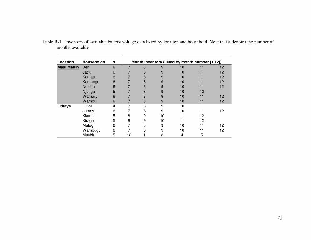
Table 1. The thirteen solar PV modules in the study array. Module 5a failed in November 2006 and was replaced by module 5b. Results from module 1 were not used in the analysis because it does not appear to have an anti-reflective coating.
Location Module ID Company/Brand Country Type WP Notes
1 Sangyug Sangyug Enterprises
India c-Si 15 Not included in analysis
2 Suntech 1 Suntech China c-Si 20
3 FEE 3 Free Energy Europe
France a-Si 14
4 Photon 1 Photon China c-Si 20
5a ICP-2 ICP Solar UK a-Si 14 Failed Nov. 2006. Not included in analysis
5b Sunsei 1 ICP Solar UK a-Si 14 Added Nov. 2006 to replace 5a. Not included in analysis
6 FEE 1 Free Energy Europe
France a-Si 14
7 SC-1 Solar Cells Croatia a-Si 14
8 Solarex 2 Solarex USA c-Si 20
9 Solarex 1 Solarex USA c-Si 20
10 SC-2 Solar Cells Croatia a-Si 14
11 ICP-1 ICP Solar UK a-Si 14
12 Suntech 2 Suntech China c-Si 20
20
Figure 2. The project array, located on the roof of Science D building at Humboldt State University, showing the modules listed in Table 1
Epply PSP Pyranometer Thermocouple with
radiation shield
Cooling fan for
electronic load
Control box
1
2
3
4
9 5
10 6
11 7
8 12
Module to
power cooling
fan
Additional
modules not
in this study
Shade
sensor 3
Shade
sensor 2
Shade
sensor 1
Shade
sensor 4
(out of
picture)
21
SDM A04 analog output module and controlled by a Campbell Scientific CR10X
datalogger. From there they are connected through 1:20 voltage dividers into a Campbell
Scientific AM16/32 voltage multiplexer, from where the voltage is recorded by the
datalogger.
The negative leads from the modules are wired into a series of Simpson Electric
25 amp current shunts across which the voltage drop is measured to calculate the current.
Type K thermocouples were secured with metallic tape to the back of each module and
covered in insulating material. The thermocouples were wired into the control box where
the temperature of each of the modules was recorded. The ambient temperature was
measured with a Type K thermocouple protected in a radiation shield. The four shade
sensors and Eppley PSP pyranometer are also wired into the datalogger. A Campbell
Scientific COM200 Modem was used to download the datapoints to a remote PC server.
Every minute the datalogger recorded the following general data: date, time,
ambient temperature, voltage setpoint, solar insolation, and control box temperature; and
the following module-specific data: voltage, current, and temperature. The datalogger had
a memory capacity for just over two day’s of data, and the data were downloaded to the
remote server once daily just after midnight. It was important to check the server
regularly to make sure the connection to the modem was functioning properly. The
downloaded and real-time data were scanned on a regular basis for any irregularities that
might indicate any equipment malfunctions. Other general maintenance included cleaning
the twelve modules and the Eppley PSP pyranometer on a weekly basis.
22
Table 2. Description of the major components in the control box shown in Figure 3, and the two pyranometers.
ID (in Figure 3) Part Manufacturer Model
1 Datalogger Campbell Scientific
CR10X
2 Electronic Load Executive
Engineering EE30180A
3 Voltage Multiplexer Campbell Scientific
AM16/32
4 4-Channel Continuous Analog Output Module
Campbell Scientific
SDM-A04
5 Thermocouple
Multiplexer Campbell Scientific
AM25T C/S
6 25 A Current Shunts Simpson Electric
7 12 V Battery
8 12 V Power Supply
9 Desiccant
10 2 A Fuses
11 Modem Campbell Scientific
COM200
Figures 2 and 5
Pyranometer Eppley Eppley PSP
Figure 8 Pyranometer Licor LI-200SA
See manufacturers’ websites for specifications:
http://www.campbellsci.com/
http://www.simpsonelectric.com
http://www.eppleylab.com/
http://www.exec-eng.com/product/product.htm
http://www.licor.com/
23
Figure 3. The control and datalogging box, with the main components numbered referring to their descriptions in Table 2.
5
2
1
3 4
6
7
8 9
10
11
24
Figure 4. View beneath the array showing the wiring of the thermocouples and modules positive and negative leads. The thermocouple sensors are attached to the center of the back of the modules and covered in insulating material.
Type K
Thermocouple
25
Figure 5. Simple flowchart showing the data collection process for the PV array. For readability, the 12 PV modules and 4 shade sensors are grouped in the flowchart, but they are wired separately in the array. Major components are listed in Table 2. .
26
Sensor Precision
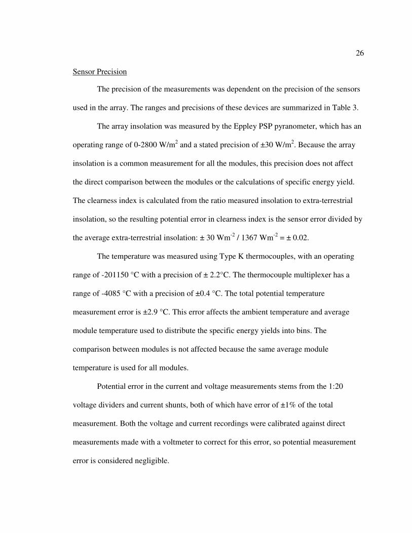
The precision of the measurements was dependent on the precision of the sensors
used in the array. The ranges and precisions of these devices are summarized in Table 3.
The array insolation was measured by the Eppley PSP pyranometer, which has an
operating range of 0-2800 W/m2 and a stated precision of ±30 W/m2. Because the array
insolation is a common measurement for all the modules, this precision does not affect
the direct comparison between the modules or the calculations of specific energy yield.
The clearness index is calculated from the ratio measured insolation to extra-terrestrial
insolation, so the resulting potential error in clearness index is the sensor error divided by
the average extra-terrestrial insolation: ± 30 Wm-2 / 1367 Wm-2 = ± 0.02.
The temperature was measured using Type K thermocouples, with an operating
range of -201150 °C with a precision of ± 2.2°C. The thermocouple multiplexer has a
range of -4085 °C with a precision of ±0.4 °C. The total potential temperature
measurement error is ±2.9 °C. This error affects the ambient temperature and average
module temperature used to distribute the specific energy yields into bins. The
comparison between modules is not affected because the same average module
temperature is used for all modules.
Potential error in the current and voltage measurements stems from the 1:20
voltage dividers and current shunts, both of which have error of ±1% of the total
measurement. Both the voltage and current recordings were calibrated against direct
measurements made with a voltmeter to correct for this error, so potential measurement
error is considered negligible.
27
Table 3. Sensor equipment, ranges, and precisions.
Equipment Range Precision
Eppley PSP Pyranometer 0-2800 W/m2 ± 30 W/m2
Type K Thermocouple -40 - 333 °C ± 2.2 °C
Thermocouple multiplexer -40 - 85 °C ± 0.4 °C
Simpson 25 A Current Shunts ± 1%
Voltage Dividers ± 1%
CR10X Datalogger ±2500 mV ±333µV
The Campbell Scientific CR10X datalogger has a precision of ±333µV in the full
scale input range of ±2500 mV. For a voltage measurement of 8 V, which records as 400
mV after the voltage dividers, the potential error is less than 0.1%.
Voltage Setpoints
Every 30 minutes, the voltage setpoint is changed based on a probability
algorithm developed from recordings of actual operating voltages. These operating
voltages were collected from multiple Kenyan battery-based off-grid PV systems by
Jacobson during 2003 (Jacobson, 2004). Battery voltages for fifteen household PV
systems in two communities were collected on five-minute intervals for periods ranging
from four to six months. Douglas Saucedo, a graduate student at HSU and research
assistant at SERC, created a random voltage setpoint generator based on the probability
28
distribution of the collected data. He used a stochastic model to generate voltage levels
that closely approximate the distribution of the sampled data, tested against 300 days of
randomly selected battery voltage data from 11 different households. See Appendix B for
a more detailed explanation of the battery voltage probability analysis. An Executive
Engineering E830180 electronic load controlled by a Campbell Scientific SDM A04
four-channel continuous analog output module regulated the voltage setpoint based on a
5th degree polynomial algorithm. A histogram and a cumulative probability graph of the
voltage setpoints for the simulation and measured battery voltages from in the Kenyan
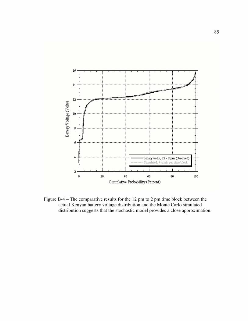
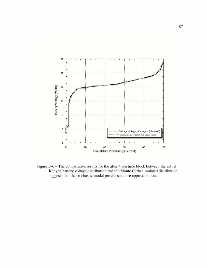
PV systems are shown in Figure 6. The distribution of the test system’s voltage setpoints
closely approximates the actual Kenyan battery voltage data.
I-V Curve Testing
To determine the actual peak power point (WP) of the individual PV modules, I-V
curve measurements were taken at regular intervals throughout the testing period. An I-V
curve is a plot of the modules’ current (I) in amperes (commonly shortened to amps) and
the voltage (V) in volts measured over a varying load or resistance. The test
measurements are normalized for the standard test condition (STC) temperature of 25º C
and insolation of 1000 W/m2. Current is affected primarily by changes in the insolation
29
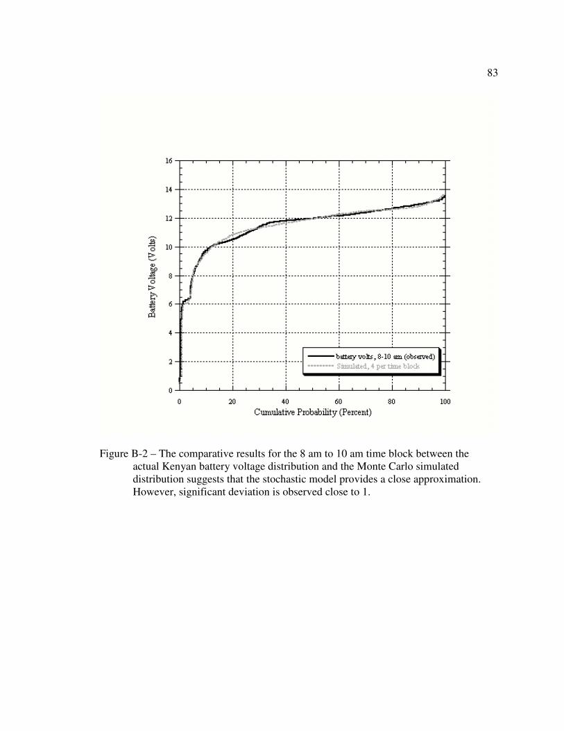
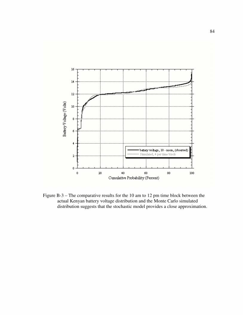
Figure 6. A cumulative probability diagram and histogram comparing the distributions of 31 days of simulated voltages and 300 days of randomly selected battery voltages as measured in 11 Kenyan off-grid PV systems.
striking the module, and voltage is affected primarily by the temperature, so current and
voltage are normalized for STC accordingly using Equations 1 and 2, respectively
(Chamberlin et al., 1995). The module temperatures during the I-V tests ranged from 48.1
to 65.4 °C, and the insolation ranged from 976 to 1037 W/m2.
=
E
mwII mn
2/1000
Equation 1
where: In = normalized current (A) Im = measured current (A) E = mean measured insolation on plane of PV module (W/m2)
{ })25( TCbVVV mmn −××+= o Equation 2
where: Vn = normalized voltage (V) Vm = measured voltage (V) b = temperature coefficient (1/°C) T = mean measured module temperature during test (°C)
The temperature coefficient is a measurement of the temperature effect on each
module and is described further in the next section. Current in amps multiplied by voltage
in volts equals power in watts (see Appendix A for a glossary of common electrical
terminology used in this report). Figure 7 shows an I-V curve for the module Solarex 2.
The peak power point is indicated with dashed lines, showing the rectangle with the
greatest area that can be inscribed beneath the curve. As shown in the sample I-V curve
in Figure 7, current is plotted against voltage producing a characteristic curve. The peak
31
power point is found near the knee of the curve, where amps multiplied by volts yields
the highest value for watts.
Figure 8 shows a typical I-V set up for one of the test modules. A sunny day, free
from haze and clouds, is chosen for the I-V test. The tests for the 12 modules are all
completed on the same day, in a time window near solar noon when the atmospheric air
mass, a measurement of the path length in the atmosphere sunlight needs to travel
through to reach the Earth’s surface, is less than two. The module is prepared for testing
0
0.2
0.4
0.6
0.8
1
1.2
1.4
0 5 10 15 20 25
Voltage (Volts)
Cu
rre
nt
(am
ps
)
Figure 7. An I-V curve for module Solarex2, taken at the end of the year of data collection, July 2, 2007. Two runs are graphed with the data corrected for standard test conditions (25°C and 1000 W/m2). The peak power point (WP) is indicated by the dashed blue line.
32
by removing it from the test array, cleaning it, and placing it on a test rack. The test rack
holds the module in the same plane as a Licor pyranometer, which has been calibrated
against the Eppley PSP pyranometer from the array, and uses a simple tube device to
allow the tester to orient the module’s surface directly normal to the sun. A type K
thermocouple is attached to each module to record the temperature. The positive and
negative leads of the module are connected to the variable resistive load and I-V tester.
The pyranometer and thermocouple are both connected to mulitmeters. The rack is then
Figure 8. The author performing an I-V test on an a-Si PV module.
Laptop
PV Module
Fluke Multimeter for
Pyranometer Signal
Thermocouple
Reader (hidden)
module)
Licor Pyranometer
Pyramoneter
I-V Test Rack
I-V Datalogger
Variable
Load
Rheostat
33
oriented to be directly normal to the sun and the load is increased from ISC to VOC while
the average insolation and temperature are recorded by two mulitmeters. To ensure
precision, two runs are taken for each module. To smooth the curve and correct for the
possibility of missing datapoints, an 8th degree polynomial was fit to the curve. The
polynomial equation is used to compute values for voltage and current, and the peak
power point is determined from the maximum value of the product. A sample
I-V curve spreadsheet is included in Appendix C. See Jacobson, et al (2000) for a more
detailed description of the I-V testing method and equipment.
The ten modules were tested four times to measure their peak power output. The
first test occurred well before the data collection period, and other tests were conducted at
the beginning, middle, and end of the data collection period. The second set of I-V tests,
conducted just before the beginning of the test period on June 20, 2006, was used to
calculate the specific energy yield values. For an explanation as to why these maximum
power values were used, see the section titled Rated vs. Tested Maximum Power on page
43, later in this chapter.
Every module, except for the Photon, tested lower than the manufacturers’ STC
ratings. Table 4 shows the results of the four tests and rated peak power output for the ten
modules in the study. Lower test results than the rated peak power values indicate that the
module’s performance will be lower than claimed by the manufacturer. In the last test on
July 2, 2007, the tested peak power for six out of the ten modules rose by some amount.
34
Table 4. The rated peak power at standard test conditions and results of the four I-V tests done throughout the testing period.
To normalize the measured I-V data to STC conditions I had to calculate
individual temperature coefficients for each module. The effect of temperature is
primarily on the module’s voltage, so only the voltage measurement was normalized
using the following procedures.
All of the modules were removed from the array on the evening of October 24,
2006, and kept inside overnight. On the morning of October 25, 2006, I cleaned the
modules and brought them out onto the solar test rack one at a time. A type K
thermocouple was attached to the back of the module and connected to a thermocouple
35
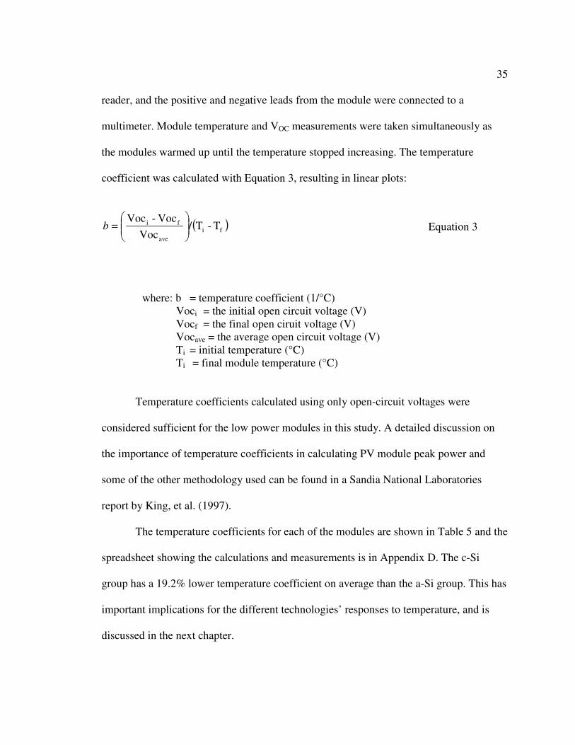
reader, and the positive and negative leads from the module were connected to a
multimeter. Module temperature and VOC measurements were taken simultaneously as
the modules warmed up until the temperature stopped increasing. The temperature
coefficient was calculated with Equation 3, resulting in linear plots:
( )fi
ave
fi T-T/Voc
Voc-Voc
=b Equation 3
where: b = temperature coefficient (1/°C) Voci = the initial open circuit voltage (V) Vocf = the final open ciruit voltage (V) Vocave = the average open circuit voltage (V) Ti = initial temperature (°C) Ti = final module temperature (°C)
Temperature coefficients calculated using only open-circuit voltages were
considered sufficient for the low power modules in this study. A detailed discussion on
the importance of temperature coefficients in calculating PV module peak power and
some of the other methodology used can be found in a Sandia National Laboratories
report by King, et al. (1997).
The temperature coefficients for each of the modules are shown in Table 5 and the
spreadsheet showing the calculations and measurements is in Appendix D. The c-Si
group has a 19.2% lower temperature coefficient on average than the a-Si group. This has
important implications for the different technologies’ responses to temperature, and is
discussed in the next chapter.
36
Table 5. Temperature coefficients for the ten study modules. The c-Si group average is 19.2% lower than the a-Si group average.
where: C.I. = Clearness Index IT = Extra-terrestrial solar radiation at tilt (Wh/m2) Io = Extra terrestrial flat plane solar radiation (Wh/m2) Ia = Solar radiation at array (Wh/m2) Rb = Tilt Factor θz = Zenith angle (degrees) θ = Angle of incidence (degrees) ω = Hour angle (degrees) calculated every minute. The subscripts 1 and 2 indicate the hour angles at the beginning and end of each interval. δ = Declination (degrees) E = Equation of time B = Day of year equation tsolar = Solar time tstd = Standard time n = Day of year = 1 to 365 β = Array tilt (degrees) = 41° Ф = Latitude at array (degrees) = 40.87° Lloc = Longitude at array (degrees) = 124.09° Lst = Standard meridian (degrees) = 120° Gsc = Solar Constant (W/m2) = 1367 W/m2 The ten minute intervals were checked for continuity (no missing data points
within the interval) and to ensure that the clearness index, angle of incidence, and zenith
angle all fall within appropriate ranges. The intervals were then imported into a new
spreadsheet where the resulting 19,916 datapoints were separated into a 4x4 matrix of 16
bins by temperature and clearness index (see spreadsheet excerpt in Appendix H).
Excel’s data analysis tools were used to analyze the data and the results are presented in
the Results and Discussion Chapter.
Rated vs. Tested Maximum Power
IV curves were measured for each of the tested modules to determine their actual
peak power output (WP) before, during and after the testing period. There was some
44
question as to which value for peak power to use for analysis. All of the modules tested
lower than their rated power, and most degraded to some degree during the testing period.
The specific energy yield (the ratio of energy yield over energy generating
potential) for the modules could be reported in multiple ways:
1. Wh/rated WP (WP r) 2. Wh/tested WP at the beginning of the test period (WP i) 3. Wh/tested WP at the end of the test period (WP f) 4. Wh/most recently tested WP through the test period (WP c)
This analysis is meant to test the energy yield between the two technologies, not the
accuracies of the manufacturers’ ratings, so using the manufacturers’ claimed peak power
value would not give an accurate representation of the modules’ actual energy yield
compared to its potential. Using the final or an average peak power value could
potentially reward the modules for degrading over the testing period, because a lower
peak power value would result in a higher specific energy yield value. The initial peak
power value was selected because it most accurately answers the question of how much
energy a module will yield compared to its potential. The degradation over time and the
inaccuracies in ratings are also interesting and are reported and discussed, but not used in
the analysis.
Note that all a-Si modules have an initial degrading period, and so all of the
modules were allowed to “light-soak” for a period of at least six months until their
measured peak power performance stabilized. See the Literature Review chapter for more
information on a-Si technology and Staebler-Wronski degradation.
45
Ambient vs. Module Temperatures
The temperatures of the individual modules as well as the ambient temperatures
were recorded. Careful attention was taken to construct and arrange the array so that the
two types of modules were spread out and not exposed to systematically and significantly
different weather and heat conditions. Higher temperatures reduce module efficiency and
energy yield, but manufacturers and some studies have suggested that this effect is lower
with a-Si than c-Si technology (see the Literature Review Chapter for more of this
discussion). Three different temperature values were considered for use in the analysis
for isolating the temperature effect on energy yield: i) ambient temperature, ii) average of
all module temperatures, and iii) individual module temperatures.
For an accurate comparison, the modules need to be compared at identical
conditions. The a-Si modules were consistently hotter than the c-Si modules in the same
ambient temperatures (see Figure 9). Therefore, if individual module temperatures were
used to examine the effect of temperature on specific energy yield, any reduction in
efficiency losses inherent to a-Si technology could be cancelled out by their higher
operating temperatures.
The efficiency of the modules is affected not directly by the ambient temperature,
but indirectly by the effect of the ambient temperature on the module temperature. It is
the physical properties of the materials and their temperatures that cause losses in
efficiency, not the temperature of the air surrounding them. The module temperatures can
not respond immediately to fluctuations in ambient temperatures; the thermal mass in
their materials would take some amount of time to release or absorb heat. Therefore, the
46
average of all module temperatures was selected to examine how the specific energy
yield is affected by the operating temperature. The ambient temperature may have brief
fluctuations while the modules may take longer to heat up or cool down. Using the
ambient temperature could potentially misrepresent the actual operating temperatures of
the modules when such instances occur. Examples of such potential instances are when a
cloud briefly obstructs the sun but the modules remain warm or in the morning when the
sun heats the air faster than the air heats the modules.
0
5
10
15
20
25
30
35
40
45
Jul-06
Aug
-06
Sep-0
6
Oct
-06
Nov
-06
Dec
-06
Jan-
07
Feb
-07
Mar
-07
Apr
-07
May
-07
Jun-0
7
annua
l avg
Tem
per
atu
re (
°C)
.
c-Si
a-Si
ambient
Figure 9. Average monthly daytime a-Si, c-Si, and ambient temperatures. The a-Si group runs consistently hotter than the c-Si group.
.
47
RESULTS AND DISCUSSION
In this chapter I present the results of the average and annual specific energy
yields of the two groups of modules, their performance as a function of operating
temperature and clearness index, and the specific energy yield performance of the
individual modules. Please refer to the Methodology Chapter for a detailed description on
these data analyses.
The a-Si group is shown to have a 2.7% higher annual specific energy yield on
average than the c-Si group. The a-Si group performed better in the warmer summer
months relative to the c-Si group, and equal to or poorer than the c-Si group for the rest
of the year. This suggests that higher temperature has a stronger correlation than low
clearness index to the improved specific energy yield of a-Si over c-Si PV technology.
The examination of the smaller interval datasets confirms, though not conclusively, this
result. The analysis of the specific energy yield of the individual modules shows the
deviance between individual panels to be greater than that between groups. Individual
module quality can negate any advantages a-Si technology has over c-Si technology in
relative energy yield performance.
Monthly Average Specific Energy Yield
Using monthly outputs from the SDC program, I calculated average daily specific
energy yield for each month (excerpts from the Daily Monthly Summaries spreadsheet
are included in Appendix F). Figure 10 is a graph of the percent difference in average
48
monthly specific energy yields between the a-Si and c-Si groups. The a-Si modules
outperform the c-Si on average over the entire year by a 2.7% margin. The summer
months have the highest difference in specific energy yield between the two groups, with
July the highest at 7.4%. The c-Si group outperforms the a-Si group in December,
January, and February. This suggests that while the a-Si modules in this study show an
advantage over the c-Si in specific energy yield, the cause is more likely due to better
performance in higher temperatures experienced in the summer months than any benefit
in diffuse light conditions.
-5%
-4%
-3%
-2%
-1%
0%
1%
2%
3%
4%
5%
6%
7%
8%
Ju
l-06
Aug-0
6
Sep
-06
Oct-
06
Nov-0
6
Dec
-06
Jan
-07
Feb
-07
Mar-
07
Apr-0
7
May-0
7
Ju
n-0
7
% D
iffe
ren
ce in
Sp
ecfi
c E
ner
gy Y
ield
.
annual average (2.7%)
Figure 10. Percent difference in average monthly specific energy yields between the a-Si and c-Si groups. The annual average percent difference is 2.7%.
49
To further isolate the effects of temperature and clearness on the specific energy
yield of the two groups of modules, I plotted the percent difference of average specific
energy yields between the a-Si and c-Si groups versus the average module temperatures
(Figure 11) and versus average daily insolation measured on the plane of the array
(Figure 12). The similar appearance of both plots is a result of the strong correlation
between temperature and insolation. As both the temperature and insolation increase, so
R2 = 0.50
-6%
-4%
-2%
0%
2%
4%
6%
8%
10%
20 22 24 26 28 30 32 34 36 38 40
Average Module Temperature (°C)
% D
iffe
ren
ce in
Sp
ecif
ic E
ner
gy Y
ield
Figure 11. Percent difference in monthly average specific energy yields [(Avea-Si – Avec-Si)/Aveall] versus average module temperatures. A positive value indicates the amount by which the a-Si outperformed the c-Si modules. The two outlier points below the trendline are from December 2006 and January 2007.
50
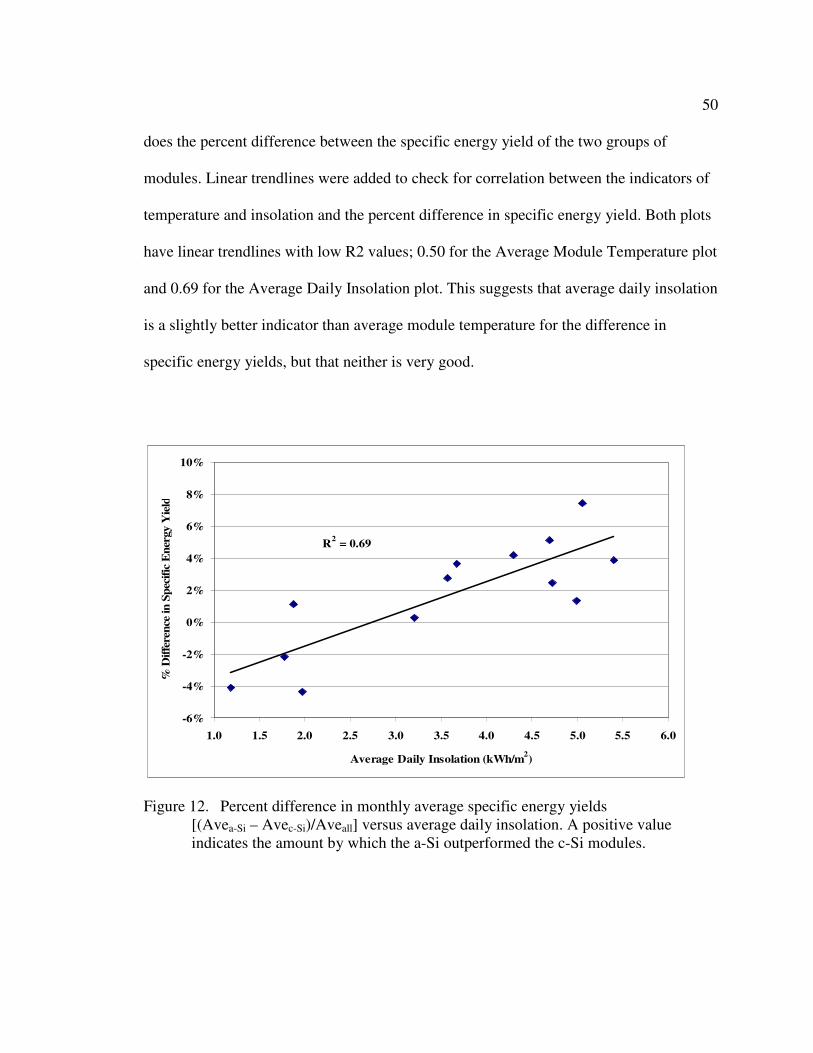
does the percent difference between the specific energy yield of the two groups of
modules. Linear trendlines were added to check for correlation between the indicators of
temperature and insolation and the percent difference in specific energy yield. Both plots
have linear trendlines with low R2 values; 0.50 for the Average Module Temperature plot
and 0.69 for the Average Daily Insolation plot. This suggests that average daily insolation
is a slightly better indicator than average module temperature for the difference in
specific energy yields, but that neither is very good.
R2 = 0.69
-6%
-4%
-2%
0%
2%
4%
6%
8%
10%
1.0 1.5 2.0 2.5 3.0 3.5 4.0 4.5 5.0 5.5 6.0
Average Daily Insolation (kWh/m2)
% D
iffe
ren
ce in
Sp
ecif
ic E
ner
gy Y
ield
Figure 12. Percent difference in monthly average specific energy yields [(Avea-Si – Avec-Si)/Aveall] versus average daily insolation. A positive value indicates the amount by which the a-Si outperformed the c-Si modules.
51
Ten-Minute Intervals
Using output from the SDC program, I calculated specific energy yields for each
of the modules for every minute of data collection. Using the methodology described in
the previous chapter, I also calculated a clearness index and average module temperatures
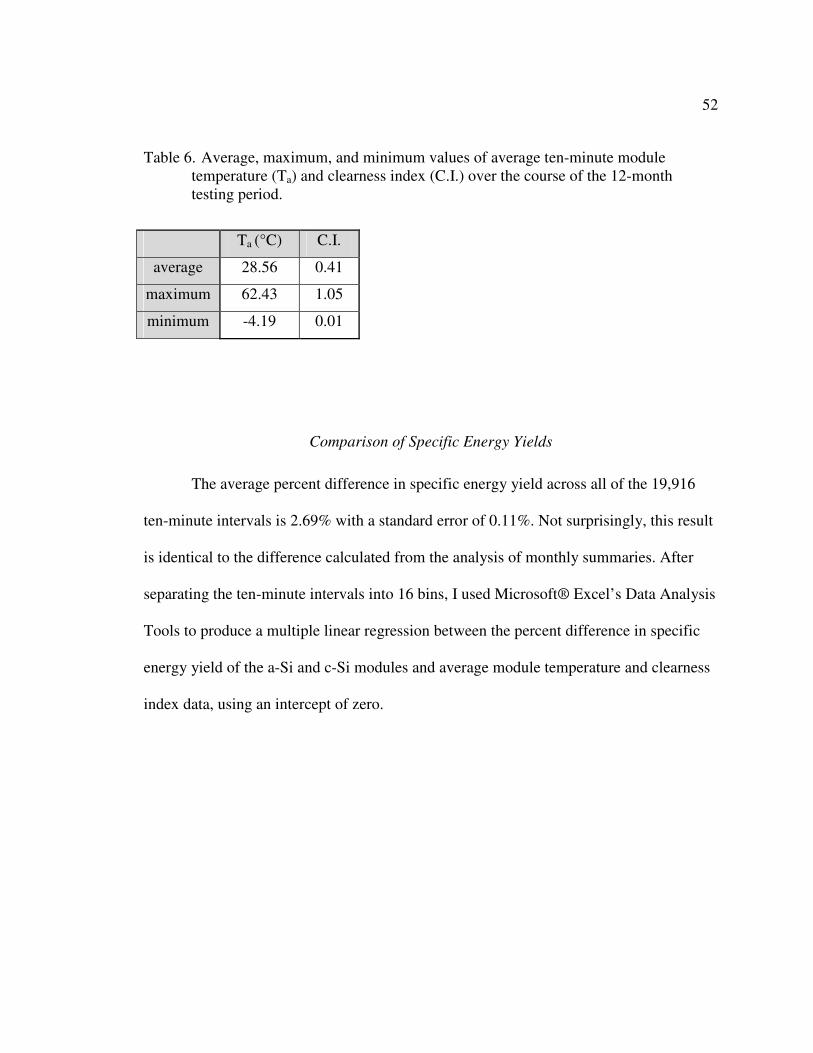
for each minute. The temperature and clearness index ranges are shown in Table 6. The
average module temperature ranges from -4.19 to 62.43 °C with a mean of 28.56 °C. The
range of clearness indexes is from 0.01 to 1.05 with a mean value of 0.41. The clearness
index values over 1.0 occurred in two consecutive ten-minute intervals in the late
afternoon on May 2, 2007 and are most likely the result of an isolated incident of cloud
focusing of sunlight on the array.
I divided the data into 19,916 ten-minute intervals and created a 4x4 matrix of
average module temperature and clearness index. Figure 13 shows a plot of clearness
index versus average module temperature with the 16 bins indicated. Table 7 lists the
upper and lower bounds of average module temperature and clearness index for each of
the 16 bins, the count of datapoints in each bin, and the percentage of the total for each
bin. Bin 2,1 is the highest frequency bin, with 21.02 % of the total intervals, and three
bins have less than 0.1 %, including bin 4,1 with no values.
52
Table 6. Average, maximum, and minimum values of average ten-minute module temperature (Ta) and clearness index (C.I.) over the course of the 12-month testing period.
Comparison of Specific Energy Yields
The average percent difference in specific energy yield across all of the 19,916
ten-minute intervals is 2.69% with a standard error of 0.11%. Not surprisingly, this result
is identical to the difference calculated from the analysis of monthly summaries. After
separating the ten-minute intervals into 16 bins, I used Microsoft® Excel’s Data Analysis
Tools to produce a multiple linear regression between the percent difference in specific
energy yield of the a-Si and c-Si modules and average module temperature and clearness
index data, using an intercept of zero.
Ta (°C) C.I.
average 28.56 0.41
maximum 62.43 1.05
minimum -4.19 0.01
53
Figure 13. Distribution of average module temperature and clearness index (C.I.). The C.I. values over 1.0 occurred in two consecutive intervals in the late afternoon on May 2, 2007 and are most likely the result of an isolated incidence of cloud focusing of sunlight on the array.
54
Table 7. Summary of bins for 4x4 matrix, showing the upper and lower bounds, the count, and the percentage of total datapoints in each bin for average module temperature (Ta) (°C), and clearness index (C.I.),
Figure 14 is a graph of the results of the linear regression showing the estimated
percent difference in specific energy yield between the a-Si and c-Si groups for each of
the 16 bins, with the associated one standard deviation error bars. For each of the ten-
minute intervals, the percent difference in specific energy yield is calculated as (AveaSi –
AvecSi)/AvecSi. Positive values indicate the percentage amount the a-Si modules
outperform the c-Si modules on average in specific energy yield. The same data are
presented in a tabular format in Table 8.
55
The a-Si group outperforms the c-Si group in all but one of the bins. The biggest
difference is seen in Bin 2,3, at over 10%. Bin 2,3 represents the middle-low Ta range
(15-30 °C) and the middle-high C.I. range (0.5-0.75). The only bin in which the specific
energy yield of the c-Si group is more than the a-Si group is Bin 1,1; the lowest Ta and
C.I. bin. The specific energy yield for Bins 1,4 and 2,4 are not statistically significantly
different from zero in terms of standard error, and Bin 4,1 has no datapoints.
-6%
-4%
-2%
0%
2%
4%
6%
8%
10%
12%
14%
bin
1,1
bin
1,2
bin
1,3
bin
1,4
bin
2,1
bin
2,2
bin
2,3
bin
2,4
bin
3,1
bin
3,2
bin
3,3
bin
3,4
bin
4,1
bin
4,2
bin
4,3
bin
4,4%
Dif
fere
nce
in
Sp
ecif
ic E
ner
gy
Yie
ld
Figure 14. The percent difference in specific energy yield for each of the 16 bins with error bars reflecting one standard deviation. Positive values indicate percent by which the a-Si group outperforms the c-Si group. The percent difference is calculated as [(AveaSi – AvecSi)/AvecSi]
56
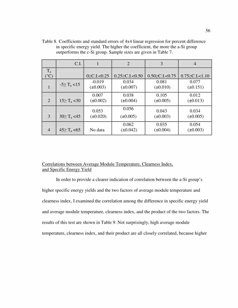
Table 8. Coefficients and standard errors of 4x4 linear regression for percent difference in specific energy yield. The higher the coefficient, the more the a-Si group outperforms the c-Si group. Sample sizes are given in Table 7.
Correlations between Average Module Temperature, Clearness Index, and Specific Energy Yield
In order to provide a clearer indication of correlation between the a-Si group’s
higher specific energy yields and the two factors of average module temperature and
clearness index, I examined the correlation among the difference in specific energy yield
and average module temperature, clearness index, and the product of the two factors. The
results of this test are shown in Table 9. Not surprisingly, high average module
temperature, clearness index, and their product are all closely correlated, because higher
57
Table 9. Correlation test results suggesting little correlation between the factors of average modular temperature (Ta), clearness index (C.I.), or the product of the two variables and the difference in specific energy yield [(AveaSi – AvecSi)/AvecSi]
between the two types of modules.
% difference [(AveaSi – AvecSi)/AvecSi]
Ta C.I. Ta x C.I.
% difference: [(AveaSi– AvecSi)/AvecSi]
1.00
Ta 0.10 1.00
C.I. 0.15 0.86 1.00
Ta*C.I. 0.12 0.95 0.94 1.00
temperatures occur at times of higher clearness. The correlation results between the
percent difference in specific energy yield and any of the three factors are all under 0.2,
with the clearness index factor the highest at 0.15, the average module temperature factor
0.10, and the product of the two 0.12. Unfortunately, these results provide little help in
solving the riddle of what contributes to the higher specific energy yield of the a-Si
group.
58
Figure 15 is a series of four graphs plotting the four average module temperature
bins on a graph of clearness index versus percent difference in specific energy yield
between the two groups of modules. Error bars indicate the standard error from the linear
regression. The higher the percentage difference, the more the a-Si group outperforms the
c-Si group in specific energy yield.
The below 15°C plot begins with a -2% difference, indicating that the c-Si group
outperformed the a-Si group at the lowest average module temperature and clearness
index bin, and it shows an increase in the difference in specific energy yield as the
clearness index increases. The final data point on this curve has a high standard error
because of small sample size, so the leveling off of the tail at the end is not statistically
significant. The 15-30°C plot shows an increase in the difference as the clearness index
increases, until the highest clearness index when it drops. The 30-45°C and above 45°C
plots both show much more level curves around 5% difference in specific energy yields.
The effect of clearness index on the difference in specific energy yield is more
pronounced in the lower temperature conditions. The effect is that as clearness index
increases, so does the amount by which the a-Si group outperforms the c-Si group in
specific energy yield, at least until the highest clearness index bin. If the a-Si modules
had a benefit in more diffuse light conditions, indicated by a lower clearness index value,
the curve should have been reversed.
59
Figure 15. Four plots showing the four average module temperature (Ta) bins on a graph of clearness index (C.I.) versus percent difference in specific energy yield, with standard error bars shown.
< 15 °C
-5%
0%
5%
10%
15%
<0.25 0.25-0.50 0.5-0.75 >0.75
Clearness Index (C.I.)
% D
iffe
ren
ce i
n S
pec
ific
En
erg
y
Yie
ld
15-30 °C
-5%
0%
5%
10%
15%
<0.25 0.25-0.50 0.5-0.75 >0.75
Clearness Index (C.I.)
% D
iffe
ren
ce i
n S
pec
ific
En
erg
y
Yie
ld
30-45 °C
-5%
0%
5%
10%
15%
<0.25 0.25-0.50 0.5-0.75 >0.75
Clearness Index (C.I.)
% D
iffe
ren
ce i
n S
pec
ific
En
erg
y
Yie
ld
>45 °C
-5%
0%
5%
10%
15%
<0.25 0.25-0.50 0.5-0.75 >0.75
Clearness Index (C.I.)
% D
iffe
ren
ce i
n S
pec
ific
En
erg
y
Yie
ld
60
Figure 16 is a series of four graphs plotting the four clearness index bins on a
graph of average module temperature versus percent difference in specific energy yield
between the two groups of modules. Error bars indicate the standard error from the linear
regression. As in the plots in Figure 15, the higher the percentage difference, the more the
a-Si group outperforms the c-Si group in specific energy yield.
Except for the clearness index range of 0.50 – 0.75, the difference in specific
energy yield increases as average module temperature increases. The steepest curve,
indicating the most dramatic effect of average module temperature on specific energy
yield, comes in the lowest clearness index range. The percent difference in specific
energy yield between the two module groups in the lowest clearness index range goes
from the c-Si group outperforming the a-Si group by about 2% in the lowest average
module temperature bin, to the a-Si group outperforming the c-Si group by over 5% in
the third average module temperature bin. There are no datapoints in the highest average
module temperature, lowest clearness index bin. The clearness index range of 0.25-0.50
shows a lower increase in difference in specific energy yield, going from under 4% to just
over 5% from the lowest to highest temperatures. The highest clearness index range also
shows a steady increase. The lowest average module temperature point can be ignored
because the bin contains only a single datapoint and therefore has a high degree of error.
The C.I. range from 0.50 to 0.75 begins with an increase in the difference in specific
energy yield from the lowest to the second lowest average module temperature bins to
61
Figure 16. Four plots showing the four clearness index (C.I.) bins on a graph of average module temperature (Ta) versus percent difference in specific energy yield, with standard error bars shown.
<0.25
-5%
0%
5%
10%
15%
< 15 °C 15-30 °C 30-45 °C >45 °C
Average Module Tempe rature (Ta)
% D
iffe
ren
ce i
n S
pecif
ic E
nerg
y
Yie
ld
0.25-0.50
-5%
0%
5%
10%
15%
< 15 °C 15-30 °C 30-45 °C >45 °C
Ave rage Module Te mpe rature (Ta)
% D
iffe
ren
ce i
n S
pecif
ic E
nerg
y
Yie
ld
0.50-0.75
-5%
0%
5%
10%
15%
< 15 °C 15-30 °C 30-45 °C >45 °C
Ave rage Module Temperature (Ta)
% D
iffe
re
nc
e i
n S
pe
cif
ic E
ne
rg
y
Yie
ld
>0.75
-5%
0%
5%
10%
15%
< 15 °C 15-30 °C 30-45 °C >45 °C
Ave rage M odule Te mpe rature (Ta)
% D
iffe
ren
ce i
n S
pecif
ic E
nerg
y
Yie
ld
62
over 10%, but then drops to under 5%in the next two bins. Average module temperature
seems to be correlated to the difference in specific energy yield. The degree of effect,
however, seems to be dependent on clearness index
Temperature Coefficients
Temperature coefficient testing found that the c-Si group has a 19.2% lower
temperature coefficient on average than the a-Si group (see the section titled Temperature
Coefficients on page 34 in the Methodology Chapter). This has important implications to
the different technologies’ responses to temperature. Note that in using Equation 2 to
normalize voltage to STC (25°C) conditions, when the temperature is greater than 25°C,
a higher temperature coefficient results in a lower STC voltage. When the temperature is
lower than 25°C, a higher temperature coefficient results in a higher STC voltage. Also, a
higher temperature coefficient indicates that the voltage drops more slowly as the
temperature increases. This lessened voltage drop at higher temperatures means that the
higher temperature coefficients of the a-Si modules could result in higher specific energy
yields at temperatures over 25°C.
This effect would be most pronounced when the voltage is near the maximum
power point, such as when using a maximum power point tracking device. This project
simulates a system in which the PV module voltage is regulated by the level of charge in
a battery. The operating voltage of a battery is often below the maximum power point
voltage of the PV module, so the effect of the temperature coefficient on the energy yield
is reduced.
63
Individual Module Performance
The final analysis I performed was to examine the performance of the individual
modules used in this study. I did this by calculating each module’s average daily specific
energy yield as a percent difference from the average of all ten modules for each month
and the entire year. I also did the same calculation for the averages of the a-Si and c-Si
groups. Table 10 shows the results of this calculation.
Over the course of the year, the a-Si group averaged 1.36% better than the mean.
The best and worst performing modules were both manufactured by Free Energy Europe.
FEE-3 had an annual average of daily specific energy yield 4.69% below the mean, while
FEE-1 had an annual average of daily specific energy yield 6.43% above the mean.
Neither module showed a significantly different level of degradation during the 12-month
testing period in the I-V curve testing, and both began with WP measurements within 0.5
watt of each other (see Table 4).
All of the c-Si modules except for the Solarex-1 averaged below the mean, and
the Solarex 2 was only 0.01% below. Two of the a-Si modules averaged below the mean,
the SC-1 as well as the FEE-3.
64
Table 10. Monthly and annual specific energy yield percent difference from mean for the individual modules and two groups.
Specific Energy Yield Percent Difference from Mean
crystalline silicon (c-Si)
Suntech1 Photon1 Solarex 2 Solarex 1 Suntech 2 c-Si group
Losses in Photovoltaic Arrays, Solar Energy 54 (3): 165-171.
Drews, A., Beyer, H.G., Rindelhardt, U.; 2008. Quality of Performance Assessment of PV
Plants based on Irradiation Maps, Solar Energy 82 (11): 1067-1075.
Duffie, J.A., Beckman, W.A.; 1991. Solar Engineering of Thermal Processes, Second Edition, Wiley J. & Sons, Inc, New York.
Duke, R.D., Jacobson, A., and Kammen, D.M.; 2002. Photovoltaic Module Quality in the
Kenyan Solar Home Systems Market, Energy Policy 30 477-499.
Eikelboom, J.A., and Jansen M.J.; 2000. Characterization of PV Modules of New
Generations, ECN Report ECN-C-00-067.
Faiman, D.; Bukobza, D.; Kabalo, S.; Karki, I.; Medwed, B.; Melnichak, V.; de Held, E.; and Oldenkamp, H.; 2003. Amorphous, Mono- and Poly-Crystalline Silicon PV
Modules: A Comparative Study of their Relative Efficiencies under Various
Outdoor Conditions, 3rd World Conference on Photovoltaic Energy Conversion, May 11-18, 2003. Osaka Japan.
Jacobson, A.; Kammen, D.M.; Duke, R., and Hankins, M.; 2000. Field Performance Measurements of Amorphous Silicon Modules in Kenya, Proceedings of The American Solar Energy Society (ASES), Madison, WI, June 16-21, 2000.
Jacobson, A.; 2004. Connective Power: Solar Electrification and Social Change in Kenya; PhD. Dissertation, University of California, Berkeley (2004).
Jacobson, A. and Kammen, D.; 2007. Engineering Institutions and the Public Interest: Evaluating Product Quality in the Kenyan Solar Photovoltaics Industry, Energy Policy 35, 2960-2968.
Jansen, K.W.; Kadam, S.B.; and Groelinger, J.F.; 2006. The High Energy Yield of Amorphous Silicon Modules in a Hot Coastal Climate, Proceedings of the 21st European Photovoltaic Solar Energy Conference, Dresden, 2535-2538.
Jardine, C.N.; Conibeer, G.J.; and Lane, K.; 2002. PV-Compare: Direct Comparison of Eleven PV Technologies at Two Locations in Northern and Southern Europe, Proceedings of the PV in Europe Conference, Rome, Italy, 1057-1060.
70
Kenny, R.P., Dunlop, E.D., Ossenbrink, H.A., and Mullejans, H.; 2005. A Practical
Method for the Energy Rating of c-Si Photovoltaic Modules Based on Standard
Tests, Progress in Photovoltaics: Research and Applications 14: 155-156.Kenny, Ropert P., Ioannides, Andreas, Mullejans, Harald, Zaaiman, Willem, and Dunlop, Ewan D.; 2006. Performance of Thin Film PV Modules, Thin Solid Films 511-512: 663-672.
King, D.L.; Kratochvil, J.A.; and Boyson, W.E.; 1997. Temperature Coefficients for PV Modules and Arrays: Measurement Methods, Difficulties, and Results, Sandia National Laboratories, Presented at the 26th IEEE Photovoltaic Specialists Conference, Anaheim, California September 29-October 3, 1997.
Van Cleef, M.; Lippens, P.; Call, J.; 2001. Superior Energy Yields of Uni-Solar Triple Junction Thin Film Silicon Solar Cells compared to Crystalline Silicon Solar Cells under Real Outdoor Conditions in Western Europe, 17th European Photovoltaic Energy Conference and Exhibition, Munich, Germany, October 22-26, 2001.
US Department of Energy, 2006. Energy Efficiency and Renewable Energy Photovoltaic
Basics. accessed online at http://www1.eere.energy.gov/solar/pv_basics.html in January 10, 2009.
71
APPENDIX A: COMMON ELECTRICAL TERMINOLOGY
The following are some electrical terminology used throughout this thesis project
and are provided here for reference. Capitalization of unit names follows the protocol of
the Bureau International des Poids et Measures’ (BIPM) S.I. Brochure, Section 5.2, “In
English, the names of units start with a lower-case letter (even when the symbol for the
unit begins with a capital letter), except at the beginning of a sentence or in capitalized
material such as a title.” (http://www.bipm.org/en/si/si_brochure/chapter5/5-2.html).
Voltage (V) is the potential for electrical flow through a circuit. It is analogous to
water pressure in a pipe. Voltage is measured in volts.
Current (I) is a rate of flow of electrons, measured in amperes. Using the water
pipe example, there is always water pressure to a faucet (assuming it is hooked up to the
water system), but there is no flow until the faucet is opened. Similarly, a circuit attached
to a battery or other energy source will have voltage, but there is no current until it is
attached to a load or the circuit is closed (short-circuited). Voltage multiplied by current
results in Power.
Power is a measurement of the ability to do work or provide some useful service
such as illumination or heat. Power is a rate, which means there is a unit of time in the
expression. Common units of power are horsepower (hp), watts (W), kilowatts (1 kW =
1000 W), and British Thermal Units per hour (BTUH). While a watt doesn’t appear to
have a unit of time, it is defined as one Joule per second. Appliances and lights are
generally given a rating in watts.
72
Energy is an amount of work, often determined by multiplying a unit of power
(the rate of doing work) by a unit of time. Utility companies bill their customers in units
of energy such as kilowatt-hours (kWh) and therms (100,000 BTUs). For example, a
lightbulb rated at 100 watts of power does not use any energy until it is turned on. If left
on for one hour, it has used 100 watt-hours, or 0.1 kWh, of energy.
Peak Power (WP) of a PV module is the point where the product of the module’s
voltage and current is the greatest, producing the most power. Solar modules are designed
to operate near their peak power range.
Short-Circuit Current (ISC) is the current measured when the positive and
negative ends of the current are connected. The short-circuit current is the highest current
produced in a circuit from a power source such as a solar module.
Open-Circuit Voltage (VOC) is the voltage measured when the positive and
negative leads are not connected to any load. The open-circuit voltage is the highest
voltage produced from a power source such as a battery or solar module.
Insolation is a measurement of the available power from the sun, usually given in
units of watts per square meter (W/m2).
Standard Test Conditions (STC) are defined as 25 °C and 1000 W/m2 of
insolation in the plane of the array. Standard test conditions are created in the laboratory
to measure the performance of solar modules. The I-V tests performed in this study are
corrected for STC using widely accepted equations.
73
This project simulates how the PV modules would operate in an Off-Grid PV
System. In an off-grid system, the PV module(s) converts the sun’s energy into direct
current (DC) electricity, which is used to charge a battery or is stored in some other
device. The loads draw electricity from the storage device, either as DC or through an
inverter, which converts it to alternating current (AC). The use of a battery or other
storage device allows for electricity use when the sun is not shining.
In a Grid-Connected PV System, the DC electricity from the solar modules is
converted into AC and fed into an electric grid operated by a utility company. When the
PV system is producing more electricity than is being used by the loads, the electricity
flows into the grid and the electric meter spins backwards. When the sun is not shining or
other times when more electricity is being used than produced, the meter spins forward
and electricity is being drawn from the grid. A grid-connected system does not require a
separate storage device. There are also many types of Hybrid PV Systems that contain
elements of grid-connected and off-grid systems.
74
APPENDIX B: BATTERY VOLTAGE DATA ANALYSIS AND STOCHASTIC MODELING
The following is a draft report written by Douglas Saucedo in March 2006,
chronicling the battery voltage data analysis and modeling methodology used following
work done by Douglas Saucedo, Arne Jacobson, and Stephen Kullmann. The draft report
was edited to be included in this thesis by Stephen Kullmann.
The Kenyan data were analyzed to produce a temporally distributed stochastic
model. The random variable of the model is the battery voltage applied to a rural
photovoltaic system. Daily battery voltages for each household were randomly selected,
filtering out any days with missing or erroneous data resulting from data collection errors.
The data were used to produce bulk data representing the entire sample population. The
sample population data were then broken down into a set of discrete time blocks. The
battery voltage’s inverse cumulative distribution functions (ICDF) were calculated for
each time block. These ICDFs were modeled with a series of fifth order polynomials
meeting programming precision criteria for a Campbell Scientific data logger. The
Campbell Scientific data logger was used to perform a Monte Carlo Simulation of
operating voltages for an experimental set of photovoltaic modules.
75
The following section outlines the methods employed in the creation of the
temporally distributed stochastic battery voltage model. The topics discussed are as
follows:
• Data selection, efficacy, and partitioning criteria
• Distribution analysis
• Modeling objectives and constraints
Data Selection and Partitioning Algorithm
The data selection and partitioning process can be summarized in three steps:
random selection of battery voltage data, solar altitude angle filtering, and solar hour
partitioning. The random data selection process consisted of taking inventory of the data
available, writing a random data selection generator, checking the randomly selected data
for errors, and compiling the selected data series. The solar hour partitioning process
calculated the solar altitude angle for the entire data series and removed data occurring
when the solar altitude angle indicated the sun was not in the sky. The remaining data
were broken into discrete time blocks for statistical analysis.
The random selection of the data was governed by a random date generation
algorithm. The first step in producing this algorithm was to inventory the months
available for each household at each location (Table B-1). Once this table was built, a
random number generator was used to select an inventoried month and a randomly
selected day within the inventoried month for each household. This randomly selected
day was then checked for data errors resulting from problems with data collection.
76
Randomly selected days were checked for data quality since the inventory
processes did not filter for deleterious data conditions, such as missing data points. The
data were investigated to ensure that no sign of battery disconnect or data logger removal
existed within the data series. If deleterious conditions were detected, the randomly
selected day was discarded and the random selection processes were repeated.
Each household was randomly sampled 20 times, each sample consisting of a full
day’s worth of data, to build an aggregate sample population for battery voltages. The
total number of days sampled was 300. The data were compiled into a spreadsheet where
additional data filtering removed battery voltages associated with times between dusk and
twilight. The data were kept separated by location in order to calculate the solar geometry
associated with the different latitudes.
The battery voltage removed from the sample population was associated with
times when the solar altitude angle, α, was less than 0o. When α is less than 0o the sun
has either not risen above the horizon (pre-dawn) or the sun has fallen below the horizon
(dusk). Voltage data not satisfying {α| α ≥ 0o} were excluded from the stochastic model
formulation since this data corresponds to when the array is in the dark. Once the dark
battery voltages were removed, the data was partitioned into two-hour time blocks.
77
Table B-1 Inventory of available battery voltage data listed by location and household. Note that n denotes the number of months available.
Location Households n
Maai Mahin Ben 6 7 8 9 10 11 12
Jack 6 7 8 9 10 11 12
Kamau 6 7 8 9 10 11 12
Kamunge 6 7 8 9 10 11 12
Ndichu 6 7 8 9 10 11 12
Njenga 5 7 8 9 10 12
Wamary 6 7 8 9 10 11 12
Wambui 6 7 8 9 10 11 12
Othaya Gitice 4 7 8 9 10
James 6 7 8 9 10 11 12
Kiama 5 8 9 10 11 12
Kiragu 5 8 9 10 11 12
Mutugi 6 7 8 9 10 11 12
Wambugu 6 7 8 9 10 11 12
Muchiri 5 12 1 3 4 5
Month Inventory (listed by month number [1,12])
78
The voltage data were broken into time blocks to produce a discrete set of time-
dependent battery voltage distributions. The possible t, solar time, events consisted of the
following set: S={t < 08:00, 08:00 ≤ t < 10:00, 10:00 ≤ t < 12:00, 12:00 ≤ t < 14:00,
14:00 ≤ t < 16:00, t ≥ 16:00}. Once the battery voltages were partitioned by solar time S,
the samples from each household-day were averaged over the two hour block. These two-
hour averaged battery voltages provided 300 datapoints for each solar time event in the
sample space S.
Stochastic Model Development
The two-hour averaged battery voltage data were used to produce a sequence of
time-dependent, discrete, inverse cumulative distribution functions (ICDFs) for each
solar-time event in S. Each discrete ICDF was produced with battery voltage bins of 0.1V
precision to agree with the precision of the Kenyan battery voltage data sampling
precision. The resulting ICDFs were then splined with a series of polynomial equations.
These spline equations mapped the unit uniform variance (UUV) to a sample battery
voltage by using a random number generator (0-1) to return the percentile battery voltage
from the cumulative distribution function for the specific time period.
The ICDFs were constructed by first evaluating the discrete histogram for each
time block’s sample set. The histogram information provided the probability mass
function, f(x), with a 0.1V resolution over battery voltages domain. The cumulative
distribution function, F(x) was evaluated by noting:
79
∑=
=j
i
ij xfxF1
)()( Equation B-1
The target hardware for the battery voltage simulation model was a Campbell
Scientific Data Logger Model CR10X. This hardware did not contain an intrinsic UUV
random number generator. Further, the hardware constrained the precision for the
polynomial parameters and the degree of the polynomial used to spline the ICDF.
Modeling Constraints and Objectives
The modeling constraints of the Campbell Scientific CR10X datalogger used in
this study is constrained are a maximum 5th order polynomial function and floating point
limitation of -99999. <= F5 <= 99999.
While performing the polynomial spline for the ICDFs, care was taken to satisfy
its inherent statistical properties. The ICDF is the inverse function of the cumulative
distribution function which is a monotonically increasing function with a range that
varies between 0 and 1 within the domain of the random variable. As a result, the ICDF is
a monotonically increasing function that varies with the range of the random variable
within the domain of 0 and 1. Care was taken to avoid non-monotonically increasing
regions while splining the ICDF with up to 5th order polynomials. The objective for
limiting non-monotonically increasing regions was coupled with the objective to obtain a
relatively high r2 value. The target r2 value when splining subdomains was 0.95. These
coupled objectives resulted in the required use of at least three subdomains for each time
step’s ICDF polynomial spline. Although a large number of first order polynomials could
80
spline the ICDFs, programming and hardware limitations dictated the use of fewer
higher-order polynomials. As a result, an ancillary objective was to reduce the number of
polynomials needed to approximate the ICDFs.
Stochastic Model Validation
The polynomial splines resulting from the constraints were tested using a Monte
Carlo simulation and were compared to the original sample data. The Monte Carlo
simulation was performed using a custom set of Matlab® subroutines. The subroutines
contained the proposed UUV random number generator for use with the Campbell
Scientific. The random number generator used a mod100 based discrete-iterative map to
where the initial UUV is the random number generator seed.
Results and Discussion
The following section presents a subset of the results produced in the Monte Carlo
simulation. The results are discussed in brief with regard to stochastic model’s ability to
replicate the time varying distribution of battery voltages. The results are listed by sample
time block noted in the sample space S. Figure B-1 through B-6 show the comparison
between a simulated ICDF curve using 1640 simulated battery voltages and the randomly
sample Kenyan battery voltages for six different two-hour time blocks. For each of the
time blocks shown, he comparative results for between the actual Kenyan battery voltage
81
distribution and the Monte Carlo simulated distribution suggests that the stochastic model
provides a close approximation.
The purpose of this model is to provide an algorithm to keep the voltage setpoints
of a simulated battery-based PV system where they would approximate the loads found in
rural Kenya. There are some minor discrepancies in the lower tails of the before 8 am and
8 am to 10 am time blocks that were not overcome by the stochastic model. As these
discrepancies are in the lower probability ranges and are on the magnitude of 1% of a
12V battery’s nominal voltage, they have been deemed acceptable.
82
Figure B-1 – The comparative results for the before 8 am time block between the actual Kenyan battery voltage distribution and the Monte Carlo simulated distribution suggests that the stochastic model provides a close approximation.
83
Figure B-2 – The comparative results for the 8 am to 10 am time block between the actual Kenyan battery voltage distribution and the Monte Carlo simulated distribution suggests that the stochastic model provides a close approximation. However, significant deviation is observed close to 1.
84
Figure B-3 – The comparative results for the 10 am to 12 pm time block between the actual Kenyan battery voltage distribution and the Monte Carlo simulated distribution suggests that the stochastic model provides a close approximation.
85
Figure B-4 – The comparative results for the 12 pm to 2 pm time block between the actual Kenyan battery voltage distribution and the Monte Carlo simulated distribution suggests that the stochastic model provides a close approximation.
86
Figure B-5 – The comparative results for the 2 pm to 4 pm time block between the actual Kenyan battery voltage distribution and the Monte Carlo simulated distribution suggests that the stochastic model provides a close approximation.
87
Figure B-6 – The comparative results for the after 4 pm time block between the actual Kenyan battery voltage distribution and the Monte Carlo simulated distribution suggests that the stochastic model provides a close approximation.
88
APPENDIX C: I-V CURVE SPREADSHEET
The following is an excerpt from the I-V curve spreadsheet created for module
FEE3. The I-V test was completed June 20, 2006.
89
90
APPENDIX D: TEMPERATURE COEFFICIENTS TEST
The following are the results of the temperature coefficient test for the test
modules, completed on October 25, 2006.
91
Temp/Voc Testing - October 25,2006
Stephen Kullmann
Solarex 1 Suntech 2 ICP1 SC2
start time 10:50 start time 11:15 start time 11:30 start time 11:45
end time 11:28 end time 11:45 end time 11:55 end time 12:05
T (°C) Voc (Volts) T (°C) Voc (Volts) T (°C) Voc (Volts) T (°C) Voc (Volts)
21.6 20.99 21.7 21.77 21.1 22.66 23.8 23.08
30.8 20.30 30 21.09 30 22.05 30 22.6
40.0 19.63 40 20.49 41.8 21.42 40 21.93
45.6 19.30 50 19.96 53.3 20.91 53.5 21.29
49.5 19.05 55.3 19.63 58 20.73 58 21.16
54.1 18.76 59.6 19.48 60 20.68
T coeff.(1/°C) -0.0035 T coeff.(1/°C) -0.0029 T coeff.(1/°C) -0.0023 T coeff.(1/°C) -0.0025
ICP2 FEE1 SC1 Solarex 2
start time 11:57 start time 12:08 start time 12:28 start time 12:36
end time 12:25 end time 12:32 end time 12:56 end time 13:08
T (°C) Voc (Volts) T (°C) Voc (Volts) T (°C) Voc (Volts) T (°C) Voc (Volts)
23.3 23.01 21.6 22.57 21.6 22.8 22.2 20.72
30 22.46 30 21.98 30 22.25 30 20.16
40 21.82 42.6 21.21 40 21.74 40.9 19.45
51.3 21.22 50 20.84 50 21.27 50 18.82
55.2 21.08 55.1 20.71 58 21.02
60 20.76
T coeff.(1/°C) -0.0028 T coeff.(1/°C) -0.0026 T coeff.(1/°C) -0.0022 T coeff.(1/°C) -0.0035
92
Photon FEE3 Sangyug Suntech1
start time 12:58 start time 13:10 start time 13:27 start time 13:38
end time 13:25 end time 13:37 end time 13:57 end time 14:13
T (°C) Voc (Volts) T (°C) Voc (Volts) T (°C) Voc (Volts) T (°C) Voc (Volts)
23 20.82 22.2 22.39 22.9 22.23 22.8 21.42
30 20.4 30 21.82 30 19.66 30 20.94
42.6 19.72 41.6 21.13 40 18.98 40 20.3
51.3 19.26 50 20.73 50 18.37 50 19.78
55 19.17 53.9 20.55 53.2 18.21
T coeff.(1/°C) -0.0026 T coeff.(1/°C) -0.0027 T coeff.(1/°C) -0.0066 T coeff.(1/°C) -0.0029
T Coeff =( Voci - Vocf )/Vocave/(Ti - Tf)
Procedure: I removed the panels from the rack the evening of Oct. 24, 2006 and stored them in a . cool closet indoors. On the morning
of October 25, I cleaned the panels one at a time and placed them on the testing rack and measured the open circuit voltage
and temperature. I would test two panels concurrently, and the tests lasted approximately 20-30 minutes. I took readings
approximately every 10 degrees C until the temperature stopped climbing, which was at a different point for each panel.
93
APPENDIX E: SOLAR DATA PROCESSING CODE
The following is code for the Solar Data Cruncher (SDC) program, written by
Douglas Saucedo and revised by Ranjit Deshmukh and Stephen Kullmann.
% Solar Data Cruncher (SDC) Function Set % Date Last Modified